Structural changes to forests during regeneration affect water flux partitioning, water ages and hydrological connectivity: Insights from ...
←
→
Page content transcription
If your browser does not render page correctly, please read the page content below
Hydrol. Earth Syst. Sci., 25, 4861–4886, 2021
https://doi.org/10.5194/hess-25-4861-2021
© Author(s) 2021. This work is distributed under
the Creative Commons Attribution 4.0 License.

Structural changes to forests during regeneration affect water flux
partitioning, water ages and hydrological connectivity: Insights
from tracer-aided ecohydrological modelling
Aaron J. Neill1 , Christian Birkel2,1 , Marco P. Maneta3,4 , Doerthe Tetzlaff5,6,1 , and Chris Soulsby1
1 NorthernRivers Institute, School of Geosciences, University of Aberdeen, Aberdeen, United Kingdom
2 Department  of Geography, University of Costa Rica, San Pedro, Costa Rica
3 Geosciences Department, University of Montana, Missoula, MT, USA
4 Department of Ecosystem and Conservation Sciences, W. A. Franke College of Forestry and Conservation,

University of Montana, Missoula, MT, USA
5 Department of Ecohydrology, IGB Leibniz Institute of Freshwater Ecology and Inland Fisheries, Berlin, Germany
6 Department of Geography, Humboldt University of Berlin, Berlin, Germany

Correspondence: Aaron J. Neill (aaron.neill@abdn.ac.uk)

Received: 20 March 2021 – Discussion started: 31 March 2021
Revised: 15 July 2021 – Accepted: 11 August 2021 – Published: 7 September 2021

Abstract. Increasing rates of biodiversity loss are adding          in regenerating areas on the hillslopes extending to the wider
momentum to efforts seeking to restore or rewild degraded           catchment by reducing downslope GW subsidies that help
landscapes. Here, we investigated the effects of natural for-       sustain summer baseflows and saturation in the valley bot-
est regeneration on water flux partitioning, water ages and         tom. Meanwhile, higher flows were relatively less affected,
hydrological connectivity, using the tracer-aided ecohydro-         especially in winter. Despite the generally drier state of the
logical model EcH2 O-iso. The model was calibrated using            catchment, simulated water ages suggested that the increased
∼ 3.5 years of diverse ecohydrological and isotope data avail-      transpiration demands of the thicket forest could be satis-
able for a catchment in the Scottish Highlands, an area where       fied by moisture carried over from previous seasons. The
impetus for native pinewood regeneration is growing. We             more open nature of the old forest generally resulted in water
then simulated two land cover change scenarios that incorpo-        fluxes, water ages and connectivity returning towards base-
rated forests at early (dense thicket) and late (old open forest)   line conditions. Our work implies that the ecohydrological
stages of regeneration, respectively. Changes to forest struc-      consequences of natural forest regeneration depend on the
ture (proportional vegetation cover, vegetation heights and         structural characteristics of the forest at different stages of
leaf area index of pine trees) were modelled for each stage.        development. Consequently, future land cover change inves-
The scenarios were then compared to a present-day base-             tigations need to move beyond consideration of simple for-
line simulation. Establishment of thicket forest had substan-       est vs. non-forest scenarios to inform sustainable landscape
tial ecohydrological consequences for the catchment. Specif-        restoration efforts.
ically, increased losses to transpiration and, in particular,
interception evaporation drove reductions in below-canopy
fluxes (soil evaporation, groundwater (GW) recharge and
streamflow) and generally slower rates of water turnover. The       1   Introduction
greatest reductions in streamflow and connectivity were sim-
ulated for summer baseflows and small to moderate events            Increasing rates of biodiversity loss and ecosystem degrada-
during summer and the autumn/winter rewetting period. This          tion have highlighted the urgent need for landscape conserva-
resulted from the effect of local changes to flux partitioning      tion and restoration (Rands et al., 2010). Unlike approaches
                                                                    seeking to retain sets of predetermined characteristics, rewil-

Published by Copernicus Publications on behalf of the European Geosciences Union.
4862                                                    A. J. Neill et al.: Ecohydrological consequences of forest regeneration

ding takes a relatively hands-off approach to restoration by        redistribution of water and solutes (Bergstrom et al., 2016;
seeking to restore dynamic natural processes that create self-      Turnbull and Wainwright, 2019).
sustaining, complex ecosystems (Navarro and Pereira, 2015;             Previous work investigating the hydrological conse-
Perino et al., 2019). The Scottish Highlands represent a de-        quences of forest (re)generation has often employed the
graded landscape for which rewilding is increasingly pro-           paired-catchment approach to assess how changes in for-
moted as a means of restoring native pinewoods that have            est cover affect aggregated metrics (e.g. water balance and
been lost due to human land management practices (zu Er-            water yield) that characterise catchment functioning (Bosch
mgassen et al., 2018). Following the last glaciation, the dom-      and Hewlett, 1982; Brown et al., 2005; Filoso et al., 2017).
inant vegetation over much of the Highlands was open forests        However, findings from such studies may be biased as many
dominated by Scots pine (Pinus sylvestris) and birch (Be-           only consider the early stages (∼ first 10 years) of forest de-
tula spp.; Steven and Carlisle, 1959). Today, however, such         velopment, often within the context of commercial (possi-
native pinewoods cover only ∼ 1 % of their Holocene maxi-           bly non-native) plantation management (Coble et al., 2020;
mum extent (Mason et al., 2004). This is largely due to indus-      Ellison et al., 2017; Filoso et al., 2017). Where long-term
trial exploitation in the 17th–19th centuries and interruption      sites have been established, data have indicated that age-
of natural regeneration due to intensification of sheep graz-       related changes to forest structure and tree physiology can
ing and management of Highland estates for deer and grouse          substantially influence water partitioning (Coble et al., 2020;
shooting since the mid-19th century (Steven and Carlisle,           Marc and Robinson, 2007; Perry and Jones, 2017; Scott
1959; Wilson, 2015). Competing perspectives may exist on            and Prinsloo, 2008; Segura et al., 2020). However, the fo-
the overall trajectory that rewilding initiatives should take       cus on commercial plantations, especially so in the UK con-
which, in turn, will affect the final characteristics of restored   text (Marc and Robinson, 2007), may limit the transferabil-
native pinewoods (Deary and Warren, 2017). In any event,            ity of findings to scenarios of passively managed natural for-
however, a central requirement is that the process of natural       est regeneration associated with rewilding. In particular, for-
forest regeneration be restarted through a reduction in graz-       est harvesting cycles (∼ 40 years) are much shorter than the
ing pressures and the establishment of new seed sources via         lifespan (> 150 years) of trees in natural forests (Brown et
targeted tree planting; this will ultimately lead to the prolif-    al., 2005; Ellison et al., 2017; Summers et al., 2008), while
eration and maintenance of self-sustaining native pinewoods         plantation management practices (e.g. drainage, species se-
(Thomas et al., 2015; zu Ermgassen et al., 2018).                   lection, thinning, etc.) may confound the effects of land cover
   Vegetation plays a crucial role in partitioning land surface     change (Birkinshaw et al., 2014; Robinson, 1998). Along
water and energy fluxes, while soil moisture determines wa-         with general drawbacks to the paired-catchment approach
ter availability for root uptake and plant growth (Rodriguez-       (e.g. limited ability to resolve spatiotemporal changes in in-
Iturbe, 2000) and determines the water-limited edge of for-         ternal catchment processes; Brown et al., 2005), these fac-
est extents (Simeone et al., 2018). Therefore, elucidating the      tors demonstrate the need to better understand the ecohydro-
potential ecohydrological consequences of natural forest re-        logical consequences of a naturally regenerating forest, us-
generation is crucial for sustainable land management and           ing methods that can disaggregate the drivers of aggregated
for understanding how land cover change may affect other            catchment responses in space and time.
ecosystem services. This is relevant beyond Scotland as re-            Spatially distributed ecohydrological models explicitly
forestation is widely seen as a means of reducing flood and         simulate the tight coupling of water, energy and vegetation
erosion risks, improving water quality and mitigating climate       dynamics in time and space (Fatichi et al., 2016a). Conse-
change (Bonan, 2008; Chandler et al., 2018; Ellison et al.,         quently, they are promising tools for investigating the eco-
2017; Iacob et al., 2017; Rudel et al., 2020). Of particu-          hydrological impacts of land cover change (Ellison et al.,
lar importance is how partitioning of water between “blue”          2017; Manoli et al., 2018; Peng et al., 2016). Models are also
(i.e. groundwater (GW) recharge and stream discharge) and           advantageous in providing a virtual, controlled environment
“green” (i.e. evapotranspiration (ET)) fluxes is affected in        within which different scenarios of land cover change can be
space and time, as this has implications for water availability     simulated and compared against a baseline (Du et al., 2016).
to terrestrial and aquatic ecosystems and downstream water          A critical prerequisite for using ecohydrological models is
users (Falkenmark and Rockström, 2006, 2010). In addition,          confidence in the accurate representation of internal catch-
consideration of water ages and the spatiotemporal dynam-           ment functioning (Seibert and van Meerveld, 2016). Integra-
ics of hydrological connectivity can reveal how storage–flux        tion of stable water isotope tracers (δ 2 H and δ 18 O) within
dynamics and hydrological source areas are affected by re-          models can have significant value in this regard through
generation (Bergstrom et al., 2016; Kuppel et al., 2020; Tet-       helping to constrain storage and mixing volumes necessary
zlaff et al., 2014; Sprenger et al., 2019). This has implications   to simultaneously capture the celerity (discharge) and ve-
for ecosystem resilience to climatic extremes (Fennell et al.,      locity (flow paths and connectivity) responses of catchment
2020; Kleine et al., 2020; Smith et al., 2020), generation of       systems (Birkel and Soulsby, 2015; McDonnell and Beven,
low/high flows (Birkel et al., 2015; Nippgen et al., 2015) and      2014). This has been demonstrated for both conceptual mod-
                                                                    els (e.g. Birkel et al., 2011) and more complex, spatially dis-

Hydrol. Earth Syst. Sci., 25, 4861–4886, 2021                                        https://doi.org/10.5194/hess-25-4861-2021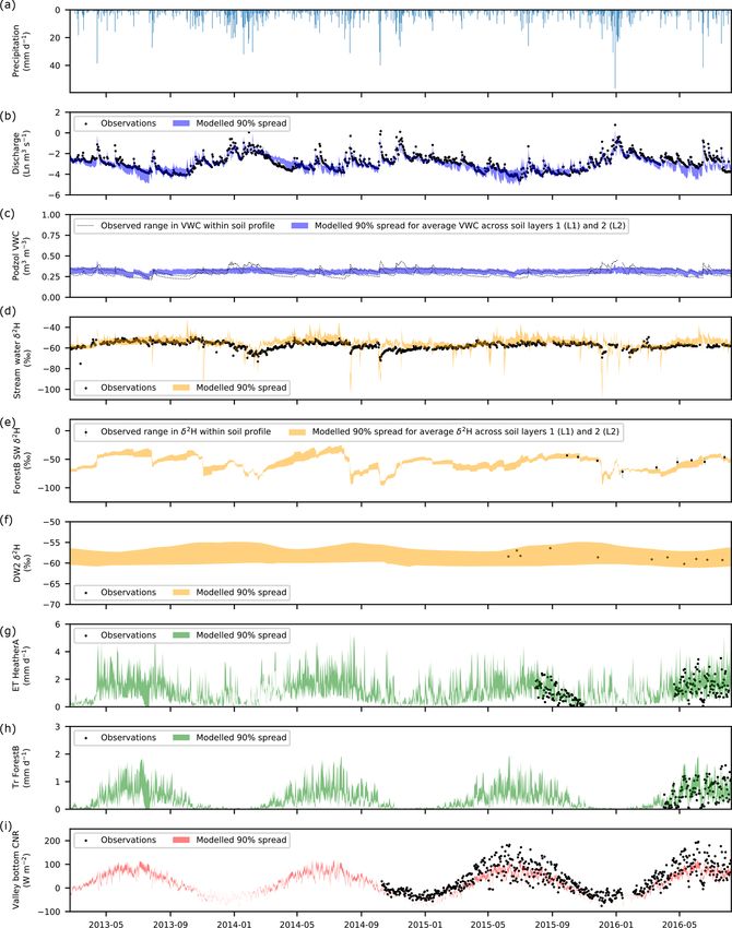
A. J. Neill et al.: Ecohydrological consequences of forest regeneration                                                     4863

tributed models (e.g. Holmes et al., 2020). Consequently, the         Natural Scots pine regeneration is restricted due to graz-
tracer-aided ecohydrological model EcH2 O-iso has recently         ing from high densities of red deer (Cervus elaphus; 11
been developed (Kuppel et al., 2018a). EcH2 O-iso has suc-         to 14.9 deer km−2 ; SNH, 2016) and controlled burning of
cessfully been applied to a range of environments to eluci-        grouse moorlands. Consequently, tree cover is largely lim-
date links between land cover and water partitioning/ages          ited to native pinewoods on the relatively inaccessible steep
(e.g. Douinot et al., 2019; Gillefalk et al., 2021; Knighton       northern hillslope and pine plantations at the catchment
et al., 2020; Kuppel et al., 2020; Smith et al., 2019, 2020).      outlet (Figs. 1 and 2a). Vegetation otherwise reflects soil
    Here, we applied EcH2 O-iso to a small experimental            type; heather (Calluna vulgaris; Erica tetralix) dominates
catchment in the Scottish Highlands to investigate the eco-        the peaty podzols and rankers of the hillslopes, while Molinia
hydrological consequences of natural pinewood regeneration         grassland on the peaty gleys is increasingly outcompeted by
on degraded land. Specifically, we compared a present-day          Sphagnum spp. on the waterlogged peats of the valley bot-
baseline simulation with two land cover change scenarios           tom (Fig. 2a). Isolated pine trees are scattered throughout the
that incorporated forests at early (dense thicket) and late (old   catchment, with those in the wetter valley bottom exhibiting
open forest) stages of regeneration, respectively. Changes         stunted growth (bog pine in Fig. 2a).
to forest structure (proportional vegetation cover, vegetation        Mean annual precipitation is 1000 mm, and potential evap-
heights and leaf area index (LAI) of pine trees) were mod-         otranspiration is 400 mm; the former usually falls in low-
elled for each stage. Soil properties were held constant as        intensity events (< 10 mm d−1 ). Less than 5 % of precipita-
uncertainty surrounds how effective parameters describing          tion is snow, as mean temperatures range between 1 ◦ C in
their aggregated characteristics respond to land cover change      winter and 13 ◦ C in summer. Seepage of fracture flow from
(Seibert and van Meerveld, 2016). Furthermore, the effect of       bedrock outcrops and shallow sub-surface flow through the
conifer forests on soil properties can be unclear, as soil acid-   rankers predominantly move vertically on reaching the pod-
ification from needle decomposition may compete with im-           zols to recharge stores of GW in the underlying drift (Blum-
provements to soil structure caused by increases in organic        stock et al., 2016; Tetzlaff et al., 2014) which sustain base-
matter and root density (Archer et al., 2013; Chappell et al.,     flow conditions in the stream (Blumstock et al., 2015). The
1996). The wet and windy climate of Scotland also makes            storm response of the BB is non-linear, depending on the dy-
it likely that changes in canopy structure and interception        namic expansion of the riparian saturation area which gen-
losses will predominantly determine variations in water par-       erates overland flow and hydrological connectivity between
titioning (see Farley et al., 2005; Marc and Robinson, 2007).      the hillslopes and valley bottom (Birkel et al., 2015; Soulsby
Our specific objectives were to evaluate the effect of forest      et al., 2015).
structure at different stages of regeneration on the following:
    1. dynamics of water flux partitioning in time and space,
                                                                   3     Methods
    2. ages of blue and green water fluxes, and
                                                                   3.1    The EcH2 O-iso model
    3. hydrological connectivity under contrasting flow condi-
       tions.
                                                                   EcH2 O-iso is a development of the ecohydrological model
                                                                   EcH2 O (Maneta and Silverman, 2013). It consists of three
2    Study site                                                    tightly coupled modules simulating the water balance, verti-
                                                                   cal energy balance and vegetation growth dynamics and an
The Bruntland Burn (BB) catchment (3.2 km2 ) is in the             additional fourth module that tracks the stable water isotope
Cairngorms National Park in the Scottish Highlands (Fig. 1).       composition and ages of hydrological stores and fluxes (Kup-
It is a tributary of the Girnock Burn catchment (31 km2 ) that     pel et al., 2018a). The model domain is defined by a regularly
drains into the River Dee. The River Dee supports a glob-          gridded digital elevation model (DEM) that sets local flow
ally important Atlantic salmon (Salmo salar) population and        directions, and governing equations are solved for fixed time
provides drinking water to over 300 000 people (Langan et          steps using finite differences. Proportional coverages of dif-
al., 1997; Soulsby et al., 2016). The glacial legacy of the        ferent vegetation types (based on physiology and structure)
catchment has left steep hillslopes and a flat valley bottom.      and bare soil are specified for each grid cell.
Bedrock is mostly granite with schists and other metamor-             The energy balance is resolved sequentially for the canopy
phic rocks fringing the catchment. This is overlain by exten-      and soil surface. For the canopy, latent (due to transpira-
sive drift deposits (70 % of catchment area) that are 5–10 m       tion and evaporation of intercepted water) and sensible heat
deep on the lower hillslopes and up to 40 m deep in the val-       fluxes depend on canopy temperature; this is determined iter-
ley bottom (Soulsby et al., 2016). Peat (up to 4 m deep) and       atively, such that latent and sensible heat fluxes balance with
peaty gley soils overlay the deeper drift deposits, with peaty     available net radiation. Interception evaporation is limited by
podzols and poorly developed rankers characterising higher         available intercepted water, while a Jarvis-type stomatal con-
elevations along with some bedrock outcrops (Fig. 1a).             ductance model limits transpiration. Transpiration demand is

https://doi.org/10.5194/hess-25-4861-2021                                       Hydrol. Earth Syst. Sci., 25, 4861–4886, 2021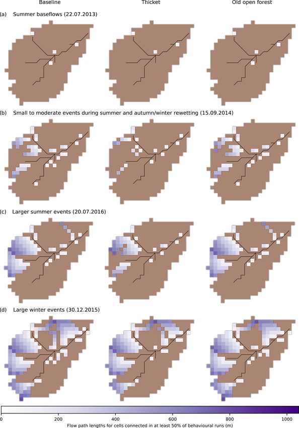
4864                                                      A. J. Neill et al.: Ecohydrological consequences of forest regeneration

Figure 1. Characteristics of the Bruntland Burn catchment. (a) Map showing the distribution of soil types, monitoring sites (DW is deeper
groundwater well) and elevation contours. (b) Aerial view showing the current distribution of vegetation types in the catchment; yellow and
red boxes show areas of established natural forest and land managed for plantations, respectively, while the direction of the photo is shown
by the arrow in panel (a). (c) Map of regeneration potential (partial pinewood regeneration signifies areas where regeneration was limited to
due to presence of scree/exposed bedrock). Photograph in panel (b) by Aaron J. Neill.

satisfied by root water uptake from three soil layers (L1–               model boundary, move laterally as GW simulated via a kine-
3, with L1 being the topmost layer), each with a calibrated              matic wave model or seep into the stream channel. The kine-
depth. Uptake from each layer is proportional to its water               matic wave model assumes that L3 is parallel to the surface,
content and fraction of roots it contains. The latter is deter-          and therefore, flow velocity is proportional to terrain slope
mined by an exponential function describing how the root                 and the horizontal effective hydraulic conductivity. The lat-
fraction decreases with depth (Kuppel et al., 2018b). At the             ter, along with an exponential function describing how resis-
soil surface, iteratively determined temperature partitions net          tance to flow across the channel–subsurface boundary varies
radiation and heat advected by rainfall/throughfall into la-             with gravitational water depth, also controls the rate at which
tent heat for snowmelt and soil evaporation from L1, sensi-              seepage to the stream occurs. Water remaining in ponded
ble heat exchanges between the soil and atmosphere, and heat             storage is routed to the next downslope cell as overland flow
into the ground and snowpack. Soil evaporation is limited by             that can potentially reach the stream within one time step if
the moisture content of L1. In addition to soil, two further             it is not reinfiltrated along the way. Channel routing is simu-
hydrological stores are conceptualised, namely canopy in-                lated using a kinematic wave model. Isotopes and water ages
terception storage and ponded water. Once interception stor-             are tracked assuming complete mixing (Eq. 1 in Smith et al.,
age is full, throughfall reaches the ponded water store where            2020), with fractionation due to evaporation in L1 simulated
it may infiltrate into L1 based on the Green–Ampt model                  via the Craig–Gordon model (Craig and Gordon, 1965; Kup-
(Mein and Larson, 1973). Vertical redistribution of water oc-            pel et al., 2018a). Vegetation growth dynamics were not sim-
curs via gravitational drainage when volumetric water con-               ulated in this application; consequently, vegetation charac-
tent in any of the soil layers exceeds field capacity. Drainage          teristics were static for each scenario. For further details of
rates are proportional to the water content in the layer until           EcH2 O and EcH2 O-iso, see Kuppel et al. (2018a, b), Maneta
they reach effective vertical saturated hydraulic conductiv-             and Silverman (2013) and Smith et al. (2020).
ity. Gravitational water in L3 can leak through the bottom

Hydrol. Earth Syst. Sci., 25, 4861–4886, 2021                                              https://doi.org/10.5194/hess-25-4861-2021

A. J. Neill et al.: Ecohydrological consequences of forest regeneration                                                                 4865

Figure 2. Maps showing the (a) proportional vegetation coverage in the present-day baseline scenario and changes in vegetation cover for
the (b) thicket scenario and (c) old open forest scenario. Changes are reported as the regeneration scenario minus baseline scenario. In panel
(a), coverages of zero are signified by brown cells.

3.2   Present-day baseline scenario                                      less surface, respectively. All vegetation heights in the base-
                                                                         line scenario were based on local knowledge (Table 1).
Catchment soil distribution was based on major Hydrology
of Soil Types (HOST) classifications (Fig. 1a; Tetzlaff et               3.3    Baseline calibration
al., 2007). The properties of each individual soil type were
assumed to be spatially uniform. In total, five vegetation               The baseline scenario was simulated from 21 February 2013
types characterised the present-day baseline scenario, i.e.              to 8 August 2016 on a 100 m × 100 m grid with a daily time
pre-existing Scots pine, heather (also used to represent other           step. Model forcing data are detailed in the Supplement (Ta-
understorey shrubs such as bilberry), Molinia grass, Sphag-              ble S1). A total of 6 years of looped data were used to spin-
num and bog pine (Table 1). Lidar-based estimates of canopy              up the model for calibration, while 30 years were used for
cover were used to derive proportional tree coverages in each            post-calibration runs to stabilise water ages (see Kuppel et
cell (see Kuppel et al., 2018b). Trees on the podzols/rankers            al., 2020). Calibration followed a Morris sensitivity anal-
(plus those in plantations) and on the wetter peat/peaty gleys           ysis (Morris, 1991; Sohier et al., 2014) to identify sensi-
were designated as pre-existing pine and bog pine, respec-               tive parameters (Table S2). For efficiency, it was assumed
tively (Fig. 2a). This permitted explicit representation of              that pre-existing pine and bog pine vegetation types could
stunted growth in the latter due to waterlogging (McHaffie et            take the same parameter values, except for LAI (italics sig-
al., 2002). The extents of remaining vegetation types (Table             nify model parameter names); thus, only four sets of vege-
1; Fig. 2a) were derived from the soil distribution, field map-          tation parameters required calibration. Overall, 90 parame-
ping and aerial imagery (Kuppel et al., 2018b; Tetzlaff et al.,          ters (10 × 4 for soil, 12 × 4 for vegetation and 2 for stream
2007). To account for scree and exposed bedrock (Fig. 1a),               channel) were calibrated. The parameter space was sampled
some rankers on the western and northern hillslopes were set             by conducting 100 000 Monte Carlo simulations. Parameter
with bare earth coverages of 80 % and up to 95 % of the tree-            values were drawn from initial ranges informed by Kuppel

https://doi.org/10.5194/hess-25-4861-2021                                               Hydrol. Earth Syst. Sci., 25, 4861–4886, 2021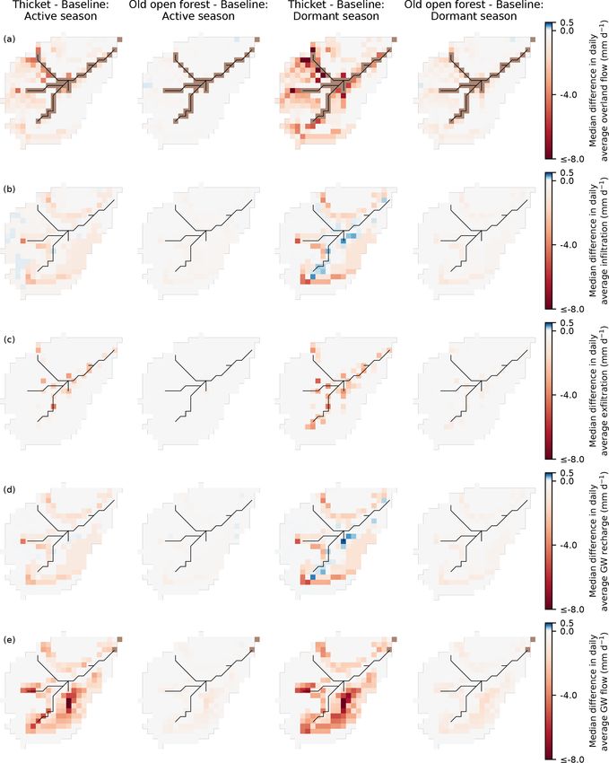
4866                                                                     A. J. Neill et al.: Ecohydrological consequences of forest regeneration

Table 1. Vegetation types in each scenario organised by soil type. All vegetation types are shown for the baseline scenario while only those
in areas of pinewood regeneration on podzols/rankers or wooded bog on peaty gleys are given for the regeneration scenarios (see Fig. 1c).
In areas where regeneration is not possible, vegetation characteristics remain as they were in the baseline scenario. The total coverage of all
vegetation types plus bare earth sum to 100 % within each cell of a given soil type. Leaf area index (LAI) scale factors convert calibrated
values of LAI for pre-existing pine to LAI values for thicket, old open or bog pine.

       Scenario and soil type          Vegetation type            Proportional aerial coverage                                     Height (m)         LAI scale factor
       Baseline
       Podzol and ranker               Pre-existing pine          Lidar derived                                                               10                        1
                                       Heather                    95 % of treeless area, except in existing na-                              0.4                        –
                                                                  tive pinewoods (40 % of treeless area to account
                                                                  for rocky terrain), plantations (0 %) or areas of
                                                                  scree/bedrock (5 % to 20 % of treeless area)
                                       Molinia grass              99 % of treeless area in plantations                                       0.5                        –
       Peaty gley                      Pre-existing pine          Lidar derived in plantations                                                10                        1
                                       Bog pine                   Lidar derived                                                              3.4                    0.17
                                       Heather                    5 % of treeless area, except in plantations (0 %)                          0.4                        –
                                       Molinia grass              99 % of treeless and shrubless area                                        0.5                        –
       Peat                            Pre-existing pine          Lidar derived in plantations                                                10                        1
                                       Bog pine                   Lidar derived                                                              3.4                    0.17
                                       Sphagnum                   70 % of treeless area, except in the northwest                             0.1                        –
                                                                  (90 % of treeless area)
                                       Molinia grass              99 % of treeless and mossless area                                         0.5                        –
       Thicket forest
       Podzol and ranker               Thicket pine               95 % of available pinewood regeneration areaa                           12.7b                     1.37
                                       Heather                    9 % of available treeless pinewood regeneration                         0.12c                         –
                                                                  areac
       Peaty gley                      Bog pine                   15 % of available wooded bog aread                                         2.4                    0.04
                                       Heather                    75 % of available treeless wooded bog areae                                0.4                        –
                                       Molinia grass              99 % of available treeless and shrubless wooded                            0.5                         -
                                                                  bog areae
       Old open forest
       Podzol and ranker               Old open pine              54 % of available pinewood regeneration areaa                           15.5b                     0.59
                                       Heather                    82 % of available treeless pinewood regenera-                           0.29c                         –
                                                                  tion areac
       Peaty gley                      Bog pine                   15 % of available wooded bog aread                                         8.4                      0.4
                                       Heather                    75 % of available treeless wooded bog areae                                0.4                        –
                                       Molinia grass              99 % of available treeless and shrubless wooded                            0.5                        –
                                                                  bog areae

     Note: a Based on plan drawings of thicket (type 25) and old open forest (type 3) as seen in Fig. 3 of Summers et al. (1997). b Median height of aged trees from thicket
     and old open woodland as seen in Table 2 of Summers et al. (2008). c Sum of shrub cover or cover-weighted average height of shrubs for thicket and old open pines in
     Table 1 of Parlane et al. (2006). d Based on pine cover in uncut wooded bogs reported by McHaffie et al. (2002). e Based on field descriptions of Steven and
     Carlisle (1959).

Hydrol. Earth Syst. Sci., 25, 4861–4886, 2021                                                                      https://doi.org/10.5194/hess-25-4861-2021
A. J. Neill et al.: Ecohydrological consequences of forest regeneration                                                     4867

et al. (2018b) and additional literature reviews (Table S2).       3.4   Regeneration scenarios
The LAI of bog pine was related to the sampled LAI of pre-
existing pine via a scale factor accounting for relative differ-   Extensive work characterising the structure of native pine
ences in canopy architecture. The scale factor (0.17) was de-      stands at Abernethy Forest in the Cairngorms National Park
rived by dividing an empirical estimate of LAI for bog pine        (Parlane et al., 2006; Summers, 2018; Summers et al., 1997,
by a local measurement of LAI for pre-existing Scots pine          2008) was used to select two stages of forest regeneration
(Wang et al., 2018). The former was obtained by first estimat-     for simulation. For context, Fig. S1 in the Supplement sum-
ing the fraction of above-canopy irradiance passing through        marises the general sequence of natural pinewood regener-
the canopy as a function of tree height (3.4 m) and density        ation. The thicket stage has the highest tree densities and
(275 trees ha−1 ; Summers et al., 1997) via the equation of        near-complete canopy closure; consequently, this stage was
Parlane et al. (2006). This was then used in Beer’s law with       selected because it will likely have the most substantial im-
a light extinction coefficient of 0.5 (White et al., 2000) to      pact on water partitioning and catchment hydrology. Trees
determine LAI.                                                     are ∼ 40 years old, while understorey development is lim-
   Diverse ecohydrological and isotope data sets were avail-       ited. Old open forest was chosen as the second stage and rep-
able at the BB catchment for model calibration (Table 2).          resents a possible realisation of old-growth forest. This stage
Protocols used to collect and process these data are detailed      may be somewhat semi-natural, with a canopy that is per-
in Kuppel et al. (2018a, b). In most cases, model outputs were     haps too open as a consequence of past silvicultural practices
directly compared against relevant observed data sets. Simu-       and upland grazing (Summers et al., 2008). Consequently,
lated soil variables (volumetric water content and bulk water      regeneration of such a forest would require a rewilding tra-
isotopes) were exceptions; these are output for each soil layer    jectory that seeks to restore natural regeneration while also
and, therefore, do not directly correspond to depth-specific       employing passive management to preserve characteristics
observations (see Beven, 2006). To accommodate this, sim-          of a landscape that reflects elements of Scottish cultural her-
ulated volumetric water content time series for L1 and L2          itage and/or the habitats provided by such a semi-natural en-
were compared to observations made at the depth closest to         vironment (see Deary and Warren, 2017). Nonetheless, it was
the mid-point of each layer. Meanwhile, simulated soil wa-         chosen as a possible lowest impact stage of late forest devel-
ter isotopes in L1 and L2 were compared with the average           opment and, thus, offers an extreme contrast to the thicket
of observations made within the soil profile encompassed by        scenario. Trees are tall, old (∼ 150 years) and sparsely dis-
each respective layer. Consequently, observations compared         tributed, with an understorey of well-developed shrubs.
to simulated outputs from L1 and L2 could vary, depending             The proportional coverage and characteristics of vegeta-
on soil depth parameterisation.                                    tion at each stage of forest regeneration are given in Ta-
   Model skill in simulating the dynamics of ecohydrologi-         ble 1. Native pinewoods, consisting of thicket/old open pine
cal and isotopic observations was quantified using the perfor-     and a heather understorey, were assumed to fully regener-
mance metrics in Table 2. Mean absolute error was used for         ate on podzols and rankers (Fig. 1c), reflecting the prefer-
discharge to avoid over-emphasis of high flows that can occur      ence of pine for freely draining minerogenic soils (Mason
when using metrics based on mean squared errors (Krause            et al., 2004). The available regeneration area was limited in
et al., 2005). It was further used for all isotope simulations     ranker cells containing scree or exposed bedrock such that
given the limited variability in observations and the daily        the bare earth fraction remained constant across scenarios,
time step of the model (see Gupta et al., 2009; Schaefli and       while regeneration did not occur on managed land at the
Gupta, 2007). Root mean squared error was otherwise used           catchment outlet or in pre-existing areas of native pinewood
as this is recommended if no information is available on error     on the northern hillslope (Fig. 1c). A wooded bog consisting
distributions (Chai and Draxler, 2004; Kuppel et al., 2018b).      of stunted bog pine, heather and Molinia grass, was simu-
To determine behavioural parameter sets, model runs were           lated on the wetter peaty gleys (McHaffie et al., 2002; Steven
first selected that simulated saturation areas < 60 % of total     and Carlisle, 1959; Summers et al., 1997), while no regener-
catchment area for at least 90 % of the simulation period; this    ation was possible on the waterlogged peat (Fig. 1c). Spatial
reflected mapping and modelling of the extent of saturation        changes in vegetation cover for each regeneration scenario
in the BB catchment (Birkel et al., 2010). Performance met-        relative to the baseline are shown in Fig. 2b–c. Scale fac-
rics for each calibration data set were then ranked across all     tors relating calibrated values of LAI for pre-existing pine
runs that satisfied this constraint. Runs were finally ordered     to the LAI of thicket, old open and bog pine were calcu-
by their worst-performing metric, with the best 30 runs be-        lated as described in Sect. 3.3. For thicket/old open pine,
ing retained as behavioural; this balanced the need to illus-      measured fractions of the above-canopy irradiance passing
trate uncertainty in model outputs with the increased compu-       through the canopy were available from Parlane et al. (2006).
tational demand of producing spatial outputs required post-        Estimates for bog pine were again made via the equation of
calibration.                                                       Parlane et al. (2006). The heights of bog pine in each sce-
                                                                   nario were estimated by first calculating a stunted growth
                                                                   rate (∼ 0.06 m yr−1 ) by dividing the height of present-day

https://doi.org/10.5194/hess-25-4861-2021                                       Hydrol. Earth Syst. Sci., 25, 4861–4886, 2021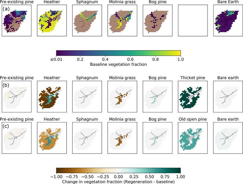
4868                                                                    A. J. Neill et al.: Ecohydrological consequences of forest regeneration

Table 2. Data sets used in the calibration of EcH2 O-iso and their temporal coverage (full study period is 21 February 2013 to 8 August 2016).
Performance metrics used to quantify the skill of the model in simulating each data set and the range of values achieved by the 30 behavioural
model runs are also given.

         Data set                                          Temporal coverage                                      Metric a       Behavioural range
         Streamflow                                        Full study period                                      MAE            0.026 to 0.033 m3 s−1
         Soil moisture content
         Forest A (10, 20 and 40 cm)                       Full study period                                      RMSE           b 0.10 to 0.27 m3 m−3

         Forest B (10, 20 and 40 cm)                       25 February 2015 onwards                               RMSE           b 0.11 to 0.19 m3 m−3

         Gley (10, 30 and 50 cm)                           Full study period                                      RMSE           b 0.04 to 0.29 m3 m−3

         Heather A (10, 20 and 40 cm)                      Full study period                                      RMSE           b 0.06 to 0.27 m3 m−3

         Peat (10 cm)                                      Full study period                                      RMSE           0.02 to 0.10 m3 m−3
         Peaty podzol (10, 30 and 50 cm)                   Full study period                                      RMSE           b 0.03 to 0.11 m3 m−3

         Green fluxes
         Heather A – transpiration and                     31 July to 30 October 2015 and                         RMSE           c Tr – 0.50 to 0.69 mm d−1 ;
         evapotranspiration                                21 April to 3 August 2016                                             ET – 0.81 to 1.16 mm d−1
         Heather B – transpiration and                     31 July to 30 October 2015 and                         RMSE           c Tr – 0.43 to 0.60 mm d−1 ;
         evapotranspiration                                31 March to 11 July 2016                                              ET – 0.78 to 0.95 mm d−1
         Forest A – transpiration                          8 July to 27 September 2015                            RMSE           0.33 to 0.70 mm d−1
         Forest B – transpiration                          1 April 2016 onwards                                   RMSE           0.22 to 0.39 mm d−1
         Net radiation
         Bog weather station                               10 October 2014 to 3 August 2016                       RMSE           29 to 36 W m−2
         Hilltop weather station                           22 April 2015 onwards                                  RMSE           40 to 58 W m−2
         Valley bottom weather station                     10 October 2014 onwards                                RMSE           29 to 39 W m−2
         Streamflow – δ 2 H                                Full study period                                      MAE            2.7 ‰ to 8.2 ‰
         Soil δ 2 H (2.5, 7.5, 12.5 and
         17.5 cm)
         Forest A – bulk soil water                        29 September 2015 onwards (monthly)                    MAE            b 3.4 ‰ to 20.6 ‰

         Forest B – bulk soil water                        29 September 2015 onwards (monthly)                    MAE            b 3.8 ‰ to 7.5 ‰

         Heather A – bulk soil water                       29 September 2015 onwards (monthly)                    MAE            b 2.6 ‰ to 21.5 ‰

         Heather B – bulk soil water                       29 September 2015 onwards (monthly)                    MAE            b 4.2 ‰ to 8.2 ‰

         Groundwater δ 2 H
         Deeper well 1 (peat)                              11 samples between 9 June 2015 and                     MAE            0.4 ‰ to 5.4 ‰
                                                           22 July 2016
         Deeper well 2 (peat)                              11 samples between 9 June 2015 and                     MAE            0.7 ‰ to 2.9 ‰
                                                           22 July 2016
         Deeper well 3 (peaty gley)                        11 samples between 9 June 2015 and                     MAE            0.7 ‰ to 6.7 ‰
                                                           22 July 2016
         Deeper well 4 (peaty podzol)                      11 samples between 9 June 2015 and                     MAE            0.7 ‰ to 3.4 ‰
                                                           22 July 2016

       Note: a MAE is the mean absolute error, and RMSE is the root mean squared error. b Range across first two soil layers of EcH2 O-iso. c Tr is transpiration, and
       ET is evapotranspiration.

Hydrol. Earth Syst. Sci., 25, 4861–4886, 2021                                                                    https://doi.org/10.5194/hess-25-4861-2021
A. J. Neill et al.: Ecohydrological consequences of forest regeneration 4869
bog pine by an assumed age of 60 years. This was multi- To assess how regeneration impacts hydrological source
plied by the age of pines in the thicket (40 years) and old areas and runoff generation, the spatial extent of hydro-
open (150 years) forests to give bog pine heights of 2.4 logical connectivity was quantified under contrasting flow
and 8.4 m for each scenario, respectively. These values are conditions. A cell was considered hydrologically connected
broadly consistent with height measurements made by Sum- if overland flow (OLF) was simulated for the cell and all
mers et al. (2008) on bog pine trees with an interquartile age downslope cells along the flow path to the stream. No min-
range between 72 and 143 years. imum threshold of OLF was imposed for a cell to be con-
Simulations were driven by the 30 behavioural parame- sidered connected (see Turnbull and Wainwright, 2019),
ter sets obtained from the baseline calibration and under- as EcH2 O-iso simulates re-infiltration along a given flow
taken for the same time period (21 February 2013 to 8 Au- path which can prevent upslope cells producing OLF from
gust 2016) with 30 years of spin-up. As previously stated, connecting to the stream (Maneta and Silverman, 2013).
soil properties remained unchanged in the regeneration sce- Flow path lengths for connected cells were calculated by
narios. Additionally, the vertical root distribution param- accumulating the straight line or diagonal lengths (depen-
eter was consistent amongst pine vegetation types as af- dent on local flow direction) of all cells along the flow
ter the sapling stage; the most significant changes to Scots path (see Turnbull and Wainwright, 2019). A total of four
pine rooting characteristics are expressed in the horizontal different flow conditions were considered for the connec-
rather than vertical direction (Laitakari, 1927; Makkonen and tivity analysis, with each assessed using OLF simulations
Helmisaari, 2001). Potential effects of such changes on the from a representative date, as follows: (1) summer baseflows
vertical root distribution would likely already be captured by (22 July 2013), (2) small to moderate events during summer
the sampling range of this parameter for pre-existing pine and autumn/winter rewetting (15 September 2014), (3) larger
(Table S2). summer events (20 July 2016) and (4) large winter events
(30 December 2015).
3.5 Change analysis
To contextualise changes to water flux partitioning, simu- 4 Results
lated maximum root zone and interception storage capacities
were quantified for each scenario. For each vegetation type 4.1 Baseline calibration
in a given grid cell, root zone storage capacity was defined as
the sum of maximum plant-available volumetric water con- Figure 3 summarises the skill of the model in simulating blue
tent in each layer weighted by root fraction, multiplied by the and green fluxes, isotope dynamics and net radiation at se-
coverage-weighted average rooting depth of all vegetation lected monitoring locations (remaining simulations shown in
types in the cell. A coverage-weighted sum across all present Figs. S2–S5). Performance metrics and calibrated parameter
vegetation types then yielded the total root zone storage ca- ranges are given in Tables 2 and S2, respectively. Stream dis-
pacity for the cell. The total interception storage capacity of charge was generally well simulated, with only occasional
each cell was similarly calculated, with the interception stor- under-prediction of baseflows (e.g. summer 2016) and the
age capacity of each vegetation type obtained by multiplying most extreme events. At most sites, modelled volumetric wa-
the parameters LAI and maximum canopy storage (Table S2). ter content in L1 and L2 was bracketed by the range observed
Values of root zone and interception storage capacity at the across the soil profile, although simulations were sometimes
catchment scale were then derived. less dynamic than observations, and root mean squared errors
Catchment-scale flux partitioning was assessed by quanti- could be large. However, this likely reflects the commensu-
fying seasonally averaged flux totals for simulated discharge rability issues highlighted in Sect. 3.3 (also relevant for soil
at the outlet, GW recharge, soil and interception evaporation, water isotopes), and the fact that Heather A and Forest A fell
and transpiration. Seasons were defined as April to Septem- within the same model cell. The model was generally suc-
ber (active season) and October to March (dormant season), cessful in reproducing dynamics of stream water, soil water
broadly corresponding to biologically active and dormant pe- and groundwater isotopes, implying internal catchment func-
riods in northeastern Scotland, respectively (Dawson et al., tioning was reasonably well captured. Stream isotopes were
2008). Seasonal volume-weighted average water ages were sometimes over-enriched, suggesting slightly high soil evap-
also calculated for selected stores and fluxes. Daily time se- oration; however, the variability was generally well captured.
ries of discharge, stream isotopic composition and water age Larger deviations during events likely reflect structural lim-
provided a spatially integrated insight into how regeneration itations of the model (e.g. the ability of OLF to traverse the
affected modelled catchment hydrology at a higher tempo- catchment within one time step). Excessive evaporation was
ral resolution. To better understand spatial drivers of changes not apparent from simulated soil water isotopes, although av-
to catchment-scale flux partitioning, differences in seasonal eraging over L1 and L2 could obscure the effects of evapora-
daily average blue and green fluxes between each scenario tive fractionation in the former. The model had skill in sim-
and the baseline were spatially disaggregated. ulating ET and forest transpiration. However, underestima-
https://doi.org/10.5194/hess-25-4861-2021 Hydrol. Earth Syst. Sci., 25, 4861–4886, 20214870 A. J. Neill et al.: Ecohydrological consequences of forest regeneration
tion of heather transpiration may indicate excessive radiative between the old open forest and baseline, resulting in the me-
energy being used for evaporation. Seasonality in net radia- dian and 5th and 95th percentile seasonally averaged flux to-
tion was well simulated, though shorter-term variability was tals generally being similar for the two scenarios. However,
under-estimated in summer. there was a repartitioning of water between increased inter-
ception evaporation and reduced GW recharge for the dor-
4.2 Impact of regeneration on water storage capacity mant season that contributed to an ∼ 30 mm decrease in the
median seasonally averaged discharge total.
Figure 4 summarises simulated root zone and intercep-
tion storage capacities for each scenario. Median root zone 4.4 Spatiotemporal dynamics of baseline flux
storage capacity increased by 21 mm in the thicket forest partitioning
scenario, reflecting replacement of heather by thicket pine
(Fig. 2b) with deeper roots (Table S2) that increase access to Figure 6 summarises the spatial dynamics of median seasonal
water stored in L2 and L3. Small increases in root zone stor- daily average blue and green fluxes for the baseline scenario.
age capacity were simulated for the old open forest scenario, Simulated OLF was more limited for the active season. The
albeit with greater overlap with the baseline, likely reflect- largest fluxes were simulated for the peats and peaty gleys,
ing the more balanced composition between pine and heather with some OLF also being generated by the ranker soils on
(Fig. 2c). This, along with greater proportional coverage of the hillslopes. The latter is interpreted as representing the
bare earth (Fig. 2c), may also explain overlap of interception rapid near-surface flows in the shallow rankers that are driven
storage capacity between the old open forest and baseline by the emergence of bedrock fracture flow at slope breaks.
scenarios. The greater coverage of thicket pine (Fig. 2b) with OLF fluxes were greater and had similar spatial patterns for
a dense canopy substantially increased interception storage the dormant season, with additional fluxes generated from
capacity for the thicket forest scenario. the podzols on lower hillslopes in the north and south. Ver-
tical movement of water (infiltration and GW recharge) was
4.3 Changes to catchment-scale water flux partitioning greatest in the dormant season and mostly occurred on the
podzols; the largest fluxes were simulated at the boundaries
Figure 5 shows how impacts of modelled regeneration in- between the podzols and rankers reflecting lateral flows from
tegrated to affect the simulated quantity and isotopic com- upslope moving vertically in deeper soils. Water was then
position of streamflow. Discharge was most notably reduced simulated to move downslope as GW to sustain saturation
in the thicket scenario. Proportional reductions in discharge in the valley bottom, as evidenced by high exfiltration fluxes
(as revealed by considering its natural logarithm) appeared especially in the dormant season.
to show an annual cycle, generally increasing in magni- Daily average fluxes of ET were simulated as being great-
tude through the summer months and into the autumn/winter est for the active season, particularly in the valley bottom
rewetting period before being reset by a sufficiently large (Fig. 6). This was facilitated by the wet peat and peaty gleys
winter event that resulted in more limited divergence of sub- maintaining transpiration and soil evaporation and by evapo-
sequent winter and spring flows. Consequently, low to mod- ration of water intercepted by the Sphagnum canopy. Domi-
erate flows during the summer and autumn/winter rewet- nance of vertical sub-surface fluxes limited transpiration and,
ting period were most affected in the thicket scenario, while particularly, soil evaporation from the podzols, reducing to-
higher flows remained relatively consistent. For the old open tal ET fluxes. For the dormant season, spatial patterns in total
forest scenario, discharge was similar to the baseline. For ET were less distinct, reflecting reduced soil and interception
both regeneration scenarios, simulated stream isotope dy- evaporation in the valley bottom and the fact that daily tran-
namics were comparable to the baseline; however, stream spiration fluxes were essentially zero. A notable pattern was
water could sometimes be slightly more depleted in summer that total ET was particularly elevated where there was sub-
for the thicket scenario, indicating reduced soil evaporation. stantial pre-existing pine (Figs. 2a and 6f) due to sustained
Table 3 summarises the changes to seasonally averaged interception evaporation.
water flux totals. Overall, behavioural models consistently
simulated a decrease in seasonally averaged discharge for the 4.5 Spatiotemporal disaggregation of regeneration
thicket scenario. This resulted from increased interception effects on flux partitioning
evaporation and transpiration and decreased GW recharge.
Recharge was most reduced for the dormant season, con- Median differences in seasonal daily average blue fluxes
current with the greatest increase in interception evapora- were most dramatic for the thicket scenario (Fig. 7). For
tion. Soil evaporation was lower for the thicket scenario, both the active and dormant seasons, similar spatial patterns
likely reflecting limits imposed by lower soil moisture due to were simulated, although differences tended to be greater for
greater interception evaporation and transpiration losses, and the latter. More limited OLF generation by the rankers led
reduced penetration of radiation through the thicket canopy. to similar magnitude reductions in daily average infiltration
Differences in seasonally averaged fluxes were much smaller and GW recharge on the podzols. Consequently, downslope
Hydrol. Earth Syst. Sci., 25, 4861–4886, 2021 https://doi.org/10.5194/hess-25-4861-2021A. J. Neill et al.: Ecohydrological consequences of forest regeneration 4871 Figure 3. Time series of (a) precipitation and of the observed and simulated (b) natural logarithm (Ln) of stream discharge. (c) Volumetric water content (VWC) at the peaty podzol site. (d) Stream δ 2 H composition. (e) Bulk soil water (SW) δ 2 H under Forest B. (f) Groundwater δ 2 H at deeper well 2 (DW2). (g) Total evapotranspiration (ET) for Heather A. (h) Transpiration (Tr) for Forest B. (i) Net radiation (CNR) at the valley bottom weather station. The 90 % spread of simulations are from the 30 behavioural model runs. https://doi.org/10.5194/hess-25-4861-2021 Hydrol. Earth Syst. Sci., 25, 4861–4886, 2021
4872                                                      A. J. Neill et al.: Ecohydrological consequences of forest regeneration

Table 3. Seasonally averaged water flux totals and differences in seasonally averaged totals. Totals and differences were calculated for each
behavioural run individually and summarised by the median and 5th and 95th percentile (in parentheses) values across all behavioural runs.
Differences are reported as the regeneration scenario minus baseline and help to indicate whether the simulated direction of change in each
flux was consistent among behavioural models. Active and dormant seasons cover April to September and October to March, respectively.

                                      Median (5th and 95th percentile) seasonally    Median (5th and 95th percentile) differences
                                            averaged flux totals (mm over                in seasonally averaged flux totals
                                                  summary period)                           (mm over summary period)
                                              Active                     Dormant               Active                    Dormant
          Outlet stream discharge
          Baseline                    196 (159, 232)               449 (415, 481)                –                            –
          Thicket                      143 (97, 202)               316 (258, 435)    −64 (−97, −8)             −129 (−178, −26)
          Old open forest             190 (159, 230)               416 (369, 486)    −12 (−31, 18)                −29 (−59, 15)
          Groundwater recharge
          Baseline                    161 (140, 190)               353 (283, 402)                –                            –
          Thicket                      107 (68, 156)               277 (224, 349)    −63 (−93, −5)              −80 (−109, −15)
          Old open forest             153 (129, 185)               336 (269, 382)     −9 (−27, 19)                 −18 (−37, 6)
          Interception evaporation
          Baseline                     102 (81, 131)                  77 (62, 90)                  –                             –
          Thicket                     182 (104, 234)               196 (102, 253)       83 (−3, 124)                 118 (27, 168)
          Old open forest              116 (74, 159)                106 (61, 150)       19 (−24, 43)                 31 (−10, 64)
          Soil evaporation
          Baseline                       74 (52, 94)                   41 (35, 45)               –                             –
          Thicket                        44 (34, 57)                   28 (22, 34)   −32 (−47, −8)                 −12 (−17, −7)
          Old open forest                72 (55, 91)                   37 (32, 41)    −2 (−12, 13)                    −4 (−6, 0)
          Transpiration
          Baseline                       66 (52, 80)                      6 (4, 8)                  –                             –
          Thicket                       89 (71, 121)                    12 (9, 20)        27 (11, 47)                     6 (3, 13)
          Old open forest                58 (45, 76)                      6 (5, 8)       −7 (−14, 3)                     0 (−1, 2)

movement of GW also decreased in both seasons. This con-                    Differences in seasonal daily average green fluxes were
tributed to a drying out of the valley bottom (especially in the         also more apparent in the thicket scenario (Fig. 8). Daily
dormant season), even though local regeneration was lim-                 average ET from the podzols and rankers was simulated
ited (Fig. 2b). Daily average OLF fluxes were simulated to               to increase throughout the year. For the active season, this
decrease around the fringes of the stream for both seasons.              resulted from greater transpiration and, predominantly, in-
The largest decreases occurred in the northwest of the catch-            terception evaporation, reflecting the increased coverage of
ment as a direct consequence of reduced OLF from upslope.                thicket pine (Fig. 2b). Reduced penetration of radiative en-
Elsewhere, OLF reductions strongly reflected the reductions              ergy through the thicket canopy, and limits imposed by
in upslope GW subsidies as evidenced by consistently de-                 greater water losses to transpiration and interception evap-
creased exfiltration fluxes and increased infiltration of incom-         oration, decreased simulated daily average soil evaporation.
ing precipitation in the valley bottom for the dormant season            For the dormant season, increased ET was more driven
to replenish drier soil and GW stores.                                   by greater interception evaporation. ET from the wooded
   Similar spatial dynamics were simulated for the old open              bog was similar to the baseline. This was due to decreased
forest scenario; however, median differences in seasonal                 transpiration from reduced cover of potentially deep-rooted
daily average fluxes were much reduced (Fig. 7). It is also              (Aerts et al., 1992; Taylor et al., 2001) Molinia grass (Fig. 2b)
noteworthy that, even in the dormant season, the valley bot-             being compensated by increases in soil and, particularly, in-
tom dried out less than in the thicket scenario; daily average           terception evaporation. Daily average ET for the active sea-
GW flows through the podzols were only simulated to de-                  son decreased in some areas of peat despite no regeneration
crease by < 1.5 mm d−1 , while no increases in infiltration or           having taken place. This would be consistent with drying of
GW recharge were simulated in the valley bottom.                         the valley bottom limiting summer transpiration.

Hydrol. Earth Syst. Sci., 25, 4861–4886, 2021                                              https://doi.org/10.5194/hess-25-4861-2021
A. J. Neill et al.: Ecohydrological consequences of forest regeneration 4873
erate flows, although uncertainty bounds were again wide
(Fig. 5d). Relatively young stream water ages persisted in
larger events. Transpiration fluxes were the only ones to in-
dicate a possible slight preference for younger water through
a reduction in 95th percentile average ages (Table 4). For
old open forest, age characteristics were generally restored
to those simulated for the baseline.
4.7 Changes to hydrological connectivity
For the considered flow conditions, Fig. 9 summarises spa-
tial patterns of hydrological connectivity that were simu-
lated by at least 50 % of the behavioural model runs. Base-
line connectivity during summer baseflows was only estab-
lished for a limited number of cells close to the stream; for
22 July 2013 only ∼ 1 % of cells were connected due to par-
ticularly dry summer conditions at this time (Fig. 9a). In the
thicket scenario, the spatial extent of connectivity became
even more limited, though saturation in the valley bottom
was maintained. Regeneration of old open forest did not sub-
stantially affect connectivity dynamics; indeed, this was the
case for all flow conditions considered. The catchment had a
wetter baseline state for small to moderate summer and au-
tumn/winter rewetting events, with 14 % of cells being con-
nected on 15 September 2014 (Fig. 9b). This reflected greater
Figure 4. Box plots showing maximum (a) root zone storage ca- connectivity in the valley bottom and the establishment of
pacity and (b) interception storage capacity, for the baseline and longer flow paths (up to 600 m) in the west of the catchment.
forest regeneration scenarios. The median is shown by the orange These flow paths tended to become shorter in the thicket
line, while the box extends from the lower to upper quartiles. The scenario; along with slightly less connectivity in the valley
5th and 95th percentiles are given by the tails. bottom, this caused a 52 % reduction in cells that were con-
nected to the stream. Stronger connectivity and longer flow
paths (up to 800 m) in the west of the catchment and estab-
Differences in simulated ET were much more subdued for lishment of a long flow path down the northern hillslope led
the old open forest scenario (Fig. 8). For the active season, to 25 % of cells being connected in the representative larger
soil evaporation on the rankers and podzols, in particular, re- summer event on 20 July 2016 (Fig. 9c). While some cells
mained similar to the baseline, while transpiration showed a with longer flow paths did disconnect in the thicket scenario,
more consistent slight decrease. This offset greater losses to the largest reductions in connectivity resulted from the dis-
interception evaporation so that only small increases in total connection of cells with more moderate flow path lengths (up
ET were simulated. Very small ET decreases mostly reflected to 600 m) in the west of the catchment. Despite this, how-
the replacement of larger clusters of pre-existing pine with ever, large connected areas were maintained in both the west
old open forest (Fig. 2c) leading to reduced transpiration. A of the catchment and valley bottom, leading to a 36 % reduc-
larger increase in interception evaporation from the old open tion in connectivity overall. Large winter events showed the
forest drove the increases in ET from the podzols and rankers greatest baseline connectivity, with 48 % of cells connected
for the dormant season. to the stream on 30 December 2015 (Fig. 9d). This reflected
greater establishment of connectivity on the northern hills-
4.6 Effects of regeneration on ages of blue and green lope and in the southwest headwater that also increased the
water number of connected cells with moderate to long (400 to
1000 m) flow path lengths. Spatial patterns of connectivity
Streamflow, lateral GW outflows and soil water/evaporation were similar overall in the thicket scenario, with the main
were near-consistently simulated to have older average ages notable changes being reduced connectivity in the southwest
in the thicket scenario relative to the baseline (Table 4); how- headwaters and disconnection of specific flow paths on the
ever, change magnitudes were often less than the width of northern hillslopes due to more limited OLF generation from
simulation uncertainty bounds leading to overlap in flux ages. some riparian cells (e.g. around the headwater confluences –
Simulated daily dynamics revealed that stream water ages for Fig. 7a). These changes led to just a 16 % reduction in the
the thicket scenario could be much older for low to mod- total number of cells connected to the stream.
https://doi.org/10.5194/hess-25-4861-2021 Hydrol. Earth Syst. Sci., 25, 4861–4886, 20214874 A. J. Neill et al.: Ecohydrological consequences of forest regeneration
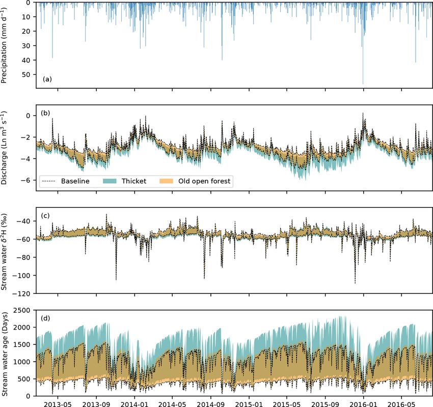
Figure 5. Time series of the (a) observed precipitation and the simulated (b) natural logarithm (Ln) of stream discharge. (c) Stream water
δ 2 H composition. (d) Stream water age. In panels (b) to (d), the area between the two black lines represents the 90 % spread of behavioural
simulations for the baseline scenario, while the shaded areas show the same for the thicket and old open forest scenarios. Areas of darker,
gold-coloured shading occur where simulations for the two regeneration scenarios overlap.
5 Discussion catchment in Scotland by comparing simulated present-day
baseline conditions with two land cover change scenarios
5.1 Simulated effects of natural forest regeneration on representing different stages of forest regeneration (thicket
blue and green water partitioning and old open forest).
The overall skill of the model in capturing the dynam-
Previous studies investigating the hydrological consequences ics of diverse ecohydrological and isotope data sets (Ta-
of changes in forest cover have often sought to understand ble 2; Fig. 3) helped provide confidence in its ability to sim-
how conversion and management of land for commercial ulate plausible realisations of catchment functioning. How-
forestry affects aggregated metrics of catchment hydrologi- ever, despite the rich calibration data set, larger uncertainties
cal functioning (Ellison et al., 2017; Filoso et al., 2017), es- persisted in some model outputs (e.g. water ages; Fig. 5d).
pecially so in the UK context (Marc and Robinson, 2007). This likely reflected a combination of several factors, includ-
Consequently, findings may not be transferable to the case of ing the extent to which available data can constrain specific
passively managed natural forest regeneration that is the goal details of individual processes simulated by complex mod-
of rewilding efforts in degraded landscapes such as the Scot- els alongside more general features of catchment function-
tish Highlands (zu Ermgassen et al., 2018). Therefore, using ing (e.g. surface water vs. GW dominated; Holmes et al.,
the EcH2 O-iso model, we investigated the ecohydrological 2020; Neill et al., 2020), limitations in the information con-
consequences of natural pinewood regeneration for the BB tent of certain data sets (e.g. extent to which isotopes con-
Hydrol. Earth Syst. Sci., 25, 4861–4886, 2021 https://doi.org/10.5194/hess-25-4861-2021You can also read