Stratospheric gravity waves over the mountainous island of South Georgia: testing a high-resolution dynamical model with 3-D satellite ...
←
→
Page content transcription
If your browser does not render page correctly, please read the page content below
Atmos. Chem. Phys., 21, 7695–7722, 2021
https://doi.org/10.5194/acp-21-7695-2021
© Author(s) 2021. This work is distributed under
the Creative Commons Attribution 4.0 License.

Stratospheric gravity waves over the mountainous island of South
Georgia: testing a high-resolution dynamical model with 3-D
satellite observations and radiosondes
Neil P. Hindley1,2 , Corwin J. Wright1 , Alan M. Gadian2 , Lars Hoffmann3 , John K. Hughes2 , David R. Jackson4 , John
C. King5 , Nicholas J. Mitchell1 , Tracy Moffat-Griffin5 , Andrew C. Moss1 , Simon B. Vosper4 , and Andrew N. Ross2
1 Centre for Space, Atmospheric and Oceanic Science, University of Bath, Bath, UK
2 School  of Earth and Environment, University of Leeds, Leeds, UK
3 Jülich Supercomputing Centre, Forschungszentrum Jülich, Jülich, Germany
4 Met Office, Exeter, UK
5 Atmosphere, Ice and Climate Group, British Antarctic Survey, Cambridge, UK

Correspondence: Neil P. Hindley (n.hindley@bath.ac.uk) and Corwin J. Wright (c.wright@bath.ac.uk)

Received: 12 May 2020 – Discussion started: 12 June 2020
Revised: 26 February 2021 – Accepted: 15 March 2021 – Published: 20 May 2021

Abstract. Atmospheric gravity waves (GWs) play an impor-          We find that the timing, magnitude and direction of simulated
tant role in atmospheric dynamics but accurately represent-       GWMF over South Georgia are in good general agreement
ing them in general circulation models (GCMs) is challeng-        with observations, once the AIRS sampling and resolution
ing. This is especially true for orographic GWs generated         are applied to the model. Area-averaged zonal GWMF dur-
by wind flow over small mountainous islands in the South-         ing these 2 months is westward at around 5.3 and 5.6 mPa in
ern Ocean. Currently, these islands lie in the “grey zone” of     AIRS and model sampled as AIRS datasets respectively, but
global model resolution, where they are neither fully resolved    values directly over the island can exceed 50 mPa. However,
nor fully parameterised. It is expected that as GCMs ap-          up to 35 % of the total GWMF in AIRS is actually found
proach the spatial resolution of current high-resolution local-   upwind of the island compared to only 17 % in the model
area models, small-island GW sources may be resolved with-        sampled as AIRS, suggesting that non-orographic GWs ob-
out the need for parameterisations. But how realistic are the     served by AIRS may be underestimated in our model config-
resolved GWs in these high-resolution simulations compared        uration. Meridional GWMF results show a small northward
to observations? Here, we test a high-resolution (1.5 km hor-     bias (∼ 20 %) in the model sampled as AIRS that may cor-
izontal grid, 118 vertical levels) local-area configuration of    respond to a southward wind bias compared to coincident
the Met Office Unified Model over the mountainous island of       radiosonde measurements. Finally, we present one example
South Georgia (54◦ S, 36◦ W), running without GW param-           of large-amplitude (T 0 ≈ 15–20 K at 45 km altitude) GWs at
eterisations. The island’s orography is well resolved in the      short horizontal wavelengths (λH ≈ 30–40 km) directly over
model, and real-time boundary conditions are used for two         the island in AIRS measurements that show excellent agree-
time periods during July 2013 and June–July 2015. We com-         ment with the model sampled as AIRS. This suggests that
pare simulated GWs in the model to coincident 3-D satellite       orographic GWs in the full-resolution model with T 0 ≈ 45 K
observations from the Atmospheric Infrared Sounder (AIRS)         and λH ≈ 30–40 km can occur in reality. Our study demon-
on board Aqua. By carefully sampling the model using the          strates that not only can high-resolution local-area models
AIRS resolution and measurement footprints (denoted as            simulate realistic stratospheric GWs over small mountainous
model sampled as AIRS hereafter), we present the first like-      islands but the application of satellite sampling and resolu-
for-like comparison of simulated and observed 3-D GW am-          tion to these models can also be a highly effective method
plitudes, wavelengths and directional GW momentum flux            for their validation.
(GWMF) over the island using a 3-D S-transform method.

Published by Copernicus Publications on behalf of the European Geosciences Union.
7696                          N. P. Hindley et al.: Gravity waves over South Georgia: modelling and satellite observations

1   Introduction                                                    time stratospheric polar vortex that is too cold by around 5 to
                                                                    10 K, has winds that are too strong by around 10 m s−1 and
Atmospheric gravity waves (GWs) are a key dynamical com-            breaks up around 2 to 3 weeks too late into spring compared
ponent of the Earth’s atmosphere. Through the vertical trans-       to observations (e.g. Butchart et al., 2011). This dynami-
port of energy and momentum, these waves are an important           cal bias also causes difficulty in simulating chemical sys-
coupling mechanism between atmospheric layers (e.g. Fritts          tems such as the stratospheric ozone cycle (e.g. Garcia et al.,
and Alexander, 2003; Fritts et al., 2006). When they break or       2017), global chemical transport (e.g. McLandress et al.,
dissipate, GWs deposit a horizontal momentum forcing into           2012) and surface climate change in the Antarctic (Thomp-
the background flow, resulting in a drag or driving force that      son et al., 2011).
drives circulations away from states expected under radiative          At larger horizontal scales of a few hundreds of kilome-
equilibrium.                                                        tres, GWs can usually be directly resolved in current opera-
   But despite their importance, accurately representing GWs        tional GCMs. To resolve GWs at fine horizontal and vertical
in global circulation models (GCMs) used for numerical              scales, dedicated offline simulations are needed, which have
weather and climate forecasting has proved challenging              provided encouraging results in recent years (e.g. Watanabe
(Alexander et al., 2010; Plougonven et al., 2020). One rea-         et al., 2008; Sato et al., 2012; Holt et al., 2017; Becker and
son for this is that a large fraction of GWs and their sources      Vadas, 2018). High horizontal resolution offline simulations
lie at physical scales that are below the spatial resolution of     can also be used to help improve GW parameterisations for
GCMs. The momentum forcing of these subgrid waves on                subgrid-scale orography in operational GCMs (e.g. Vosper,
the background flow must instead be simulated by parameter-         2015; Vosper et al., 2016, 2020).
isations. (e.g. Warner and McIntyre, 1996; Kim et al., 2003;           Future advances in computing power will likely result in
Alexander et al., 2010).                                            ever-finer horizontal and vertical grids in operational GCMs,
   This is especially significant for small mountainous is-         which will enable the resolution of a large part of the GW
lands in the Southern Ocean. Observations reveal intense            spectrum. A question then arises, as posed by Preusse et al.
“hot spots” of stratospheric GW activity over these islands         (2014): in the future, will ever-higher spatial resolution in
during austral winter (Alexander and Grimsdell, 2013; Hoff-         GCMs remove the need for GW parameterisations alto-
mann et al., 2013, 2016; Hindley et al., 2020), but due to          gether? For orographic GWs from small mountainous is-
their small size, islands like these lie in the grey zone of oro-   lands, where spatial resolution is a key limiting factor in their
graphic GW parameterisations, where they are neither fully          representation, this seems to be a realistic possibility. But
resolved nor fully parameterised (Vosper, 2015). Thus, oro-         how realistic are simulated GWs in high spatial resolution
graphic GW drag from small mountainous islands can often            simulations over these islands?
be inaccurately simulated in GCMs, which can in turn result            In this study, we address this question for one such is-
in a significant underestimation of GW momentum (McLan-             land: South Georgia (54◦ S, 36◦ W) in the Southern Ocean.
dress et al., 2012; Vosper et al., 2016; Garfinkel and Oman,        Despite being only around 170 km long, South Georgia is
2018).                                                              entirely mountainous with interior peaks exceeding 3000 m.
   These islands also lie beneath a “belt” of intense win-          During winter, the abrupt orientation of the topography rela-
tertime GW activity at latitudes near 60◦ S, which also in-         tive to the strong prevailing wind provides favourable con-
cludes the well-known hot spot of GW activity over the              ditions for orographic GW generation and vertical propa-
Southern Andes and Antarctic Peninsula. Gravity wave ac-            gation. Previous observational and modelling studies over
tivity in this region and the surrounding 60◦ S belt have been      South Georgia have revealed intense wintertime GW activ-
explored in numerous observational and modelling studies            ity in the troposphere and stratosphere over the island (e.g.
in the past 2 decades (Eckermann and Preusse, 1999; Jiang           Alexander et al., 2009; Hoffmann et al., 2013; Vosper, 2015;
et al., 2002; de la Torre and Alexander, 2005; de la Torre          Vosper et al., 2016; Hoffmann et al., 2016; Moffat-Griffin
et al., 2006; Hertzog et al., 2008; Alexander et al., 2009;         et al., 2017; Garfinkel and Oman, 2018; Jackson et al., 2018;
Llamedo et al., 2009; Alexander et al., 2010; de la Torre           Hindley et al., 2019, 2020).
et al., 2012; Plougonven et al., 2013; Hendricks et al., 2014;         To investigate simulated GWs over South Georgia, we
Alexander et al., 2015; Hindley et al., 2015; Wright et al.,        use a dedicated high-resolution local-area configuration of
2016b; Lilienthal et al., 2017; Hierro et al., 2018; Llamedo        the UK Met Office Unified Model (1.5 km grid, 118 vertical
et al., 2019; Alexander et al., 2020).                              levels). The local-area model is nested in a real-date con-
   Recent studies have suggested that “missing” GW momen-           figuration for two time periods during July 2013 and June–
tum flux near 60◦ S may be a significant contributing factor to     July 2015, where lateral boundary conditions are provided
the wintertime “cold-pole problem”, a significant and long-         by a global forecast, which ensures that simulated conditions
standing bias in nearly all major weather and climate models        are close to reality. No GW parameterisations are applied
(Scaife et al., 2002; Butchart et al., 2011; McLandress et al.,     in the local-area model. After validating the model winds
2012; Alexander and Grimsdell, 2013; Garfinkel and Oman,            with coincident radiosonde observations, we compare sim-
2018). The cold-pole problem refers to a simulated winter-          ulated GWs over South Georgia to observed GWs in coinci-

Atmos. Chem. Phys., 21, 7695–7722, 2021                                               https://doi.org/10.5194/acp-21-7695-2021
N. P. Hindley et al.: Gravity waves over South Georgia: modelling and satellite observations 7697
dent 3-D satellite observations from AIRS/Aqua for the same Newer Dynamics for General Atmospheric Modelling of the
time periods. By applying the vertical resolution, horizontal Environment (ENDGame) dynamical core (Davies et al.,
sampling and retrieval noise of the AIRS (Atmospheric In- 2005; Wood et al., 2014). The model consists of a nested
frared Sounder) measurements to the model, we are able to high-resolution local-area domain 1200 km × 900 km around
make a direct like-for-like comparison of observed and sim- the island of South Georgia and is run in a real-date configu-
ulated GW amplitudes, wavelengths and directional momen- ration with lateral boundary conditions supplied by a global
tum fluxes over the island. forecast.
In Sect. 2 we describe the model, satellite and radiosonde The nested local-area domain simulation consists of an
datasets used in this study. In Sects. 3 and 4 we validate 800 × 600-pixel latitude–longitude grid centred at 54.5◦ S,
background winds in the model using the radiosonde obser- 37.1◦ W, with 118 vertical levels from the surface to altitudes
vations and inspect the simulated GWs. Then in Sect. 5 we near 80 km. The simulations are run in a rotated-pole coor-
apply the AIRS resolution, sampling and retrieval noise to dinate frame in order to provide latitude–longitude spacing
the model to make a fair comparison of GW measurements that is close to Cartesian. This grid gives a horizontal spac-
in AIRS and the model sampled as AIRS. A 3-D S-transform ing of roughly 1.5 km×1.5 km, for which the island’s orogra-
(3DST) analysis method for measuring GW properties is de- phy is well resolved (Jackson et al., 2018). As described by
scribed in Sect. 6, after which we present a comparison of Vosper (2015), a simultaneous run with a 750 m horizontal
measured GW amplitudes, wavelengths and directional mo- grid was also performed, but here we analyse the 1.5 km run
mentum fluxes over South Georgia in the model and satellite due to computational constraints. Jackson et al. (2018) found
observations in Sect. 7. In Sect. 8 we investigate a case study no significant differences in the dominant stratospheric GW
of large-amplitude GWs at short horizontal wavelengths over characteristics between these two runs, suggesting that the
the island. These results are discussed in Sect. 9, and we draw 1.5 km grid is sufficient to resolve the main features of the
our conclusions in Sect. 10. island’s orography.
The vertical grid spacing of the local-area model increases
from around 10 m near the surface to around 700 m at 25 km
2 Data altitude and 1.9 km at 55 km altitude (Vosper, 2015, their
Fig. 2). A damping layer is applied above 58.5 km altitude
Three atmospheric datasets over South Georgia are analysed to suppress reflection effects near the model top. Sensitiv-
in this study: (1) modelling simulations in a local-area do- ity tests for vertical grids of 70, 118 and 173 vertical levels
main centred on the island, (2) 3-D satellite observations were performed by Vosper (2015). They found a high de-
from AIRS/Aqua and (3) radiosonde observations launched gree of similarity between resolved zonal GW momentum
from the British Antarctic Survey (BAS) base at King Ed- fluxes in the 118-level and 173-level simulations from the
ward Point (KEP). surface to altitudes near 40 km. Both of these configurations
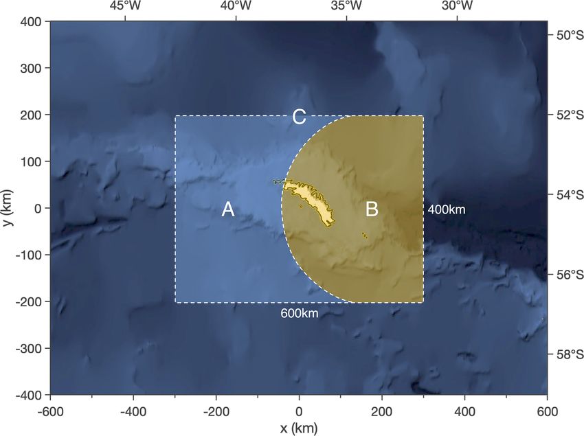
The spatial extent of these three datasets is shown in exhibited more realistic values than the 70-level simulation at
Fig. 1. South Georgia is located around 2000 km east of high altitudes. Therefore, the 118-level configuration is se-
South America and the Antarctic Peninsula in the Southern lected to reduce the computational load and permit the use
Ocean. The 1200 km × 900 km local-area modelling simula- of a fine horizontal grid over the island. It should be men-
tion over the island is shown by the light blue box in Fig. 1a, tioned that although this vertical grid spacing is sufficient to
while the two dashed red and white boxes show two example resolve wintertime orographic waves over South Georgia, the
overpasses of the AIRS instrument (one during an ascend- vertical grid spacing of around 1.5–2 km in the upper strato-
ing node orbit and one during a descending node). Note that sphere is unlikely to accurately simulate body forces under
the exact location of each of the overpasses varies with each wave breaking that are necessary for secondary GW genera-
orbit, as discussed below. Figure 1b and c show 3-D views tion (e.g. Becker and Vadas, 2018). The Unified Model uses
of these domains, through which the trajectories of radioson- a semi-Lagrangian dynamical core, so there is some implicit
des launched from the island during January and June–July numerical diffusion as a result of the interpolation methods
2015 are shown by dashed orange and green lines respec- used to determine the departure points. In the local-area sim-
tively. Note that the June–July radiosondes travelled much ulations used here, the “Smagorinsky-type” 3-D subgrid hor-
further downwind due to stronger stratospheric zonal winds izontal turbulence scheme is used (e.g. Pearson et al., 2014;
during austral winter, and many of these travelled so far east Boutle et al., 2014, and citations therein).
that they exited the local-area model domain. Meteorological initial and lateral boundary conditions for
the local-area domain are provided by a global N512 simula-
2.1 Numerical modelling: local-area simulations over tion with 70 vertical levels from the surface to altitudes near
South Georgia 80 km. At latitudes near South Georgia, this global model
has a horizontal grid spacing of 1x ≈ 46 km. This simula-
Here we use model output from specialised high-resolution tion is provided by Met Office operational analyses and re-
runs of the UK Met Office Unified Model using the Even initialised every 24 h, providing hourly forecasts that supply
https://doi.org/10.5194/acp-21-7695-2021 Atmos. Chem. Phys., 21, 7695–7722, 2021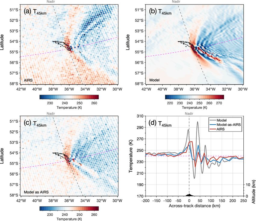
7698                           N. P. Hindley et al.: Gravity waves over South Georgia: modelling and satellite observations

Figure 1. Maps showing the horizontal and vertical extent of the local-area model (blue lines) over the island of South Georgia and two
examples of the typical extent of AIRS satellite measurements (dashed red and white lines) used in this study. Panel (a) shows a map of the
local region around South Georgia, plotted on a regular distance grid. Panels (b and c) show the vertical extent of the model on a latitude–
longitude grid. The vertical extent of usable temperature data from the 3-D AIRS retrieval scheme of Hoffmann and Alexander (2009) is
shown in dashed red lines for both an ascending (b) and descending (c) overpass. Orange (green) lines show the trajectories of radiosondes
launched from the island during a summer (winter) campaign in January (June–July) 2015.

lateral boundary conditions for the local-area configuration               Here we use 3-D AIRS temperature measurements de-
over South Georgia. At the edges of the local-area domain,              rived using the retrieval scheme of Hoffmann and Alexan-
these hourly forecasts are linearly interpolated in time to the         der (2009). This retrieval uses multiple 4.3 and 15 µm CO2
time step of the local-area model (30 s). As mentioned above,           spectral channels to produce estimates of stratospheric tem-
no orographic or non-orographic GW parameterisations were               perature for each individual measurement footprint on a 3 km
included in the local-area simulations. Output fields were              vertical grid. For each height level, retrieved temperatures
archived hourly. More information on the configuration of               have a vertical resolution related to the kernel functions of
these simulations is described in detail by Vosper (2015),              the selected AIRS channels used, which varies between 7–
Vosper et al. (2016) and Jackson et al. (2018).                         14 km for altitudes between 20 and 60 km (Hoffmann and
   The model run used here is for two time periods: 1 to 31             Alexander, 2009; Hindley et al., 2019). The retrieval is opti-
July 2013 and 11 June to 8 July 2015. These austral win-                mised for GW analysis, where a balance is achieved between
tertime periods were chosen to coincide with the high prob-             retrieval noise and vertical resolution. At high southern lati-
ability of strong orographic GW forcing and deep vertical               tudes during winter, temperature measurement error is typi-
propagation due the strong prevailing winds at these lati-              cally .1.5 K (Hoffmann and Alexander, 2009; Hindley et al.,
tudes during winter. A third model run for January 2015 was             2019). Validation of the 3-D AIRS temperature retrievals is
also conducted and analysed, but due to the weak strato-                described by Hoffmann and Alexander (2009) and Meyer and
spheric winds during austral summer, too few GWs (oro-                  Hoffmann (2014).
graphic or non-orographic) were visible in AIRS measure-                   There are typically two AIRS/Aqua overpasses per day
ments for a meaningful comparison. Both model simula-                   over South Georgia, but due to the precession of the orbit,
tions during 2015 were designed to coincide with summer                 the locations of AIRS measurements during each overpass
and winter radiosonde campaigns on South Georgia (Moffat-               are not at the same geographic locations each day. For our
Griffin et al., 2017; Jackson et al., 2018) that are described          study, we select only AIRS overpasses where the measure-
below.                                                                  ment swath covers at least three out of four corners of the
                                                                        local-area model domain, as shown in Fig. 1a. During the
2.2    AIRS 3-D satellite observations                                  model runs in July 2013 and June–July 2015, we found that
                                                                        39 and 48 AIRS overpasses respectively met this three-corner
The Atmospheric Infrared Sounder (AIRS) (Aumann et al.,                 criterion, giving 87 coincident 3-D AIRS measurements in
2003; Chahine et al., 2006) flies aboard NASA’s Aqua satel-             total for our comparison. These overpasses occurred within
lite in a ∼ 100 min near-polar sun-synchronous orbit. AIRS              ±20 min of 03:00 and 17:00 UTC each day and measure-
is a nadir-sounding hyperspectral radiometer that measures              ments typically cover around 80 % to 90 % of the local-area
radiances in 2378 infrared spectral channels in a continu-              model domain due to the high inclination of the AIRS/Aqua
ous 90-element, ∼ 1800 km wide swath in the across-track                orbit.
direction at scan angles between ±49.5◦ from the nadir. The
across-track horizontal spacing of these elements varies from
around 13.5 km at nadir to 41 km at track edge.

Atmos. Chem. Phys., 21, 7695–7722, 2021                                                    https://doi.org/10.5194/acp-21-7695-2021
N. P. Hindley et al.: Gravity waves over South Georgia: modelling and satellite observations                                7699

2.3    Radiosondes                                                ley (2018) showed that a lack of observations can result in
                                                                  significant stratospheric biases in this region in global mod-
We also use wind measurements from radiosonde campaigns           els. The radiosonde measurements described here are not as-
that took place on South Georgia during January (austral          similated into the operational analysis. Thus, to our knowl-
summer) 2015 and June–July (austral winter) 2015, the de-         edge, these radiosonde observations are the only coincident
tails of which are described by Moffat-Griffin et al. (2017).     and independent wind measurements available to assess the
Balloons were launched twice daily from the British Antarc-       tropospheric wind fields in the model over the island during
tic Survey base at King Edward Point (54.3◦ S, 37.5◦ W),          our period of study.
equipped with Vaisala RS92-SGP radiosondes, with addi-               Figure 2 shows hourly zonal and meridional wind against
tional launches timed to coincide with AIRS overpasses            height for the two model runs during July 2013 and June–
or when forecasts predicted strong winds suitable for GW          July 2015. These values are horizontally averaged over the
generation. Meteorological and geolocation parameters are         whole model domain, so they are representative of the large-
recorded at 2 s intervals during the flight.                      scale background flow. As would be expected for a winter-
   The trajectories of the balloons are shown by the orange       time study at these latitudes, wind speeds in the zonal direc-
and green lines in Fig. 1b and c. Fifty-four balloons were suc-   tion are eastward and generally increase strongly with height,
cessfully launched during the wintertime period of 13 June to     with values reaching 120 m s−1 above 50 km altitude. In the
6 July 2015. Due to challenging local environmental condi-        meridional direction, frequent changes between northward
tions, 10 launches failed to reach the tropopause and only 20     and southward flow are observed, with speeds reaching val-
reached altitudes of 25 km or above. During summer, nearly        ues near ±40 m s−1 above 40 km altitude. Gravity wave ac-
all of the 44 balloons launched reached their target altitudes    tivity in the model for this time period is shown in panels e
near 35 km during January 2015. It can also be seen in Fig. 1c    and f discussed later in Sect. 4.
that during winter the balloons travelled much further down-         To compare the model winds to radiosonde observations,
wind to the east than in summer due to the strong westerly        each radiosonde trajectory is traced through the hourly model
wintertime winds. Several balloons were blown so far that         winds fields. Because of the large horizontal distances trav-
they even travelled beyond the eastern boundary of the model      elled by the radiosondes (up to 600 km) and the length of the
domain, 600 km to the east, before reaching their final alti-     flight times (up to around 2.5 h), it is necessary to evaluate
tude. Wind measurements from these balloons are used to           the hourly model data along a path that varies in horizontal
validate the direction and magnitude of the background wind       space, height and time. To do this, all hourly model outputs
in the local-area model to assess conditions for orographic       are loaded for the duration of each radiosonde flight, includ-
GW generation and propagation. A comparison for both the          ing 1 h before and 1 h after, and four-dimensional linear inter-
summer and winter campaigns was performed, but due to re-         polants (x, y, z, t) of zonal u and meridional v wind fields are
duced stratospheric GW activity in the model during sum-          constructed. These interpolants are then evaluated for each
mer, only a comparison for the wintertime measurements is         point along the radiosonde’s trajectory using the measured
shown below.                                                      time, height and location of the balloon. This approach al-
                                                                  lows us to compensate for any time-varying effects in the
                                                                  model wind speeds during the radiosonde flights. The model
3     Model wind validation using co-located radiosonde           winds along the radiosonde trajectories (denoted as model-
      measurements                                                as-sondes hereafter) are then compared to the radiosonde
                                                                  wind observations themselves. Figure 3a shows the results of
Before we compare our simulated GW fields to satellite ob-        our wind comparison. Radiosonde launch times (UTC) and
servations, we first use our co-located radiosonde observa-       maximum recorded altitudes during the winter campaign are
tions to validate the model wind fields. Surface wind flow        shown by the black lines and circles in Fig. 3a. For illustra-
over orography is the key driver of mountain wave activity        tion, the mean zonal wind speed over the modelling domain
over the island (e.g Alexander and Grimsdell, 2013; Vosper,       against altitude in also shown in panel a, which gives us an
2015; Moffat-Griffin et al., 2017; Jackson et al., 2018), and     indication of the background wind conditions through which
upper tropospheric and stratospheric winds determine the          the balloons travelled.
upward propagation of these orographically forced waves.             As can be seen in Fig. 3a, several of the radiosonde bal-
Thus, model winds should first be tested to ensure they are       loons did not reach their desired altitudes near 30 km, in-
a fair representation of reality before any GW investigations     stead bursting soon after launch. This was usually due to the
are undertaken.                                                   extreme weather conditions at low altitudes during the field-
   The boundary conditions of the local-area model are ini-       work campaign, as reported by the radiosonde launch team.
tialised daily by Met Office operational analyses, but these      In some cases, surface winds were so strong that radiosonde
winds are poorly constrained by conventional observations         balloons did not ascend fast enough to exit the bay around
over the Southern Ocean, relying largely on temperatures          the launch site, colliding instead with the slopes of nearby
nudged by assimilated satellite radiances. Wright and Hind-       mountains.

https://doi.org/10.5194/acp-21-7695-2021                                           Atmos. Chem. Phys., 21, 7695–7722, 2021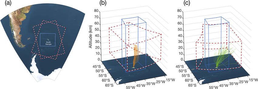
7700 N. P. Hindley et al.: Gravity waves over South Georgia: modelling and satellite observations
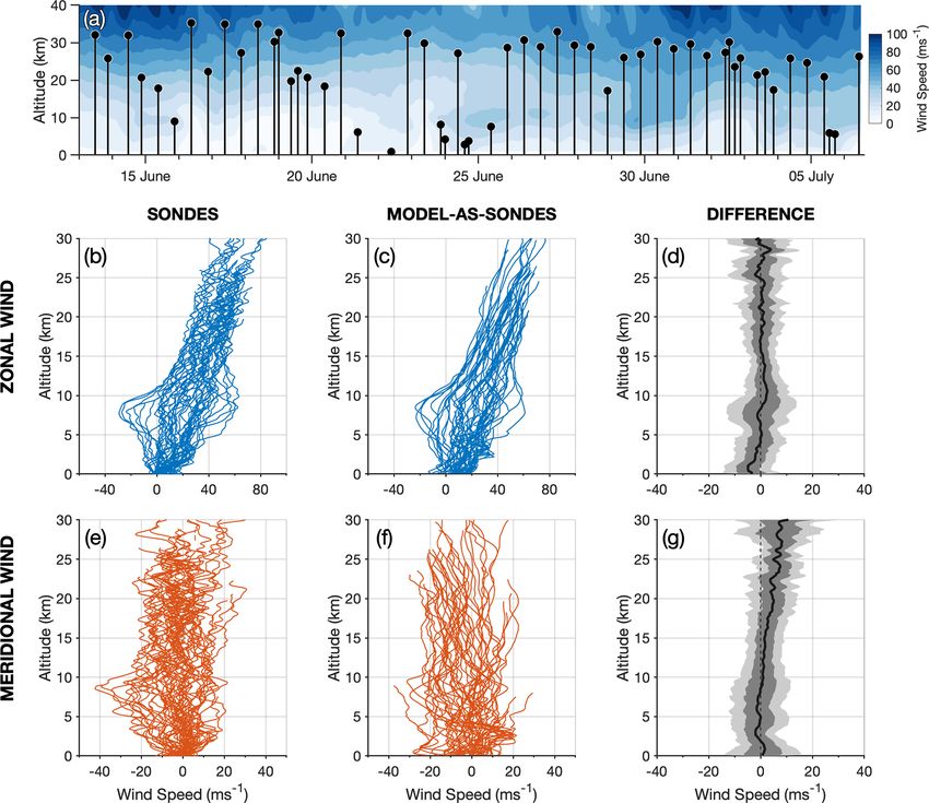
Figure 2. Hourly zonal and meridional wind speeds against altitude in the local-area model over South Georgia during July 2013 (a, c)
and June–July 2015 (b, d) averaged over a horizontal region 600 km × 400 km centred on the island (region
C in Fig. 4). Panels (e, f) show
0 0 0 0
average zonal (blue) and meridional (orange) gravity wave momentum fluxes (GWMFs) ρ u w , v w over the same horizontal region but
between 25 and 45 km altitude. Positive (negative) values indicate eastward (westward) zonal GWMF and northward (southward) meridional
GWMF. Dotted lines in (e, f) show the percentage of the total model GWMF (right axis) downwind of the island (region B in Fig. 4), which
is a strong indication of mountain wave activity.
Panels b–g in Fig. 3 show the measured radiosonde wind 1 and 2 standard deviations of all differences respectively,
speed and the model wind speed evaluated along the ra- while the thick black line shows the mean difference for the
diosonde paths (model-as-sondes) in the zonal and merid- June–July 2015 run.
ional directions. The two datasets are in good general agree- In the zonal direction, the time-averaged difference in
ment, with measured and simulated zonal winds in Fig. 3b wind speed is less than 5 m s−1 for most altitudes above
and c increasing from a few metres per second near the sur- 10 km and close to zero in the low to mid-stratosphere be-
face to around 60 m s−1 near 30 km altitude. In the merid- tween 15 and 25 km altitude. The largest differences between
ional direction, both datasets show wind speeds between the sonde and model-as-sonde winds are seen for altitudes
around ±15 m s−1 with little variation with altitude in Fig. 3e below 10 km in Fig. 3d. This is near the tropopause and could
and f. The radiosonde measurements are found to exhibit suggest that short-timescale variability of the tropospheric
more small-scale variability than the model fields, likely due jet observed over the island is not so well represented in
to small-scale wave or turbulence features and measurement the model. This could influence the upward propagation of
errors which are not present in the model. Some instances mountain waves. Near the surface, below altitudes of around
are also found where sonde measurements are present but no 3 km, a slight bias towards stronger zonal winds in the model
model-as-sonde data are available, which is due to the bal- is observed. We suspect that this is due to slight underrep-
loons horizontally exiting the model domain (see Fig. 1c). resentation of the “roughness” of the complex local topo-
To further compare the simulated and measured wind graphic features around the launch site in the model. King
speeds, the difference between the sonde and the model-as- Edward Point is located in a sheltered bay 2 km east of the
sonde winds (the former minus the latter) against altitude is main mountain ridge of the Thatcher Peninsula, which peaks
shown in Fig. 3d and g for the zonal and meridional direc- at nearly 2 km high. At the 1.5 km model horizontal resolu-
tions respectively. Shaded dark and light grey regions show tion used in this study, this mountain ridge will be at most
Atmos. Chem. Phys., 21, 7695–7722, 2021 https://doi.org/10.5194/acp-21-7695-2021
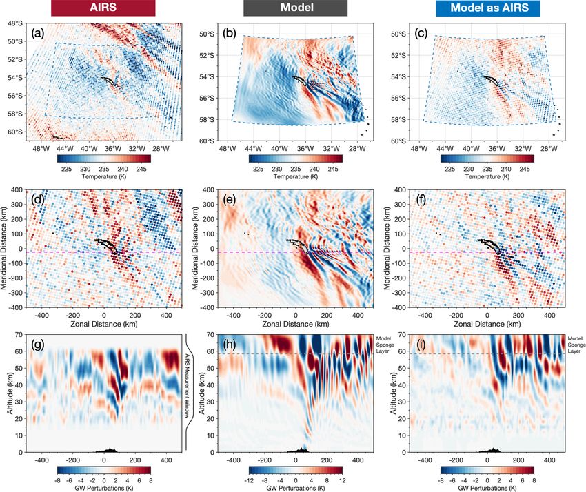
N. P. Hindley et al.: Gravity waves over South Georgia: modelling and satellite observations                                         7701

Figure 3. Comparison of wind speeds from the local-area model to coincident radiosonde observations launched from South Georgia during
June–July 2015. Panel (a) shows launch times and maximum altitudes of the radiosonde observations (black lines), while coloured contours
show the magnitude of the model wind speed for illustration. Panels (b, e, c, f) show profiles of zonal (blue) and meridional (orange) wind
against height for the radiosonde measurements and the model wind, where the model wind has been evaluated along each radiosonde’s
trajectory. Panels (d, g) show the mean difference (thick black line) between the radiosonde and model wind speeds (the former minus the
latter) for each height, while dark grey and light grey shading indicates 1 and 2 standard deviations respectively.

one model grid cell away from the launch site. Thus, accu-              we do not expect this to affect our results significantly, we ac-
rately simulating surface winds at this site will be quite chal-        knowledge that a difference in the rotation of the simulated
lenging. Further, the model winds are not well constrained              wind vector compared to reality could have an effect on wave
by surface observations in the area, so small surface biases            propagation and thus the measured orientations of simulated
are to be expected.                                                     mountain waves over the island.
   In the meridional direction, the time-averaged wind speed               It should be mentioned that some of the differences be-
differences are generally less than 10 m s−1 in Fig. 3g. How-           tween the model and model-as-sonde winds could be due
ever, a clear positive difference is observed above around              to timing or lag issues in the model, such as in the arrival
15 km altitude, which increases to near 10 m s−1 at 30 km al-           of synoptic systems. Anecdotal reports from the radiosonde
titude. This indicates that the model slightly overestimates            launch team on South Georgia suggested that the arrival of
(underestimates) the southward (northward) winds in the                 synoptic systems such as fronts and weather systems could
mid-stratosphere. Because the mean difference is zero for the           differ from the Unified Model forecast by several hours. Al-
zonal component, this then not only tends in a small direc-             though these are tropospheric phenomena, they may have a
tional bias but also in a small positive bias in the net horizon-       stratospheric response that is earlier or later than predicted.
tal wind speed. Given that global models are very poorly con-           These would manifest as pseudo-random errors in our analy-
strained by conventional observations at high southern lati-            sis, which could explain some of the spread in the wind speed
tudes, this directional bias is actually quite reasonable. While        differences. Aside from these differences, however, we con-

https://doi.org/10.5194/acp-21-7695-2021                                                  Atmos. Chem. Phys., 21, 7695–7722, 2021
7702                             N. P. Hindley et al.: Gravity waves over South Georgia: modelling and satellite observations

clude that overall the model wind speed and direction over
the island is simulated reasonably well during the June–July
2015 campaign.
   Caution should be taken when measuring gravity wave
momentum fluxes from slanted vertical profiles through
mountain wave fields (such as radiosonde measurements
here). The usual assumptions required for the measure-
ment of vertically integrated momentum fluxes of planar
monochromatic waves do not hold true for mountain waves
sampled with a slanted vertical profile (e.g. de la Torre and
Alexander, 1995; de la Torre et al., 2018; Vosper and Ross,
2020). For this reason, we do not conduct a GW comparison
between the model and the radiosonde measurements here
and only use the radiosonde measurements to validate the
model winds.

                                                                   Figure 4. Illustration of the two regions to the east and west of
4   Gravity waves over South Georgia in the                        South Georgia used to produce the values in Table 1. Region A is
    full-resolution model                                          upwind of the island and region B is over and downwind of the
                                                                   island. The two regions have equal area.
After validating the simulated winds in our local-area model,
we now consider simulated GW activity in the model. A key
quantity in GW research is the vertical flux of horizontal         generally coincide with periods of increased winds speeds
pseudo-momentum, generally referred to as momentum flux.           from the surface through to the mid-stratosphere, as shown
This property helps to quantify the vertical transfer of hori-     in Fig. 2a–d. This is indicative of strong mountain wave forc-
zontal momentum by GWs. When a GW breaks, horizontal               ing by the surface winds and strong upper tropospheric and
momentum will be deposited in the mean flow, resulting in a        stratospheric winds that combine to provide good conditions
drag or driving effect on the background wind. Measuring           for mountain wave propagation to greater heights. Indeed,
and quantifying the momentum fluxes of mountain waves              during periods shown in Fig. 2a and b where the surface
from small, isolated islands is an important area of current       zonal winds are weak, stratospheric GWMF in Fig. 2e and
research (McLandress et al., 2012; Alexander and Grimsdell,        f is low.
2013; Garfinkel and Oman, 2018; Jackson et al., 2018).                The average zonal direction of GWMF is generally west-
   Figure 2e and f show zonal and meridional gravity wave          ward, which is consistent with what we would expect for
momentum flux (GWMF) averaged between 25 and 45 km                 a mountain wave propagating against the background zonal
altitude and over a horizontal area 600 km × 400 km centred        wind in Fig. 2a. Interestingly, the area-averaged meridional
on the island, denoted by region C in Fig. 4. Here, zonal          GWMF is generally southward, regardless of the direction
GWMF Fx and meridional GWMF Fy are calculated as                   of the background meridional wind. For a typical mountain
                                                                wave over an isolated island source, a characteristic bow-
 Fx , Fy = ρ u0 w0 , v 0 w 0 ,                              (1)    wave pattern is formed that has GWMF directed opposite
                                                                   to the wind but with additional northward and southward
where ρ is the background atmospheric density; u0 , v 0 , and      GWMF to the north and south. The distribution of GWMF
w0 are wind perturbations in the zonal, meridional, and verti-     around the island, shown later in this study, indicates that the
cal directions; and the overbar denotes an area average over       southward component of this mountain wave field over the
GW scales (Fritts and Alexander, 2003; Ern et al., 2004).          island (e.g. Alexander et al., 2009; Alexander and Grimsdell,
Wind perturbations u0 , v 0 and w 0 are separated from the         2013) is considerably larger than the northern component,
background flow by subtracting a fourth-order polynomial fit       likely due to the orientation of the island with respect to the
in the zonal direction. This ensures reasonable consistency        background wind, which results in a southward area-average
with the method used for the AIRS satellite observations de-       overall.
scribed in Sect. 2.2, but the two methods are not identical and       Dotted grey lines (right axes) in Fig. 2e and f show the per-
                                                                                                                      1
therefore should be considered separately.                         centage of the total absolute GWMF (Fx2 + Fy2 ) 2 in region C
   Zonal and meridional GWMF time series in Figs. 2e and f         contained within region B, located downwind of the island
indicate that stratospheric GW activity over the island in the     as shown in Fig. 4. Regions A and B have areas equal to half
full-resolution model is intermittent, with bursts of GWMF         of region C, so a value of 50 % indicates a uniform distribu-
up to around 60 mPa occurring during 7–11 July 2013, 24–           tion of GWMF between the upwind and downwind regions
30 July 2013 and 4–6 July 2015. These bursts of GWMF               to the west and east of the island. A fraction larger than 50 %

Atmos. Chem. Phys., 21, 7695–7722, 2021                                              https://doi.org/10.5194/acp-21-7695-2021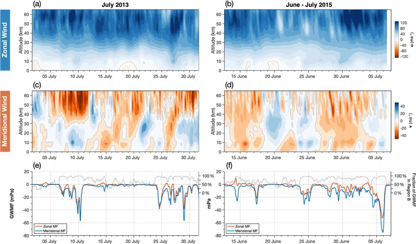
N. P. Hindley et al.: Gravity waves over South Georgia: modelling and satellite observations                               7703

indicates more GWMF in the downwind region, which is a            Table 1). The horizontal sampling distance between the cen-
strong indication of mountain wave activity. It can be seen       tres of these footprints increases with increasing distance
that during nearly all of the periods of increased GWMF in        from the nadir from around 13.5 to 42 km near the track edge,
the model, this fraction is close to around 75 % to 100 %,        so it is important to consider this for GWs with relatively
which suggests that mountain waves are the dominant source        short horizontal scales, such as those expected directly over
of GW activity in the local-area model. This fraction rarely      South Georgia.
falls below 50 % and when it does it is during periods of low        To simulate the AIRS measurement footprints in the
GWMF. This suggests that, relatively, non-orographic GW           model, each vertical level of each model temperature field
activity makes only a small contribution to the GWMF in the       is convolved with a horizontal Gaussian function with a full
local-area model at full resolution.                              width at half maximum (FWHM) equal to 13.5 km×13.5 km.
                                                                  We then interpolate the smoothed model temperatures onto
                                                                  the horizontal sampling grid of the AIRS overpass that is
5     Applying the AIRS observational filter to the model         closest in time to each hourly model output. The Gaussian
                                                                  smoothing step above ensures that this is a reasonable ap-
The GWMF results in the previous section indicate signif-         proximation to the horizontal sampling of an AIRS measure-
icant GW activity in the full-resolution model. But these         ment footprint wherever the model is sampled. This gives us
results cannot be directly compared to AIRS satellite mea-        model temperatures at the horizontal sampling and resolu-
surements, because GW measurements in AIRS are sub-               tion of the nearest coincident AIRS overpass to each hourly
ject to the AIRS observational filter. The observational fil-     model output.
ter (Preusse et al., 2002; Alexander and Barnet, 2007) is
a key concept in GW observations. No single instrument            5.2   Vertical resolution
or technique can measure the full GW spectrum. For ex-
                                                                  Next, we consider the vertical resolution of the AIRS mea-
ample, the standard retrievals of nadir-sounding instrument
                                                                  surements. To apply this vertical resolution to the model, we
such as AIRS will generally have relatively low vertical res-
                                                                  first need to interpolate the model onto a regular vertical
olution (1Z ≈ 15–20 km) for GWs in the stratosphere but
                                                                  grid. The chosen grid is from the surface to 75 km altitude
relatively high horizontal resolution (1L ≈ 50–100 km). In
                                                                  in 1.5 km steps. This grid spacing is finer than the model ver-
contrast, limb-sounding instruments and techniques such as
                                                                  tical grid in the stratosphere but coarser in the troposphere.
HIRDLS (e.g. Gille et al., 2003) or GPS radio occultation
                                                                  Because our comparison to AIRS measurements takes place
(e.g. Kursinski et al., 1997) will have relatively high verti-
                                                                  in the stratosphere, this choice will not significantly affect
cal resolution (1Z ≈ 1 km) but relative low horizontal reso-
                                                                  our results.
lution (1L ≈ 150–270 km). To make a fair comparison be-
                                                                     The vertical resolution of the 3-D AIRS retrieval for dif-
tween GWs in our local-area model and coincident AIRS
                                                                  ferent atmospheric conditions is shown in Fig. 2 of Hindley
satellite observations, we must ensure that both datasets have
                                                                  et al. (2019), where resolution values are derived using the
the same observational filter.
                                                                  approach of Hoffmann and Alexander (2009). The vertical
   For satellite observations, the observational filter is pri-
                                                                  resolution varies, on average, between 7 to 14 km between 20
marily dependent upon two things: sampling and resolution
                                                                  and 60 km altitude. Using the values shown by Hindley et al.
(Wright and Hindley, 2018). Below, we describe how we ap-
                                                                  (2019), we apply the AIRS vertical resolution to the model
ply the sampling pattern and resolution of the AIRS observa-
                                                                  temperature fields. This is a step-by-step process which in-
tions to the local-area model to create a model-sampled-as-
                                                                  volves the convolution of the model temperatures with ver-
AIRS dataset that is comparable to the satellite observations.
                                                                  tical Gaussian functions with different FHWMs for each al-
5.1    Horizontal sampling                                        titude. For example, the vertical resolution at 30 km altitude
                                                                  is approximately 7.5 km (Hindley et al., 2019, their Fig. 2b)
To create the model-sampled-as-AIRS dataset for our com-          so the full 3-D temperature volume is convolved with a verti-
parison to AIRS observations, we use hourly temperature           cal Gaussian function with FWHM equal to 7.5 km, and the
output fields from the local-area model. As described above,      horizontal level at 30 km altitude is then extracted and stored
model temperature fields are on a 1.5 km horizontal grid,         separately. This process is performed for each altitude level,
with 118 vertical levels from the surface to near 70 km al-       allowing us to build up a smoothed temperature field, layer
titude.                                                           by layer, for each hourly model output. The result of this pro-
   The first step is to simulate the AIRS horizontal footprint    cedure is a 3-D volume of model temperatures sampled on
and sampling pattern. The AIRS sampling pattern is well il-       the AIRS horizontal scan track and smoothed to the AIRS
lustrated in Hoffmann et al. (2014, their Fig. 2). AIRS mea-      vertical resolution.
surements are made on a 90-element wide horizontal across-
track swath, where each measurement footprint is approxi-
mately 13.5 km × 13.5 km wide (Hoffmann et al., 2014, their

https://doi.org/10.5194/acp-21-7695-2021                                           Atmos. Chem. Phys., 21, 7695–7722, 2021
7704                         N. P. Hindley et al.: Gravity waves over South Georgia: modelling and satellite observations

5.3    Retrieval noise                                               To extract GW temperature perturbations at each altitude
                                                                  level, a horizontal fourth-order polynomial fit is performed in
Finally, we consider the effect of AIRS retrieval noise. Noise    the across-track direction for each cross-track row (e.g. Wu,
in AIRS measurements can arise due to thermal noise in the        2004; Alexander and Barnet, 2007; Hoffmann et al., 2014;
AIRS instrument and/or deviations of the atmospheric state        Wright et al., 2017; Hindley et al., 2019). Slowly varying
from local thermodynamic equilibrium, which is assumed in         background signals due to large-scale temperature gradients
the retrieval (Hoffmann and Alexander, 2009). These factors       or planetary wave activity are contained in this fit. This is
vary for different spectral channels in the AIRS instrument,      then subtracted from each cross-track row to reveal residual
and as a result the estimated retrieval noise varies between      GW perturbations.
1.2 and 1.5 K between 25 and 45 km altitude, as shown in             As a result of the steps above, our AIRS and model-
Fig. 2a of Hindley et al. (2019) and Fig. 5 of Hoffmann           sampled-as-AIRS temperature perturbations are sensitive to
and Alexander (2009). However, because the retrieval noise        GWs with vertical wavelengths between 8.λz .40 km, as
is pseudo-random and incoherent in the horizontal, coher-         defined by the AIRS vertical resolution. In the horizontal, the
ent wave features at large horizontal scales with amplitudes      sensitivity cutoff for short horizontal wavelengths is deter-
slightly below these noise values can be detected under rea-      mined by the AIRS footprint spacing (2 × 13.5 km = 27 km
sonable conditions (Hindley et al., 2019). In the general case    at nadir and 2 × 40 km = 80 km at the scan edges). For
however, we cannot routinely separate retrieval noise from        longer horizontal wavelengths, sensitivity falls below 90 %
GW perturbations in AIRS measurements, and so to rule out         for λH &700 km and below 10 % at λH &1400 km as a result
the possibility of retrieval noise affecting our comparison, we   of the fourth-order polynomial background fit (Hoffmann
add specified AIRS retrieval noise to our the model sampled       et al., 2014). Sensitivity functions for the 3-D AIRS retrieval
as AIRS.                                                          to stratospheric GWs can be found in Hindley et al. (2019),
   To apply the AIRS retrieval noise to the model, we select      Hoffmann et al. (2014) and Ern et al. (2017).
an AIRS overpass at 17:00 UTC on 20 June 2015 (granule               Because the AIRS temperature retrieval has reduced ver-
numbers 174 and 175) containing no discernible wave fea-          tical resolution and accuracy outside the height range 20
tures at any altitude level. Once the background temperature      to 60 km altitude (Hoffmann and Alexander, 2009), we set
is removed using the method below, the residual perturba-         AIRS and model-sampled-as-AIRS GW perturbations out-
tions exhibit an approximate standard deviation of around         side this range to zero and apply a half-bell tapering window
0.5 K at 39 km altitude. For each altitude level, the residual    to the upper and lower boundaries. This minimises any im-
noise perturbations from this overpass are randomised and         pact of edge effects in our subsequent spectral analysis.
then added to the model temperature fields for each hourly           Figure 5 shows temperature measurements near 45 km al-
model output to simulate AIRS retrieval noise. The use of         titude from AIRS, the full-resolution model and the model
synthetic random Gaussian noise was considered for this pur-      sampled as AIRS during an AIRS overpass at 03:00 UTC on
pose, but since AIRS noise characteristics vary with altitude,    5 July 2015. Coloured circles in a, c, d, and f show the lo-
we found that using genuine AIRS noise provided more re-          cations and horizontal sampling of the AIRS measurements
alistic results.                                                  footprints for this overpass. The dashed blue line denotes the
                                                                  horizontal boundary of the model domain.
                                                                     Characteristic bow-wave patterns are visible over South
6     Measuring 3-D gravity wave properties
                                                                  Georgia in all three datasets in Figs. 5a–c. These are typi-
To investigate the properties of the GWs over South Georgia       cal of orographic “mountain waves” from a small isolated is-
in our AIRS and model-sampled-as-AIRS datasets, we first          land source. These features are apparent as GW perturbations
extract GW temperature perturbations from the background;         in Fig. 5d–f. Significant fine-horizontal-scale wave structure
then we measure GW properties using the 3-D S-transform           is also visible in the full-resolution model, where tempera-
spectral analysis technique.                                      ture perturbations exceed ±12 K directly over the island. The
                                                                  horizontal scales and amplitudes of GW perturbations in the
6.1    Extracting gravity waves temperature                       AIRS and model-sampled-as-AIRS datasets, however, show
       perturbations                                              good qualitative similarity, with GW amplitudes around 6–
                                                                  8 K over the island in both datasets. The addition of the AIRS
As a result of the steps in the previous section, the tempera-    retrieval noise in the model sampled as AIRS is also apparent
ture data for each hourly model-sampled-as-AIRS output lie        in Fig. 5c and f.
on the same grid as the nearest AIRS overpass. This means            Figure 5g–i show a vertical cut through the AIRS, model
that we can use the same background removal method to ex-         and the model sampled as AIRS temperature perturbations
tract GW temperature perturbations from both datasets. This       along the dashed pink line shown in panels d–f. Both AIRS
is important because it ensures that our analysis method does     and model-sampled-as-AIRS measurements are limited to
not introduce differences in the spectral range of GWs visible    between 20 to 60 km altitude, where the retrieval is most
to each dataset that would invalidate our comparison.             reliable (Hoffmann and Alexander, 2009), but for this ex-

Atmos. Chem. Phys., 21, 7695–7722, 2021                                            https://doi.org/10.5194/acp-21-7695-2021
N. P. Hindley et al.: Gravity waves over South Georgia: modelling and satellite observations 7705 Figure 5. Observed and modelled temperatures (a–c) and temperature perturbations (d–f) at 45 km altitude over South Georgia at 03:00 UTC on 5 July 2015 in AIRS measurements, the full-resolution local-area model and the model sampled as AIRS. Coloured circles in (a, c) and (d, f) indicate the size and locations of the AIRS measurement footprints. The bottom row shows vertical cuts through the temperature perturbations along the dashed pink line in (d–f). See Sect. 5 for details on the model-sampled-as-AIRS data. ample we show the full height range of data in the model 150 km) are qualitatively similar to the wave features found sampled as AIRS for completeness. Westward-sloping GW in AIRS in Fig. 5g. While it is not expected that the phase phase fronts with increasing altitude are found over the is- structure of the mountain wave field in the model and obser- land in each of the datasets. These are characteristic of up- vations should match exactly, the agreement is reasonable. wardly propagating mountain waves subject to eastward pre- This example indicates that the horizontal and vertical scales vailing winds (e.g. Vosper, 2015). Again, the full-resolution of GWs in the model sampled as AIRS show good qualitative model in Fig. 5h exhibits large-amplitude wave structure at agreement with GWs observed in AIRS. short horizontal scales (λH around 30–40 km) over the is- To the north-east of the island in Fig. 5a, a large- land and up to around 300 km to the east. However, once horizontal-scale GW structure is observed in the AIRS mea- the AIRS vertical resolution and horizontal sampling is ap- surements. Close inspection of this example suggests that plied in the model sampled as AIRS (Fig. 5i), these short- the phase fronts shown in the AIRS vertical cut in Fig. 5h horizontal-scale structures are diminished, and the remain- between 300 and 500 km east of the island are part of this ing wave structures with larger horizontal scales (λH ≈ 50– same wave structure. We find that wave structures of this kind https://doi.org/10.5194/acp-21-7695-2021 Atmos. Chem. Phys., 21, 7695–7722, 2021
7706                           N. P. Hindley et al.: Gravity waves over South Georgia: modelling and satellite observations

are commonly observed in AIRS measurements in the region             well et al., 2011; McDonald, 2012; Wright and Gille, 2013;
during winter (e.g. Hindley et al., 2019, their Fig. 1), but their   Alexander, 2015; Sato et al., 2016; Hindley et al., 2016;
origin is unclear (Hendricks et al., 2014). Due to their physi-      Wright et al., 2017; Hindley et al., 2019; Hu et al., 2019a, b;
cal scale and orientation, waves like this example are unlikely      Hindley et al., 2020) and has also been applied in a variety of
to have originated from South Georgia.                               other fields, such as the planetary (Wright, 2012), engineer-
   No clear evidence of this wave is found in the model or           ing (Kuyuk, 2015) and biomedical sciences (e.g. Goodyear
the model sampled as AIRS, but this is not unexpected. The           et al., 2004; Brown et al., 2010; Yan et al., 2015).
global forecast that supplies the lateral boundary conditions           Here we use the N -dimensional S-transform (NDST) soft-
for our local-area model has a coarse vertical grid, with only       ware package as described by Hindley et al. (2019). This
70 vertical levels from the surface to near 80 km, so GWs            version builds on the work of previous multidimensional S-
such as this one are unlikely to be accurately simulated. Fur-       transform analysis by Hindley et al. (2016) and Wright et al.
thermore, even if they are accurately simulated, it is not clear     (2017) but applies a superior wave amplitude measurement
how realistically these GWs would be transferred through             technique and features a much faster computational method-
the model boundary conditions into the local-area model. As          ology which reduces computation time by around a factor
a result, we expect our model and model-sampled-as-AIRS              of 10 compared to previous 3DST versions for AIRS analy-
temperature fields to underrepresent GWs of this kind. This          sis. A step-by-step guide describing how the 3DST method is
is discussed further in Sect. 9.                                     applied to 3-D AIRS measurements is described in Hindley
                                                                     et al. (2019, their Sect. 3).1 Validation of the 3DST analysis
6.2    Measuring gravity wave properties with a 3-D                  method using synthetic wave fields can be found in Hindley
       S-transform                                                   et al. (2016) and Hindley et al. (2019).
                                                                        To make meaningful 3DST measurements of wavelengths,
In Sect. 4 we used directional wind perturbations u0 , v 0 and       a regular orthogonal grid is required. The AIRS and model-
w0 to estimate GW momentum flux in the full-resolution               sampled-as-AIRS datasets have irregular across-track spac-
model via Eq. (1). However, AIRS can only measure GW                 ing (Fig. 5), so we interpolate the GW temperature pertur-
temperature perturbations, so we must use these to make our          bations for each AIRS overpass and each hourly model-
comparison between AIRS and the model sampled as AIRS.               sampled-as-AIRS output onto a 10 km × 10 km horizontal
   We can use spatially localised measurements of GW tem-            grid centred on South Georgia. This is finer than the horizon-
perature amplitudes T 0 , horizontal wavenumbers k and l, and        tal sampling of the AIRS grid, so aliasing effects are unlikely
vertical wavenumber m to estimate directional GWMF in                to be significant. If any aliasing effects do occur, their effects
AIRS and model-sampled-as-AIRS measurements via the re-              will be equal for the AIRS and the model sampled as AIRS,
lation                                                               so this will not affect our comparison. In the vertical, we in-
             ρ  g 2 |T 0 | 2 k l
                                                                 terpolate onto a 1.5 km vertical grid which is finer than the
 MFx , MFy =                           ,    ,               (2)      stratospheric vertical grids (and vertical resolutions) of both
                2 N          T        m m
                                                                     the AIRS retrieval and the model. This regridding is therefore
where MFx and MFy are the zonal and meridional compo-                unlikely to affect our results.
nents of GWMF, ρ is atmospheric density, g is the acceler-              We apply the 3DST to regularly gridded GW tempera-
ation due to gravity, N is the buoyancy frequency, and T is          ture perturbations for 87 three-dimensional AIRS measure-
the background atmospheric temperature (Ern et al., 2004).           ments and 1320 hourly model-sampled-as-AIRS outputs dur-
Zonal, meridional and vertical wavenumbers k, l and m                ing July 2013 and June–July 2015. Following the approach
are related to spatial wavelengths as k = 2π/λx , l = 2π/λy          of Hindley et al. (2019), we set the 3DST scaling param-
and m = 2π/λz respectively. This relation is valid for mid-          eter cx = cy = cz = 0.25 and analyse for the 1000 largest-
frequency GWs, where the intrinsic frequency ω̂2  f 2 ,             amplitude wave signals with wavelengths greater than 27, 27
where f is the inertial frequency (Fritts and Alexander,             and 6 km in the x, y and z directions respectively. These are
2003). Ern et al. (2017) showed that this relation is valid for      Nyquist sampling limits of twice the smallest separation of
GWs within the spectral range visible to AIRS.                       original AIRS sampling pattern (2 km × 13.5 km) in the hor-
   To obtain spatially localised measurements of GW ampli-
                                                                         1 It should be mentioned that the S-transform method of Hindley
tudes and wavelengths, we use a 3-D adaptation of the S-
transform (also known as the Stockwell transform). Devel-            et al. (2019) does not use sets of orthogonal basis functions, as de-
                                                                     scribed for the discrete orthonormal S-transform (DOST) method
oped by Stockwell et al. (1996), the S-transform is a widely
                                                                     of Stockwell (2007). Instead, the Hindley et al. (2019) method is
used spectral analysis technique that can localise and mea-          configured to analyse for all basis functions at all spatial frequency
sure the amplitudes of individual frequencies (or wavenum-           combinations (fx , fy , fz ) at all spatial locations (x, y, z) singly and
bers) in a time series or distance profile. The S-transform          one at a time. In signal-processing terms, this is of course highly re-
has been applied for GW analysis in a variety of geophysical         dundant, but it provides us with the maximum possible spectral and
datasets (e.g. Fritts et al., 1998; Stockwell and Lowe, 2001;        spatial sampling, which is ideally suited for measuring the localised
Alexander and Barnet, 2007; Alexander et al., 2008; Stock-           spectral properties of gravity wave packets in noisy data.

Atmos. Chem. Phys., 21, 7695–7722, 2021                                                  https://doi.org/10.5194/acp-21-7695-2021
You can also read