Declining, seasonal-varying emissions of sulfur hexafluoride from the United States
←
→
Page content transcription
If your browser does not render page correctly, please read the page content below
Research article
Atmos. Chem. Phys., 23, 1437–1448, 2023
https://doi.org/10.5194/acp-23-1437-2023
© Author(s) 2023. This work is distributed under
the Creative Commons Attribution 4.0 License.

                 Declining, seasonal-varying emissions of sulfur
                       hexafluoride from the United States
              Lei Hu1 , Deborah Ottinger2 , Stephanie Bogle2 , Stephen A. Montzka1 , Philip L. DeCola3,4 ,
         Ed Dlugokencky1 , Arlyn Andrews1 , Kirk Thoning1 , Colm Sweeney1 , Geoff Dutton1,5 , Lauren Aepli2 ,
                                               and Andrew Crotwell1,5
         1 GlobalMonitoring Laboratory, US National Oceanic and Atmospheric Administration, Boulder, CO, USA
                  2 Climate Change Division, US Environmental Protection Agency, Washington D.C., USA
            3 Department of Atmospheric and Oceanic Sciences, University of Maryland, College Park, MD, USA
                                         4 GIST.Earth LLC, Washington D.C., USA
                              5 Cooperative Institute for Research in Environmental Sciences,

                                    University of Colorado Boulder, Boulder, CO, USA
                                         Correspondence: Lei Hu (lei.hu@noaa.gov)

                                 Received: 31 August 2022 – Discussion started: 15 September 2022
                        Revised: 30 December 2022 – Accepted: 5 January 2023 – Published: 26 January 2023

       Abstract. Sulfur hexafluoride (SF6 ) is the most potent greenhouse gas (GHG), and its atmospheric abundance,
       albeit small, has been increasing rapidly. Although SF6 is used to assess atmospheric transport modeling and
       its emissions influence the climate for millennia, SF6 emission magnitudes and distributions have substantial
       uncertainties. In this study, we used NOAA’s ground-based and airborne measurements of SF6 to estimate SF6
       emissions from the United States between 2007 and 2018. Our results suggest a substantial decline of US SF6
       emissions, a trend also reported in the US Environmental Protection Agency’s (EPA) national inventory sub-
       mitted under the United Nations Framework Convention on Climate Change (UNFCCC), implying that US
       mitigation efforts have had some success. However, the magnitudes of annual emissions derived from atmo-
       spheric observations are 40 %–250 % higher than the EPA’s national inventory and substantially lower than the
       Emissions Database for Global Atmospheric Research (EDGAR) inventory. The regional discrepancies between
       the atmosphere-based estimate and EPA’s inventory suggest that emissions from electric power transmission and
       distribution (ETD) facilities and an SF6 production plant that did not or does not report to the EPA may be un-
       derestimated in the national inventory. Furthermore, the atmosphere-based estimates show higher emissions of
       SF6 in winter than in summer. These enhanced wintertime emissions may result from increased maintenance of
       ETD equipment in southern states and increased leakage through aging brittle seals in ETD in northern states
       during winter. The results of this study demonstrate the success of past US SF6 emission mitigations and suggest
       that substantial additional emission reductions might be achieved through efforts to minimize emissions during
       servicing or through improving sealing materials in ETD.

1   Introduction                                                   (ETD) equipment; its emissions occur during manufactur-
                                                                   ing, use, servicing, and disposal of the equipment. There is
Sulfur hexafluoride (SF6 ) is the greenhouse gas (GHG) with        also usage and associated emissions of SF6 from the produc-
the largest known 100-year global warming potential (GWP)          tion of magnesium and electronics. Because of its extremely
(i.e., 25 200) and an atmospheric lifetime of 580–3200 years       large GWP and long atmospheric lifetime, emissions of SF6
(Forster et al., 2021; Ray et al., 2017). SF6 is primarily used    accumulate in the atmosphere and will influence Earth’s cli-
in electrical circuit breakers and high-voltage gas-insulated      mate for thousands of years. Since 1978, global emissions
switchgear in electric power transmission and distribution

Published by Copernicus Publications on behalf of the European Geosciences Union.
1438                                        L. Hu et al.: Declining, seasonal-varying emissions of SF6 from the United States

of SF6 have increased by a factor of 4 due to the rapid ex-
pansion of ETD systems and the metal and electronics in-
dustries (Rigby et al., 2010; Simmonds et al., 2020). As a
result, the global atmospheric mole fractions and radiative
forcing of SF6 have increased by 14 times over the same pe-
riod. In 2019, the radiative forcing of SF6 was 6 mW m−2 or
0.2 % of the total radiative forcing from all long-lived GHGs,
making it the 11th largest contributor to the total radiative
forcing among all the long-lived greenhouse gases and the
7th largest contributor among gases whose atmospheric con-
centrations are still growing (i.e., other than chlorofluorocar-
bons (CFCs) and carbon tetrachloride) (Gulev et al., 2021).
If global SF6 emissions continue at the 2018 rate (9 Gg yr−1 )
into the future, the global atmospheric mole fraction and ra-
diative forcing of SF6 will linearly increase by another factor
of 4 by the end of the 21st century (Fig. S1). If global emis-
sions of SF6 continue to rise at the same rate as 2000–2018,
the global atmospheric mole fraction and radiative forcing
of SF6 will increase by another factor of 10 by the end of
the 21st century (Fig. S1). Consistent with the large GWP of
SF6 emissions and its importance for influencing climate for        Figure 1. US SF6 emissions derived from atmospheric observa-
many years, national emissions of this gas are reported un-         tions and reported by inventories. (a) Locations of atmospheric SF6
                                                                    measurements considered in the regional inversions; tower-based
der the United Nations Framework Convention on Climate
                                                                    sampling is indicated as stars and airborne-profile sampling is de-
Change (UNFCCC) annually by the United States. Further-             noted as circles. Sensitivity of the atmospheric SF6 measurements
more, accurate estimates of the magnitude and distribution          to surface emissions is indicated on a log10 scale as purple shading.
of SF6 emissions are also important in studies to refine our        (b) US SF6 emissions reported by EDGAR (v4.2 and v7.0) and EPA
understanding of atmospheric transport processes in the tro-        inventories and derived from atmospheric observations. National to-
posphere and stratosphere (Orbe et al., 2021; Waugh et al.,         tals are shown from EDGARv7.0, whereas the EPA inventory is
2013; Denning et al., 1999; Gloor et al., 2007; Peters et al.,      parsed out by sector, including electric power transmission and dis-
2004; Schuh et al., 2019; Ray et al., 2017; Maiss and Levin,        tribution (ETD), electrical equipment manufacturing (EPM), mag-
1994; Harnisch et al., 1996).                                       nesium production, and electronics. Atmosphere-based emission es-
   Although global emissions of SF6 can be well constrained         timates for the contiguous United States (CONUS) are derived with
with knowledge of its observed remote-atmosphere growth             two different model analyses of the atmospheric observations us-
                                                                    ing two different transport simulations (HYSPLIT–NAMS in purple
rates and its atmospheric lifetime, large uncertainties remain
                                                                    shading for 2008–2018 and WRF–STILT in gray shading for 2007–
in the magnitude and distribution of SF6 emissions on na-           2017). The black line with error bars indicates inversion ensemble
tional and regional scales. For example, the total annual na-       annual means and an uncertainty at a 95 % confidence interval.
tional emissions reported to the UNFCCC summed from its
Annex I (mostly developed countries) and some non-Annex I
(mostly developing) countries (including China, one of the
large SF6 emitting countries) account for only 50 % of global       (US Environmental Protection Agency, 2022a) (Fig. 1). The
annual SF6 emissions derived from atmospheric observa-              causes for this large difference are not fully known but appear
tions for 1990–2007 (Simmonds et al., 2020; Rigby et al.,           to arise largely from the ETD sector (Fig. S2). Uncertainties
2010; Levin et al., 2010). This difference between activity-        in the EPA’s emission estimates were also illuminated by a
based inventory (“bottom-up”) estimates and atmosphere-             comparison between the SF6 usage inferred from the user
based (“top-down”) estimates may result from underesti-             reports (which form the basis of EPA’s emission estimates)
mates of emissions by activity-based inventories (Simmonds          and the SF6 usage inferred from suppliers’ reports, which
et al., 2020; Rigby et al., 2010; Levin et al., 2010; Weiss and     showed that supplier-based estimates were 70 % higher than
Prinn, 2011) as well as from substantial emissions from non-        user-based estimates in 2012 (Ottinger et al., 2015).
reporting countries. The results of activity-based inventories         Against this backdrop, we estimated US SF6 emissions be-
are sensitive to estimated activity levels and, especially, emis-   tween 2007 and 2018 using inverse modeling of atmospheric
sion rates. In the Emission Database for Global Atmospheric         mole fraction measurements made from ground-based and
Research (EDGAR; Janssens-Maenhout, 2011; Crippa et al.,            airborne whole-air flask samples collected from the US Na-
2020), US SF6 emissions were up to 5 times larger than              tional Oceanic and Atmospheric Administration (NOAA)
the emissions estimated by the US Environmental Protec-             Global Greenhouse Gas Reference Network (Fig. 1). The
tion Agency (EPA) and in their reporting to the UNFCCC              analysis provides robust emission estimates by region and

Atmos. Chem. Phys., 23, 1437–1448, 2023                                                https://doi.org/10.5194/acp-23-1437-2023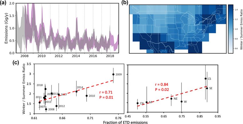
L. Hu et al.: Declining, seasonal-varying emissions of SF6 from the United States                                           1439

season for the contiguous United States (CONUS). Our study        mole fractions that were derived using three different ap-
offers an independent estimate that complements the current       proaches. These approaches are similar to previous inversion
US inventory-based national emission reporting of SF6 to          analyses for other atmospheric trace gases (Hu et al., 2021,
the UNFCCC. This effort exemplifies the quality assurance         2017). In all three approaches, we constructed an empirical
guidance laid out in the 2019 Refinement to the 2006 IPCC         4D mole fraction field based on measurements made in air
Guidelines for National Greenhouse Gas Inventories, which         over the Pacific and Atlantic Ocean basins and in the free
states that “Atmospheric measurements are being used to           troposphere above 3 km over North America, so that it con-
provide useful quality assurance of the national greenhouse       tains vertical and horizontal gradients of mole fractions mea-
gas emission estimates. Under the right measurement and           sured in the remote atmosphere over time. From this empir-
modeling conditions, they can provide a perspective on the        ical background, we then extracted the mole fraction at the
trends and magnitude of greenhouse gas (GHG) emission es-         sampling time and location of each observation and used it
timates that is largely independent of inventories” (Maksyu-      as our first background estimate. In the second approach, we
tov et al., 2019). In fact, the United Kingdom, Switzerland,      considered 500 air back trajectories associated with each ob-
and Australia have already included top-down atmosphere-          servation. Five hundred background estimates were extracted
based emission estimates in the quality assurance and qual-       from this empirical background at the locations where the
ity control (QA/QC) section of their national GHG emis-           air back trajectories exited the North American domain hori-
sion reporting to UNFCCC (Fraser et al., 2014; Henne et al.,      zontally or where they were aloft above 5 km. In most cases,
2016; Manning et al., 2021). The United States also started       the majority of particles exited North America horizontally
to include top-down estimates of four major hydrofluorocar-       or vertically within 10 d, but for those that remained within
bons (HFCs) as a comparison to the US national Greenhouse         the domain after 10 d, background values were derived from
Gas Inventory (GHGI) reporting in 2022 (US Environmen-            their positions 10 d after sampling. For mid-continent and
tal Protection Agency, 2022a). Derived national and regional      eastern sites, there were up to 20 % of particles that remained
SF6 emissions from this analysis are accessible through the       within the domain after 10 d. The 500 background estimates
NOAA’s US Emission Tracker for Potent GHGs website                were averaged to obtain the background mole fraction es-
(https://gml.noaa.gov/hats/US_emissiontracker, last access:       timation for that observation. In the third approach, we as-
19 January 2023).                                                 sessed potential biases in the background estimate from the
                                                                  second approach, particularly because there was a small frac-
                                                                  tion of back trajectories ending up in the planetary boundary
2   Methods                                                       layer in North America after 10 d. Background mole frac-
                                                                  tions for these particles were likely higher than estimated
Top-down atmosphere-based SF6 emission estimates were             using the marine boundary layer information. To minimize
derived using inverse modeling of NOAA’s long-term at-            such biases, we corrected our background estimates from the
mospheric measurements of SF6 (https://gml.noaa.gov/aftp/         second approach based on their differences with measure-
data/hats/sf6/Data_in_Hu_et_al_2023/, last access: 19 Jan-        ments made within North America that had small surface
uary 2023). Measurements made over North America were             sensitivities over populated areas (Hu et al., 2017).
based on air samples collected by discrete flasks from tall          SF6 mole fraction enhancements estimated in observations
towers and aircraft. The tall tower flask samples were typ-       at North American sites were then incorporated into a re-
ically collected every 1 to 2 d (days) and airborne flask-        gional inverse model to estimate US national and regional
sample profiles were collected once or twice per month be-        emissions, following the same methodology as described in
tween 0 and 8 km above sea level. Measurements made out-          our previous inversion studies for other anthropogenic gases
side North America were from weekly whole-air samples             (Hu et al., 2017, 2015, 2016). In regional inversions, we as-
collected globally, generally at remote locations far away        sume a linear relationship between atmospheric mole frac-
from emission sources (https://gml.noaa.gov/dv/site/, last ac-    tion enhancements and upwind emissions. The linear opera-
cess: 19 January 2023). All the whole-air flask samples were      tor is called a “footprint” or the Jacobian matrix, representing
shipped to Boulder and analyzed by gas chromatography             the spatial and temporal sensitivity of atmospheric mole frac-
with an electron capture detector (GC-ECD) for SF6 . Uncer-       tion observations to emissions. Footprints were computed
tainty of each SF6 flask measurement is approximately 0.04        by two transport models, the coupled Weather Research and
to 0.05 ppt, which includes uncertainties related to short-term   Forecasting–Stochastic Time-Inverted Lagrangian Transport
measurement noise, long-term measurement reproducibility,         model (WRF–STILT) (Nehrkorn et al., 2010) and the Hy-
and calibration scale that was transferred from gravimetric       brid Single-Particle Lagrangian Integrated Trajectory model
standards to working standards.                                   (Stein et al., 2015) driven by the North American Mesoscale
   Mole fraction enhancements of SF6 over CONUS (Fig. 1)          Forecast System (HYSPLIT–NAMS). The WRF field has
relative to SF6 mole fractions in air measured upwind were        41 pressure levels and a horizontal resolution of 10 km in
then estimated for deriving US emissions. These enhance-          North America and 40 km outside of North America. The
ments were estimated by referencing them to “background”          NAMS meteorology has a 12 km resolution and 40 sigma-

https://doi.org/10.5194/acp-23-1437-2023                                          Atmos. Chem. Phys., 23, 1437–1448, 2023
1440 L. Hu et al.: Declining, seasonal-varying emissions of SF6 from the United States
pressure levels. Before March 2009, when NAMS was not inversions that have 2 representations of transport, 2 prior
available, we used NAM-12 meteorology, which only has 26 emission fields, and 3 background estimates. Assume µi and
vertical levels. NAMS or NAM-12 was nested with the US σi represent the posterior emission estimate and its associ-
National Centers for Environmental Prediction (NCEP) 0.5◦ ated 1σ error for the ith inversion. Our final estimate of emis-
Global Data Assimilation System (GDAS0.5) with 55 sigma- sions and its associated uncertainty discussed in the text were
pressure levels. Both WRF–STILT and HYSPLIT–NAMS calculated as the mean posterior emission and the 2σ uncer-
were run with 500 particles back in time for 10 d (e.g., Miller tainty (2σt ) derived from Eq. (1):
et al., 2013; Nevison et al., 2018; Miller et al., 2012; Ger- s
big et al., 2003). In each run, particles were released at the σ12 + σ22 + . . . + σ12
2
sampling inlet heights. Footprints were then calculated by σt = + σs2 , (1)
12
integrating particles between the modeled surface to mod-
eled boundary layer in each grid at each time step (Lin et al., where σs denotes 1σ spread or variability of the posterior
2003). emissions derived from all 12 inversions.
A Bayesian inverse modeling technique (Rodgers, 2000)
was implemented, where a prior emission field was re-
3 Results and discussion
quired. The model adjusts magnitudes and distributions of
the prior emissions at a 1◦ × 1◦ × weekly resolution, such
3.1 Declining SF6 emissions from the United States
that the posterior solution of emissions better represents
the observed magnitudes, and horizontal and vertical gradi- The United States recognized that it had significant emis-
ents of mole fraction enhancements observed in the United sions of SF6 in the 1990s and has taken steps to reduce its
States. Here, we used two different temporally constant prior national emissions. In the United States, 60 %–80 % of SF6
emission fields. The first one was from the EDGAR ver- emissions have historically been from the ETD sector (US
sion 4.2 (EDGARv4.2) with a US total SF6 emission of Environmental Protection Agency, 2022a) (Fig. 1). Outside
1.8 Gg yr−1 in 2008. The 2008 EDGARv4.2 estimate was the ETD sector, smaller amounts of SF6 are used in semi-
applied for all years between 2007–2018 in our inversions. conductor manufacturing processes as a source of fluorine
EDGARv4.2 was the most recent grid-scale product offered to etch patterns onto chips and to clean thin film deposition
at the time that we conducted our inversions. EDGAR ver- chambers, and SF6 is also used as a cover gas in magnesium
sion 7.0 (EDGARv7.0) became available only after this work production and casting processes to prevent rapid oxidation
was submitted in late September of 2022. It extends this of molten magnesium. Both of these uses result in emis-
inventory emission through 2021 and its US total and re- sions. SF6 emissions from magnesium processes accounted
gional SF6 emissions for earlier years are similar to those for roughly 15 %–30 % of the US total emissions reported
in EDGARv4.2 (Figs. 1 and 2). Given the similarities of by EPA between 1990 and 2018 (Fig. 1). While the mag-
EDGAR v7.0 with v4.2 in distribution and magnitude, and nitude of SF6 emissions from the electronics manufacturing
the insensitive nature of our posterior results to these as- sector has not changed much over time, its share of total US
pects of the prior (see below), we did not rerun inversions SF6 emissions in the EPA inventory has increased from 2 %
with EDGARv7.0 as prior emissions. The second prior emis- in 1990 to 14 % in 2018 as emissions from other industries
sion field includes a US total emission of 0.4 Gg yr−1 for have decreased.
2007–2018. It was distributed by population density from the Since 1999, the US EPA has worked with the electric
Gridded Population of the World (GPW) v4 dataset (https: power industry through the voluntary SF6 Emission Re-
//sedac.ciesin.columbia.edu/data/collection/gpw-v4, last ac- duction Partnership for Electric Power Systems to identify,
cess: 15 March 2019). The weight between the prescribed recommend, and implement cost-effective solutions to re-
prior emissions and atmospheric observations in the final duce SF6 emissions. There have also been regulations at
posterior emission solution was determined by the values in the state level to reduce SF6 emissions from the ETD sec-
the prior emission error covariance matrix and the model- tor (US Environmental Protection Agency, 2022a). In addi-
observation mismatch covariance matrix, which were calcu- tion, the EPA operated voluntary partnership programs with
lated from the maximum likelihood estimation (Michalak et the semiconductor and magnesium industries from the late
al., 2005; Hu et al., 2015). 1990s through 2010 to understand and reduce their emis-
In each inversion, the derived 1◦ × 1◦ × weekly emissions sions. These national- and state-level mitigation strategies,
and emission uncertainties were aggregated to derive emis- along with an increase in the market price of SF6 during
sions and uncertainties at regional and national scales and at the 1990s, have resulted in a substantial reduction in to-
monthly and annual time steps. When calculating the pos- tal US SF6 emissions since 1990 (Fig. 1). In addition, be-
terior uncertainty, we considered the temporal and spatial fore 2011, SF6 was likely emitted from an SF6 production
correlations of posterior errors in the derived full posterior plant that ceased the production of SF6 in 2010, according
emission covariance matrix. The final reported emissions to data reported to the US EPA. Total US SF6 emissions
and emission uncertainties include results from a total of 12 estimated by the EDGARv4.2 or EDGARv7.0 inventories
Atmos. Chem. Phys., 23, 1437–1448, 2023 https://doi.org/10.5194/acp-23-1437-2023L. Hu et al.: Declining, seasonal-varying emissions of SF6 from the United States 1441 Figure 2. Regional SF6 emissions over the United States, derived from atmospheric observations and reported by EPA’s GHGI and EDGAR (EDGARv4.2 and EDGARv7.0). EPA emissions are parsed out by sectors, i.e., electrical power transformation and distribution (ETD), elec- trical power manufacturing (EPM), magnesium production, and electronics, while EDGAR emissions are presented as totals. Atmosphere- based emission estimates (black lines) include uncertainties at a 95 % confidence interval (vertical black bars). showed an absolute decline over this period similar to that based estimate and EDGARv7.0 increases over time, in the EPA National Greenhouse Gas Inventory, but EDGAR whereas the difference between the atmosphere-derived es- emissions were substantially larger on average (Fig. 1). Note timate and EPA’s inventory decreases over time. After 2011, that although the US national total in EDGARv7.0 suggests the atmosphere-based emission estimates are 0.93 (±0.07, lower emissions than EDGARv4.2, this difference arises 2σ ) Gg yr−1 (a factor of 3.4) lower than EDGARv7.0 and only in the magnesium production sector. There were slightly only about 0.15 (±0.07, 2σ ) Gg yr−1 (35 %) higher than the higher emissions from the ETD and electronics industries EPA’s GHGI (US Environmental Protection Agency, 2022a). in EDGARv7.0 than in EDGARv4.2 over the United States The improved agreement between the EPA GHGI and the (Fig. S2). atmosphere-based estimates may be associated with more ac- Consistent with the inventory reports, the independent, curate emission information used to inform the EPA’s GHGI atmospheric observation-based results presented here sug- after 2010. Before 2011, the SF6 emission estimate in the gest a large decline of US total SF6 emissions, confirm- EPA GHGI was primarily informed by reporting through ing the success of US SF6 emission mitigation efforts. the voluntary partnership programs between EPA and vari- The atmospheric observation-based emissions declined from ous industries (Rand, 2012) described above. In 2011, EPA 0.93 (±0.19, 2σ ) Gg yr−1 in 2007–2008 to 0.37 (±0.10, established its Greenhouse Gas Reporting Program (GH- 2σ ) Gg yr−1 in 2017–2018 (Table 1 and Fig. 1). The 0.56 ± GRP), requiring facility-based reporting of GHG data and 0.21 (2σ ) Gg yr−1 drop in SF6 emissions from 2007–2008 other relevant information from large GHG emission sources to 2017–2018 is equivalent to a reduction of 13 ± 7 × 10⁶ t (≥ 25 000 CO2 -equivalent metric tons of GHG emissions per (metric tons) of CO2 emissions when using the 100-year year). Although smaller emitters are not required to report global warming potential that was used in the EPA GHGI their emissions, this program provides more complete emis- (GWP100 = 22 800). sion information than had been available prior to 2011. For Although both the atmosphere-based top-down and example, from 1999 to 2010, ETD facilities representing an inventory-based bottom-up estimates show declining trends estimated 60 % of the emitting activity reported their SF6 for total US SF6 emissions, the estimated emission mag- emissions to EPA through EPA’s voluntary reporting pro- nitudes are quite different. In 2007–2008, the atmosphere- gram. After 2010, ETD facilities representing an estimated based emissions fell between the EDGARv7.0 and EPA’s 70 % of the emitting activity began reporting their emissions GHGI estimates, but the difference between the atmosphere- to EPA under the GHGRP. https://doi.org/10.5194/acp-23-1437-2023 Atmos. Chem. Phys., 23, 1437–1448, 2023
1442                                                L. Hu et al.: Declining, seasonal-varying emissions of SF6 from the United States

Table 1. US national and regional annual emissions of SF6 (in Gg yr−1 ) reported by EPA and derived from NOAA atmospheric measure-
ments from this study. Errors derived from NOAA atmospheric measurements are expressed at a 95 % confidence interval.

                                                                                             Regions
          National totals
 Year
                                    Northeast              Southeast         Central north             Central south            Mountain               West
        EPA         NOAA     EPA          NOAA      EPA          NOAA      EPA        NOAA       EPA            NOAA     EPA          NOAA      EPA           NOAA
 2007   0.40   0.83 ± 0.19   0.04     0.18 ± 0.10   0.03     0.05 ± 0.07   0.16   0.30 ± 0.07     0.06     0.22 ± 0.07   0.07     0.04 ± 0.03   0.04   0.03 ± 0.07
 2008   0.37   1.03 ± 0.26   0.05     0.22 ± 0.10   0.02     0.09 ± 0.07   0.13   0.34 ± 0.14     0.06     0.28 ± 0.09   0.06     0.06 ± 0.04   0.03   0.04 ± 0.06
 2009   0.32   0.75 ± 0.26   0.04     0.16 ± 0.10   0.03     0.08 ± 0.05   0.10   0.25 ± 0.13     0.06     0.22 ± 0.10   0.06     0.02 ± 0.03   0.03   0.02 ± 0.04
 2010   0.32   0.63 ± 0.16   0.04     0.12 ± 0.04   0.02     0.05 ± 0.03   0.11   0.20 ± 0.08     0.06     0.12 ± 0.04   0.06     0.05 ± 0.02   0.03   0.08 ± 0.04
 2011   0.36   0.58 ± 0.12   0.04     0.13 ± 0.04   0.03     0.06 ± 0.02   0.14   0.19 ± 0.05     0.06     0.11 ± 0.03   0.06     0.03 ± 0.02   0.03   0.06 ± 0.02
 2012   0.30   0.40 ± 0.11   0.04     0.09 ± 0.05   0.03     0.04 ± 0.03   0.10   0.13 ± 0.03     0.05     0.08 ± 0.03   0.05     0.03 ± 0.02   0.03   0.04 ± 0.02
 2013   0.28   0.40 ± 0.12   0.04     0.11 ± 0.07   0.03     0.03 ± 0.03   0.08   0.13 ± 0.04     0.04     0.08 ± 0.03   0.05     0.02 ± 0.02   0.03   0.03 ± 0.02
 2014   0.29   0.48 ± 0.14   0.04     0.15 ± 0.09   0.03     0.05 ± 0.03   0.09   0.13 ± 0.04     0.05     0.08 ± 0.03   0.05     0.03 ± 0.02   0.03   0.03 ± 0.02
 2015   0.24   0.43 ± 0.14   0.04     0.13 ± 0.05   0.02     0.05 ± 0.03   0.08   0.13 ± 0.04     0.04     0.07 ± 0.02   0.04     0.03 ± 0.02   0.02   0.03 ± 0.02
 2016   0.26   0.40 ± 0.09   0.04     0.12 ± 0.04   0.03     0.04 ± 0.02   0.10   0.11 ± 0.03     0.04     0.08 ± 0.04   0.04     0.02 ± 0.02   0.02   0.02 ± 0.02
 2017   0.26   0.35 ± 0.12   0.03     0.09 ± 0.04   0.03     0.03 ± 0.03   0.09   0.10 ± 0.03     0.04     0.08 ± 0.04   0.04     0.03 ± 0.03   0.02   0.02 ± 0.02
 2018   0.25   0.39 ± 0.12   0.03     0.09 ± 0.02   0.03     0.07 ± 0.04   0.09   0.11 ± 0.03     0.04     0.08 ± 0.04   0.04     0.02 ± 0.02   0.02   0.03 ± 0.03

   A variety of factors may be contributing to the difference                      the plant’s SF6 emissions would likely have ranged between
observed between the SF6 emission estimates from atmo-                             0.03 and 0.3 Gg yr−1 . Notably, the region showing the largest
spheric measurements and the estimates developed for the                           drop in the atmosphere-derived emissions between 2008 and
US EPA GHGI. The largest potential contributor to the dif-                         2011–2018 includes Metropolis, Illinois (Fig. S3). Although
ference is a possible underestimation by the GHGI of emis-                         emissions from this plant have not been included in previ-
sions from ETD facilities that do not report to EPA, or that                       ous GHGIs, the discrepancy highlighted here points to po-
did not report to EPA until they were required to report by                        tential significant contributions from this plant before 2011
the GHGRP starting in 2011. Emissions from non-reporting                           (and other fluorinated gas production facilities) that will be
facilities are currently estimated based on the uncertain as-                      included in future submissions of the GHGI.
sumption that the emission rate per mile of transmission line                         Other factors that may account for a small portion of the
(transmission mile) for non-reporting facilities has been the                      post-2011 difference is an underestimation of SF6 emissions
same, on average, as that for reporting facilities in each year                    from electronics manufacturing by a factor of 2 (equivalent
of the time series. However, the emission rate per transmis-                       to ∼ 0.02 Gg yr−1 ). In the GHGI, the EPA adjusted the time
sion mile has varied significantly across facilities and over                      series of GHGRP-reported data for 2011 through 2013 to
time due to a variety of factors, including the age of the elec-                   ensure time-series consistency using a series of calculations
trical equipment, maintenance practices, local regulations,                        that took into account the characteristics of a facility (e.g.,
and the quantity of SF6 -containing equipment per transmis-                        wafer size and abatement use) and updated default emission
sion mile (SF6 nameplate capacity). Among reporting facil-                         factors and destruction and removal efficiencies. These up-
ities, the emission rate has fallen from an average of 0.7 kg                      dates reflected improved activity data and not changes to
per transmission mile in 1999 to 0.2 kg per transmission mile                      emission rates, and resulted in an increase in SF6 emissions
in recent years, with emission rates declining most quickly                        estimates by 95 % from electronics manufacturing. Finally, a
in the first 3 years of reporting (i.e., 1999–2001 for partners                    similar improvement for time-series consistency is planned
and 2011–2013 for facilities that began reporting under the                        for pre-2011 estimates and is expected to result in a similar
GHGRP). This implies that reporting itself may drive emis-                         relative increase in estimated SF6 emissions from the elec-
sion reductions. Thus, it is plausible that the emission rate                      tronics sector for those years.
of non-reporting facilities has fallen more slowly than that of
reporting facilities.
   In the years prior to 2011, there are several additional                        3.2       US regional SF6 emissions
factors that may be contributing to the underestimation of                         We also investigated regional emissions derived from atmo-
SF6 emissions by the GHGI, compared to the atmosphere-                             spheric inversions and from EPA’s recently created Inven-
based estimates. One potentially significant factor is that the                    tory of US Greenhouse Gas Emissions and Sinks by State
GHGI does not currently account for SF6 emissions from                             (US Environmental Protection Agency, 2022b) to understand
the SF6 production plant that operated in Metropolis, Illi-                        the distribution of SF6 emissions and how various regions
nois, up until 2010. This plant never reported its emissions                       contribute to the difference between the atmosphere- and
to the EPA; but based on production capacity data for the                          inventory-derived US total emissions. Note that the EPA
plant from 2006 and the broad range of emission factors                            GHGI was only able to allocate 20 %–30 % of ETD emis-
observed for production of SF6 and other fluorinated gases,                        sions to a single state by facility location (i.e., when the fa-

Atmos. Chem. Phys., 23, 1437–1448, 2023                                                                     https://doi.org/10.5194/acp-23-1437-2023
L. Hu et al.: Declining, seasonal-varying emissions of SF6 from the United States 1443 cility was only in one state). The remaining emission was EDGAR are higher than the atmosphere-derived emissions distributed based on a national average emission factor (kg and the EPA’s inventory estimates for all regions across the of SF6 per transmission mile). Because of this limited re- United States, especially in the western and northeastern re- gional resolution, we expect some limitations in the re- gions (Fig. 2). gional estimates of the GHGI. However, this comparison with atmosphere-based estimates helps to assess the robust- 3.3 Significant seasonality detected in US SF6 ness of the regional estimates. emissions The atmosphere-based emission estimates suggest that about 80 % of the US total SF6 emissions were contributed The monthly SF6 emissions derived from our inverse anal- by three regions: the northeast, central north, and central ysis of atmospheric concentration measurements reveal a south (Table 1; Fig. 2). Regional SF6 emissions correspond- prominent seasonal cycle with higher emissions in winter for ing to the GHGI calculated using the EPA’s Inventory of US all 12 years of this analysis (Fig. 3a). On average, the mag- Greenhouse Gas Emissions and Sinks by State (US Environ- nitude of winter SF6 emissions is about a factor of 2 larger mental Protection Agency, 2022b) were distributed slightly than summer emissions summed across the contiguous US differently. For the southeast, west, and mountain regions, (Fig. 3a). This seasonality is most likely from the use, servic- EPA’s regional emissions agree well with emissions esti- ing, and disposal of ETD equipment, as SF6 emissions from mated from atmospheric observations, but they are lower magnesium production, electronics production, and manu- than the atmosphere-derived emissions in the northeast for facturing of ETD equipment are expected to be aseasonal. the entire study period and in the central north and central Consistent with this hypothesis, winter-to-summer ratios of south during 2007–2010. Such regional differences were ex- total US SF6 emissions derived for individual years sig- pected due to the limited regional resolution of the GHGI nificantly correlate at a 99 % confidence level (r = 0.71; for emissions from ETD. For regions that predominantly had P = 0.01) with the ETD sector contributing the annual frac- emissions from the ETD sector, the difference is likely more tions of national emissions reported by EPA (Fig. 3c). More- dependent on how similar the ETD emissions in the region over, this robust relationship also holds regionally (r = 0.84; are to the national average. This method could result in an P = 0.02) (Fig. 3c). The largest seasonal variation in emis- underestimation of emissions in the regions like the north- sions is detected in the southeast and central south regions of east where the average emission rate is expected to be higher the United States, where the ETD sector accounted for more than the national average based on historical data submitted than 85 % of the regional total emissions (Figs. 2, 3b and c). to the EPA by facilities in the region. Higher regional emis- In these southern regions, the winter emissions were higher sion rates in the northeast could be due in part to the region than summer emissions by more than a factor of 2, whereas containing more gas-insulated equipment per transmission in the central north, where the ETD sector accounted for mile and the presence of older transmission systems (i.e., about 50 % of the regional total emissions, the mean winter- older, leakier equipment). The national average emission fac- to-summer emission ratio was less than 1.5 (Figs. 2 and 3c). tor may be more appropriate for the mountain, central north, The enhanced winter emissions in the southern states are and central south regions. This is because regional emission consistent with the fact that more servicing is performed factors that are based only on GHGRP-reported emissions on electrical equipment and transmission lines over this re- from facilities that reside entirely within the region are sim- gion in the cooler months (information provided by Mr. B. ilar to a national average in these regions. Better agreement Lao at the DILO Company, Inc.), when electricity usage is in the western region may also be associated with the incor- lower compared to other seasons (US Energy Information poration of the California Air Resource Board’s estimate for Administration, 2020). This suggests that the enhanced sea- SF6 from California in the GHGI. sonal SF6 emission may be associated with the season during For the central north and central south regions, the which electrical equipment repair and servicing is enhanced. atmosphere-derived emissions were higher in 2007–2010 In the northern states, the emissions that are higher in win- and show a larger declining trend than the EPA GHGI. The ter than in summer may relate to increased leakage through larger discrepancy in the central north and central south be- more brittle seals in the aging electrical transmission equip- fore 2011 may be due in part to the unaccounted emissions ment due to increased thermal contraction in winter (Du et by GHGI from the SF6 production facility in Metropolis, Illi- al., 2020). This winter-to-summer ratio in the northeast is nois, described above, which ceased production of SF6 in somewhat higher than in the other northern regions (Fig. 3b), 2010. This facility is located right at the border between the which may reflect the fact that the electrical power grid is central north and central south regions, so it is likely that denser (US Federal Emergency Management Agency, 2008) emissions from it could have been attributed to one or both and ETD is the primary emitting source of SF6 over the adjacent regions in the atmospheric inversions. northeast region. Besides the EPA GHGI, we also compared our top-down Given that the ETD sector may be the primary cause for estimate with the EDGAR inventories (EDGARv4.2 and seasonally varying emissions in the United States, we next EDGARv7.0). Results suggest that emissions estimated by assessed changes in seasonality over time and their impli- https://doi.org/10.5194/acp-23-1437-2023 Atmos. Chem. Phys., 23, 1437–1448, 2023
1444                                         L. Hu et al.: Declining, seasonal-varying emissions of SF6 from the United States

Figure 3. Seasonal cycle of US SF6 emissions derived from atmospheric observations. (a) Monthly emissions derived from atmospheric
inversions using HYSPLIT–NAMS (in purple shading) and WRF–STILT (in gray shading) transport simulations. The shading associated
with each transport model represents a combined uncertainty associated with six different inversions. (b) The winter-to-summer emission
ratios derived on a 5◦ × 5◦ grid from atmospheric observations, averaged across all years and 12 inversion ensemble members. The winter
and summer here are defined as November–February and May–August, respectively. (c) Atmosphere-derived winter-to-summer emission
ratios versus the fraction of total US SF6 emissions from electric power transformation and distribution (ETD) reported by EPA. Left: the
ETD emission fraction versus winter-to-summer emission ratios for annual national emissions; error bars indicate the 2.5th–97.5th percentile
range from the 12 inversion ensembles. Right: the mean ETD emission fraction by region averaged between 2007–2018 versus winter-to-
summer emission ratios for multi-year average regional emissions over the same period; error bars indicate the 2.5th–97.5th percentile range
from the 12 inversion ensembles.

cation for changes in sector-based emissions from 2007 to               growing energy demand. Without effective emission mitiga-
2018. The most notable feature of the time series (Fig. S4) is          tion efforts worldwide, the climate impact of SF6 will con-
that the largest seasonal cycle occurred in 2009 when the eco-          tinue to rise in the future. In contrast to the global emission
nomic recession took place. The 2009 recession resulted in a            trend, US SF6 emissions have decreased substantially since
significant drop in the production of magnesium and elec-               the 1990s. These decreases are documented in the EPA’s
tronics (US Environmental Protection Agency, 2021), but                 emission inventories reported annually to the UNFCCC and
little (if any) change to the ETD infrastructure and asso-              in the new results reported here from an inverse analysis
ciated servicing practices is likely to have occurred. Thus,            of atmosphere concentration measurements. These indepen-
ETD emissions represent a larger fraction of the total US               dently derived US emission records demonstrate substantial
SF6 emissions in that year. In addition, the winter-to-summer           success by US industry in coordination with the EPA in mit-
emission ratios appear smaller before the 2009 peak (i.e., in           igating SF6 emissions.
2007–2008) than after it (in 2011–2018). This may imply that               The magnitude of SF6 emissions derived from atmo-
emissions from the ETD sector accounted for a growing frac-             spheric inversions are higher than those reported in the EPA
tion of total emissions through this entire period.                     GHGI but lower than EDGAR; but the difference between
                                                                        the EPA GHGI and atmosphere-derived estimates become
                                                                        substantially smaller after 2011 when national GHG report-
4   Conclusions and implications
                                                                        ing became mandatory, implying that the shift from voluntary
                                                                        to mandatory emission reporting by industry increased the
SF6 is a potent industrially produced greenhouse gas with
                                                                        accuracy of the inventory. However, differences remain be-
an extremely long atmospheric lifetime. It is a trace gas that
                                                                        tween the emissions estimated from these independent meth-
is primarily used in the electrification of the energy sector.
                                                                        ods, which may relate to the uncertain assumptions about
In the past 5 decades, global emissions, concentrations, and
                                                                        ETD-related emission rates per mile from non-reporting fa-
radiative forcing of SF6 have substantially increased due to

Atmos. Chem. Phys., 23, 1437–1448, 2023                                                    https://doi.org/10.5194/acp-23-1437-2023
L. Hu et al.: Declining, seasonal-varying emissions of SF6 from the United States 1445
cilities in the GHGI. Although the EPA GHGI may underes- Data availability. Atmospheric SF6 observations used in this
timate SF6 emissions, its contribution to the global “missing” analysis are available at https://gml.noaa.gov/aftp/data/trace_gases/
source of SF6 is small. More specifically, the total SF6 emis- sf6/pfp/ (last access: 16 June 2020). Data included in our in-
sions summed from all reporting countries to the UNFCCC version can be downloaded at https://gml.noaa.gov/aftp/data/hats/
are only half of the global emissions derived from global- sf6/Data_in_Hu_et_al_2023/ (last access: 19 January 2023). The
marine boundary layer reference for SF6 can be downloaded
scale observed concentration trends; in other words, there
from https://gml.noaa.gov/ccgg/mbl/data.php (last access: 1 Au-
are ∼ 4 Gg SF6 yr−1 or 100 × 106 t of CO2 -equivalent per gust 2020; NOAA, 2020). Atmospheric observation-derived US
year of SF6 emissions still “missing” in the global-inventory- national and regional emissions from this analysis are accessible
based GHG accounting system. The underestimation of the through the US Emission Tracker for Potent GHGs (https://gml.
US GHGI only contributed 14 % in 2007–2008 and only 3 % noaa.gov/hats/US_emissiontracker, last access: 19 January 2023;
after 2011 to this global SF6 emission gap, implying either NOAA Global Monitoring Laboratory, 2023). SF6 emissions re-
large underreporting of SF6 emissions from other reporting ported to the GHGRP are available at https://www.epa.gov/enviro/
countries or large emissions from non-reporting countries. greenhouse-gas-customized-search (last access: 19 January 2023;
Regional emissions from atmospheric inversions were US Environmental Protection Agency, 2023).
compared with the recently available disaggregation of the
EPA GHGI by state to provide an initial assessment on the
emission distribution of SF6 estimated from the GHGI. Good Supplement. The supplement related to this article is available
agreement was noted in some regions but not others. Com- online at: https://doi.org/10.5194/acp-23-1437-2023-supplement.
bining the spatial discrepancies with processes used for con-
structing the GHGI, we were able to identify regions where
Author contributions. LH developed the inversion framework,
applying a national average emission factor may be inappro-
performed the analysis, and wrote the paper with DO, SB, and
priate and where historical emissions of a facility (the SF6
SAM. Significant edits and inputs were also made by PLD and ED.
production plant in Metropolis, Illinois) are currently not ac- DO and SB made and provided EPA SF6 emission estimates. PLD,
counted for but may have been significant. SAM, and LH initiated this project. LH, DO, SB, SAM, and PLD
Finally, the atmosphere-derived results further suggest a worked on the interpretation of the results. ED led the NOAA SF6
strong seasonal cycle in US SF6 emissions from electric measurements. PD coordinated the discussion between NOAA and
power transmission and distribution (ETD) for the first time, EPA colleagues. AA led the NOAA tower sampling network, pro-
with wintertime emissions twice as large as summertime vided the 4D empirical background estimates of SF6 and WRF–
emissions. This seasonal cycle is thought to be strongest in STILT footprints. KT and GD helped with improving the inversion
southern states, where servicing of ETD equipment is typ- code. KT and LH computed the HYSPLIT footprints. CS led the
ically performed in winter. The seasonal cycle is likely en- NOAA aircraft sampling network. LA contributed the construction
of EPA SF6 emission estimates. AC contributed to NOAA SF6 mea-
hanced additionally by increased leakage from ETD equip-
surements.
ment during the winter, when cold weather makes sealing
materials more brittle and therefore less effective. This newly
discovered seasonal emission variation implies that further Disclaimer. The views expressed in this article are those of the
larger reductions of SF6 emissions in the United States authors and do not necessarily represent the views or policies of the
might be achievable through efforts to minimize losses dur- US Environmental Protection Agency.
ing equipment maintenance and repairs and through the use
of improved sealing materials in ETD equipment. Publisher’s note: Copernicus Publications remains neutral with
The 2019 Refinement to the 2006 IPCC Guidelines for Na- regard to jurisdictional claims in published maps and institutional
tional Greenhouse Gas Inventories suggest that atmospheric affiliations.
inversion-derived emissions be considered in the quality as-
surance, quality control and verification of the national GHG
inventory reporting. It is anticipated that the consideration Acknowledgements. We thank Billy Lao at the DILO company,
of an independent estimate will lead to more accurate in- Inc. for insights on the timing of repairing and servicing of electri-
ventories. The work presented here, however, suggests that a cal equipment. We thank Bradley Hall for maintaining the primary
SF6 calibration scale for all NOAA SF6 measurements. We thank
collaboration between these communities can provide much
Jon Kofler, Kathryn McKain, Don Neff, Sonja Wolter, Jack Higgs,
more. In the case of SF6 , the result has been not only an im- Molly Crotwell, Patrick Lang, Eric Moglia, and Monica Madronich
proved understanding of emission magnitudes, but also a bet- for facilitating flask sampling and measurements. We thank Andy
ter grasp of the processes that lead to emissions and the iden- Jacobson for providing SF6 simulations from the SF6 Model Inter-
tification of substantial new emission mitigation opportuni- comparison Project even though they were not included in the final
ties, thereby pointing the way towards a more effective and publication of this analysis.
efficient means to minimize and reduce national greenhouse
gas emissions.
https://doi.org/10.5194/acp-23-1437-2023 Atmos. Chem. Phys., 23, 1437–1448, 20231446 L. Hu et al.: Declining, seasonal-varying emissions of SF6 from the United States
Financial support. This work was funded in part by the Gulev, S. K., Thorne, P. W., Ahn, J., Dentener, F. J., Domingues,
Grantham Foundation, NOAA Climate Program Office’s At- C. M., Gerland, S., Gong, D., Kaufman, D. S., Nnamchi, H.
mospheric Chemistry, Carbon Cycle, and Climate (AC4) and C., Quaas, J., Rivera, J. A., Sathyendranath, S., Smith, S. L.,
Climate Observations and Monitoring (COM) programs (grant Trewin, B., vo Shuckmann, K., and Vose, R. S.: Changing State
no. NA21OAR4310233) and the NOAA Cooperative Agreement of the Climate System, in: Climate Change 2021: The Phys-
with CIRES (grant no. NA17OAR4320101). ical Science Basis. Contribution of Working Group I to the
Sixth Assessment Report of the Intergovernmental Panel on
Climate Change, edited by: Masson-Delmotte, V., Zhai, P., Pi-
Review statement. This paper was edited by Tanja Schuck and rani, A., Connors, S. L., Pean, C., Berger, S., Caud, N., Chen,
reviewed by Ingeborg Levin and one anonymous referee. Y., Goldfarb, L., Gomis, M. I., Huang, M., Leitzell, K., Lon-
noy, E., Matthews, J. B. R., Maycock, T. K., Waterfield, T.,
Yelekci, O., Yu, P., and Zhou, B., Cambridge University Press,
https://doi.org/10.1017/9781009157896.004, 2021.
References Harnisch, J., Borchers, R., Fabian, P., and Maiss, M.: Tropo-
spheric trends for CF4 and C2 F6 since 1982 derived from SF6
Crippa, M., Solazzo, E., Huang, G., Guizzardi, D., Koffi, E., dated stratospheric air, Geophys. Res. Lett., 23, 1099–1102,
Muntean, M., Schieberle, C., Friedrich, R., and Janssens- https://doi.org/10.1029/96GL01198, 1996.
Maenhout, G.: High resolution temporal profiles in the Emis- Henne, S., Brunner, D., Oney, B., Leuenberger, M., Eugster, W.,
sions Database for Global Atmospheric Research, Sci. Data, 7, Bamberger, I., Meinhardt, F., Steinbacher, M., and Emmeneg-
121, https://doi.org/10.1038/s41597-020-0462-2, 2020. ger, L.: Validation of the Swiss methane emission inventory
Denning, A. S., Holzer, M., Gurney, K. R., Heimann, M., Law, R. by atmospheric observations and inverse modelling, Atmos.
M., Rayner, P. J., Fung, I. Y., Fan, S.-M., Taguchi, S., Friedling- Chem. Phys., 16, 3683–3710, https://doi.org/10.5194/acp-16-
stein, P., Balkanski, Y., Taylor, J., Maiss, M., and Levin, I.: 3683-2016, 2016.
Three-dimensional transport and concentration of SF6 A model Hu, L., Montzka, S. A., Miller, J. B., Andrews, A. E., Lehman, S. J.,
intercomparison study (TransCom 2), Tellus B, 51, 266–297, Miller, B. R., Thoning, K., Sweeney, C., Chen, H., Godwin, D.
https://doi.org/10.3402/tellusb.v51i2.16286, 1999. S., Masarie, K., Bruhwiler, L., Fischer, M. L., Biraud, S. C., Torn,
Du, B., Zhang, Z., Qiao, Y., Suo, S., Luo, H., and Li, X.: On- M. S., Mountain, M., Nehrkorn, T., Eluszkiewicz, J., Miller, S.,
line sealing of SF6 leak for Gas insulated switchgear, IOP Con- Draxler, R. R., Stein, A. F., Hall, B. D., Elkins, J. W., and Tans, P.
ference Series: Earth and Environmental Science, 514, 042021, P.: U.S. emissions of HFC-134a derived for 2008–2012 from an
https://doi.org/10.1088/1755-1315/514/4/042021, 2020. extensive flask-air sampling network, J. Geophys. Res.-Atmos.,
Forster, P., Storelvmo, T., Armour, K., Collins, W., Dufresne, J. L., 120, 801–825, https://doi.org/10.1002/2014JD022617, 2015.
Frame, D., Lunt, D. J., Mauritsen, T., Palmer, M. D., Watanabe, Hu, L., Montzka, S. A., Miller, B. R., Andrews, A. E., Miller,
M., Wild, M., and Zhang, H.: The Earth’s Energy Budget, Cli- J. B., Lehman, S. J., Sweeney, C., Miller, S. M., Thoning, K.,
mate Feedbacks, and Climate Sensitivity, in: Climate Change Siso, C., Atlas, E. L., Blake, D. R., de Gouw, J., Gilman, J.
2021: The Physical Science Basis. Contribution of Working B., Dutton, G., Elkins, J. W., Hall, B., Chen, H., Fischer, M.
Group I to the Sixth Assessment Report of the Intergovernmen- L., Mountain, M. E., Nehrkorn, T., Biraud, S. C., Moore, F.
tal Panel on Climate Change, edited by: Masson-Delmotte, V., L., and Tans, P.: Continued emissions of carbon tetrachloride
Zhai, P., Pirani, A., Connors, S. L., Pean, C., Berger, S., Caud, from the United States nearly two decades after its phaseout
N., Chen, Y., Goldfarb, L., Gomis, M. I., Huang, M., Leitzell, K., for dispersive uses, P. Natl. Acad. Sci. USA, 113, 2880–2885,
Lonnoy, E., Matthews, J. B. R., Maycock, T. K., Waterfield, T., https://doi.org/10.1073/pnas.1522284113, 2016.
Yelekci, O., Yu, R., and Zhou, B., Cambridge University Press, Hu, L., Montzka, S. A., Lehman, S. J., Godwin, D. S., Miller, B.
https://doi.org/10.1017/9781009157896.009, 2021. R., Andrews, A. E., Thoning, K., Miller, J. B., Sweeney, C.,
Fraser, P., Dunse, B., Krummel, P. B., Steele, P., and Derek, P.: Siso, C., Elkins, J. W., Hall, B. D., Mondeel, D. J., Nance,
Australian HFC, PFC, Sulfur Hexafluoride and Sulfuryl Fluoride D., Nehrkorn, T., Mountain, M., Fischer, M. L., Biraud, S.
emissions, Report prepared for Australian Goverment Depart- C., Chen, H., and Tans, P. P.: Considerable contribution of the
ment of the Environment, by the centre for Australian Weather Montreal Protocol to declining greenhouse gas emissions from
and Climate Research, CSIRO Oceans and Atmosphere Flagship, the United States, Geophys. Res. Lett., 44, 2017GL074388,
Aspendale, Austalia, 27, 2014. https://doi.org/10.1002/2017GL074388, 2017.
Gerbig, C., Lin, J. C., Wofsy, S. C., Daube, B. C., Andrews, A. Hu, L., Montzka, S. A., Kaushik, A., Andrews, A. E., Sweeney, C.,
E., Stephens, B. B., Bakwin, P. S., and Grainger, C. A.: Toward Miller, J., Baker, I. T., Denning, S., Campbell, E., Shiga, Y. P.,
constraining regional-scale fluxes of CO2 with atmospheric ob- Tans, P., Siso, M. C., Crotwell, M., McKain, K., Thoning, K.,
servations over a continent: 2. Analysis of COBRA data using Hall, B., Vimont, I., Elkins, J. W., Whelan, M. E., and Sunthar-
a receptor-oriented framework, J. Geophys. Res.-Atmos., 108, alingam, P.: COS-derived GPP relationships with temperature
D24, https://doi.org/10.1029/2003JD003770, 2003. and light help explain high-latitude atmospheric CO2 seasonal
Gloor, M., Dlugokencky, E., Brenninkmeijer, C., Horowitz, L., cycle amplification, P. Natl. Acad. Sci. USA, 118, e2103423118,
Hurst, D. F., Dutton, G., Crevoisier, C., Machida, T., and https://doi.org/10.1073/pnas.2103423118, 2021.
Tans, P.: Three-dimensional SF6 data and tropospheric trans- Janssens-Maenhout, G.: EDGARv4.2 Emission Maps. European
port simulations: Signals, modeling accuracy, and implications Commission, Joint Research Centre (JRC) [data set], http://data.
for inverse modeling, J. Geophys. Res.-Atmos., 112, D15112, europa.eu/89h/jrc-edgar-emissionmapsv42 [data set], 2011.
https://doi.org/10.1029/2006JD007973, 2007.
Atmos. Chem. Phys., 23, 1437–1448, 2023 https://doi.org/10.5194/acp-23-1437-2023L. Hu et al.: Declining, seasonal-varying emissions of SF6 from the United States 1447
Levin, I., Naegler, T., Heinz, R., Osusko, D., Cuevas, E., En- NOAA: Greenhouse Gas Marine Bounary Layer Reference, NOAA
gel, A., Ilmberger, J., Langenfelds, R. L., Neininger, B., Ro- [data set], https://gml.noaa.gov/ccgg/mbl/data.php, last access:
hden, C. v., Steele, L. P., Weller, R., Worthy, D. E., and Zi- 1 August 2020.
mov, S. A.: The global SF6 source inferred from long-term NOAA Global Monitoring Laboratory: US Emission Tracker for
high precision atmospheric measurements and its comparison Potent GHGs, https://gml.noaa.gov/hats/US_emissiontracker,
with emission inventories, Atmos. Chem. Phys., 10, 2655–2662, last access: 19 January 2023.
https://doi.org/10.5194/acp-10-2655-2010, 2010. Orbe, C., Waugh, D. W., Montzka, S., Dlugokencky, E. J., Stra-
Lin, J. C., Gerbig, C., Wofsy, S. C., Andrews, A. E., Daube, han, S., Steenrod, S. D., Strode, S., Elkins, J. W., Hall, B.,
B. C., Davis, K. J., and Grainger, C. A.: A near-field tool Sweeney, C., Hintsa, E. J., Moore, F. L., and Penafiel, E.: Tropo-
for simulating the upstream influence of atmospheric ob- spheric Age-of-Air: Influence of SF6 Emissions on Recent Sur-
servations: The Stochastic Time-Inverted Lagrangian Trans- face Trends and Model Biases, J. Geophys. Res.-Atmos., 126,
port (STILT) model, J. Geophys. Res.-Atmos., 108, 4493, e2021JD035451, https://doi.org/10.1029/2021JD035451, 2021.
https://doi.org/10.1029/2002jd003161, 2003. Ottinger, D., Averyt, M., and Harris, D.: US consumption and
Maiss, M. and Levin, I.: Global increase of SF6 observed supplies of sulphur hexafluoride reported under the green-
in the atmosphere, Geophys. Res. Lett., 21, 569–572, house gas reporting program, J. Integr. Environ. Sci., 12, 5–16,
https://doi.org/10.1029/94GL00179, 1994. https://doi.org/10.1080/1943815X.2015.1092452, 2015.
Maksyutov, S., Eggleston, S., HHun Woo, J., Fang, S., Witi, J., Peters, W., Krol, M. C., Dlugokencky, E. J., Dentener, F. J., Berga-
Gillenwater, M., Goodwin, J., and Tubiello, F.: Chapter 6: Qual- maschi, P., Dutton, G., Velthoven, P. V., Miller, J. B., Bruh-
ity Assurance/Quanlity Control and Verification, Intergovern- wiler, L., and Tans, P. P.: Toward regional-scale modeling us-
mental Panel on Climate Change (IPCC), Kyoto, Japan, 2019. ing the two-way nested global model TM5: Characterization of
Manning, A. J., Redington, A. L., Say, D., O’Doherty, S., Young, transport using SF6 , J. Geophys. Res.-Atmos., 109, D19314,
D., Simmonds, P. G., Vollmer, M. K., Mühle, J., Arduini, J., https://doi.org/10.1029/2004jd005020, 2004.
Spain, G., Wisher, A., Maione, M., Schuck, T. J., Stanley, K., Rand, S.: EPA’s SF6 Emission Reduction Partnership for Electric
Reimann, S., Engel, A., Krummel, P. B., Fraser, P. J., Harth, C. Power Systems, https://www.c2es.org/wp-content/uploads/2012/
M., Salameh, P. K., Weiss, R. F., Gluckman, R., Brown, P. N., 06/mrv-workshop-rand.pdf (last access: 15 September 2021),
Watterson, J. D., and Arnold, T.: Evidence of a recent decline in 2012.
UK emissions of hydrofluorocarbons determined by the InTEM Ray, E. A., Moore, F. L., Elkins, J. W., Rosenlof, K. H., Laube, J. C.,
inverse model and atmospheric measurements, Atmos. Chem. Röckmann, T., Marsh, D. R., and Andrews, A. E.: Quantification
Phys., 21, 12739–12755, https://doi.org/10.5194/acp-21-12739- of the SF6 lifetime based on mesospheric loss measured in the
2021, 2021. stratospheric polar vortex, J. Geophys. Res.-Atmos., 122, 4626–
Michalak, A. M., Hirsch, A., Bruhwiler, L., Gurney, K. R., Pe- 4638, https://doi.org/10.1002/2016JD026198, 2017.
ters, W., and Tans, P. P.: Maximum likelihood estimation of Rigby, M., Mühle, J., Miller, B. R., Prinn, R. G., Krummel, P. B.,
covariance parameters for Bayesian atmospheric trace gas sur- Steele, L. P., Fraser, P. J., Salameh, P. K., Harth, C. M., Weiss,
face flux inversions, J. Geophys. Res.-Atmos., 110, D24107, R. F., Greally, B. R., O’Doherty, S., Simmonds, P. G., Vollmer,
https://doi.org/10.1029/2005jd005970, 2005. M. K., Reimann, S., Kim, J., Kim, K.-R., Wang, H. J., Olivier, J.
Miller, S. M., Kort, E. A., Hirsch, A. I., Dlugokencky, E. J., An- G. J., Dlugokencky, E. J., Dutton, G. S., Hall, B. D., and Elkins,
drews, A. E., Xu, X., Tian, H., Nehrkorn, T., Eluszkiewicz, J. W.: History of atmospheric SF6 from 1973 to 2008, Atmos.
J., Michalak, A. M., and Wofsy, S. C.: Regional sources of Chem. Phys., 10, 10305–10320, https://doi.org/10.5194/acp-10-
nitrous oxide over the United States: Seasonal variation and 10305-2010, 2010.
spatial distribution, J. Geophys. Res.-Atmos, 117, D06310, Rodgers, C. D.: Inverse Methods for Atmospheric Sounding, World
https://doi.org/10.1029/2011JD016951, 2012. Sci., Oxford, https://doi.org/10.1142/3171, 2000.
Miller, S. M., Wofsy, S. C., Michalak, A. M., Kort, E. A., Andrews, Schuh, A. E., Jacobson, A. R., Basu, S., Weir, B., Baker, D., Bow-
A. E., Biraud, S. C., Dlugokencky, E. J., Eluszkiewicz, J., Fis- man, K., Chevallier, F., Crowell, S., Davis, K. J., Deng, F., Den-
cher, M. L., Janssens-Maenhout, G., Miller, B. R., Miller, J. B., ning, S., Feng, L., Jones, D., Liu, J., and Palmer, P. I.: Quanti-
Montzka, S. A., Nehrkorn, T., and Sweeney, C.: Anthropogenic fying the Impact of Atmospheric Transport Uncertainty on CO2
emissions of methane in the United States, P. Natl. Acad. Sci. Surface Flux Estimates, Global Biogeochem. Cycles, 33, 484–
USA, 110, 50, https://doi.org/10.1073/pnas.1314392110, 2013. 500, https://doi.org/10.1029/2018GB006086, 2019.
Nehrkorn, T., Eluszkiewicz, J., Wofsy, S., Lin, J., Gerbig, Simmonds, P. G., Rigby, M., Manning, A. J., Park, S., Stanley, K.
C., Longo, M., and Freitas, S.: Coupled weather research M., McCulloch, A., Henne, S., Graziosi, F., Maione, M., Ar-
and forecasting–stochastic time-inverted lagrangian transport duini, J., Reimann, S., Vollmer, M. K., Mühle, J., O’Doherty, S.,
(WRF–STILT) model, Meteorol. Atmos. Phys., 107, 51–64, Young, D., Krummel, P. B., Fraser, P. J., Weiss, R. F., Salameh,
https://doi.org/10.1007/s00703-010-0068-x, 2010. P. K., Harth, C. M., Park, M.-K., Park, H., Arnold, T., Rennick,
Nevison, C., Andrews, A., Thoning, K., Dlugokencky, E., Sweeney, C., Steele, L. P., Mitrevski, B., Wang, R. H. J., and Prinn, R.
C., Miller, S., Saikawa, E., Benmergui, J., Fischer, M., Moun- G.: The increasing atmospheric burden of the greenhouse gas
tain, M., and Nehrkorn, T.: Nitrous Oxide Emissions Estimated sulfur hexafluoride (SF6 ), Atmos. Chem. Phys., 20, 7271–7290,
With the CarbonTracker-Lagrange North American Regional In- https://doi.org/10.5194/acp-20-7271-2020, 2020.
version Framework, Global Biogeochem. Cycles, 32, 463–485, Stein, A. F., Draxler, R. R., Rolph, G. D., Stunder, B. J. B.,
https://doi.org/10.1002/2017GB005759, 2018. Cohen, M. D., and Ngan, F.: NOAA’s HYSPLIT atmospheric
transport and dispersion modeling system, B. Am. Meteo-
https://doi.org/10.5194/acp-23-1437-2023 Atmos. Chem. Phys., 23, 1437–1448, 2023You can also read