Historical reconstruction of background air pollution over France for 2000-2015
←
→
Page content transcription
If your browser does not render page correctly, please read the page content below
Earth Syst. Sci. Data, 14, 2419–2443, 2022
https://doi.org/10.5194/essd-14-2419-2022
© Author(s) 2022. This work is distributed under
the Creative Commons Attribution 4.0 License.

           Historical reconstruction of background air pollution
                         over France for 2000–2015
          Elsa Real, Florian Couvidat, Anthony Ung, Laure Malherbe, Blandine Raux, Alicia Gressent, and
                                                Augustin Colette
         Atmospheric Modelling and Environmental Mapping Unit, Environmental Characterisation and Impacts on
                                 Human and Biodiversity Department, INERIS, France
                                      Correspondence: Elsa Real (elsa.real@ineris.fr)

                                     Received: 31 May 2021 – Discussion started: 13 July 2021
                           Revised: 17 March 2022 – Accepted: 18 March 2022 – Published: 24 May 2022

       Abstract. This paper describes a 16-year dataset of air pollution concentrations and air quality indicators over
       France. Using a kriging method that combines background air quality measurements and modeling with the
       CHIMERE chemistry transport model, hourly concentrations of NO2 , O3 , PM10 and PM2.5 are produced with
       a spatial resolution of about 4 km. Regulatory indicators (annual average, SOMO35 (sum of ozone means over
       35 ppb), AOT40 (accumulated ozone exposure over a threshold of 40 ppb), etc.) are also calculated from these
       hourly data. The NO2 and O3 datasets cover the period 2000–2015, as well as the annual PM10 data. Hourly PM10
       concentrations are not available from 2000 to 2007 due to known artifacts in PM10 measurements. PM2.5 data
       are only available from 2009 onwards due to the limited number of measuring stations available before this date.
       The overall dataset was evaluated over all years by a cross-validation process against background stations (rural,
       sub-urban and urban) to take into account the data fusion between measurement and models in the method.
       The results are very good for PM10 , PM2.5 and O3 . They show an overestimation of NO2 concentrations in
       rural areas, while NO2 background values in urban areas are well represented. Maps of the main indicators are
       presented over several years, and trends are calculated. Finally, exposure and trends are calculated for the three
       main health-related indicators: annual averages of PM2.5 , NO2 and SOMO35. The DOI link for the dataset is
       https://doi.org/10.5281/zenodo.5043645 (Real et al., 2021). We hope that the publication of this open dataset
       will facilitate further studies on the impacts of air pollution.

1   Introduction                                                  the Tropospheric Ozone Assessment Report (Tarasick et al.,
                                                                  2019), this feature is generally attributed to the changing
Air pollution is a major environmental risk for human health      global tropospheric ozone baseline for which further hemi-
and ecosystems in Europe. Over the past decades the Euro-         spheric control strategies are needed. The same conclusions
pean Union (EU) has put in place several measures to re-          could be drawn from the Malherbe et al. (2017) study, which
duce anthropogenic emissions of pollutants. In response to        focused on France, with significant reductions in NO2 and
emissions reductions, concentrations of SO2 , NO2 and parti-      particle concentrations and an increase in average O3 offset
cles measured over Europe have shown a clear decrease since       by a slight decrease in peak O3 . Despite these reductions in
1990 (EEA, 2018; EMEP, 2016).                                     emissions and pollutant concentrations (with the exception
   The evolution of O3 trends is less clear despite the           of the annual average O3 ), a proportion of French citizens
decrease in its precursors. The magnitude of high ozone           are still exposed to concentrations above the EU limit and
episodes decreased, while annual average ozone levels mea-        target value, and air quality in EU remains one of the main
sured at EMEP (European Monitoring and Evaluation Pro-            reasons for premature deaths (IHME, 2013).
gramme) stations were increasing in the 1990s and show
a limited negative trend from 2002 onwards. As shown in

Published by Copernicus Publications.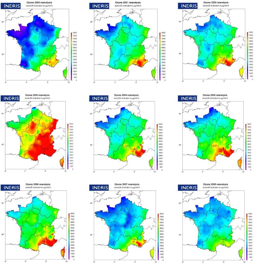
2420                                            E. Real et al.: Historical reconstruction of background air pollution in France

   As a complement to observations (which provide only            again there is no multi-year consistency as these European
partial spatial information), accurate, high-spatial-resolution   maps are produced on an annual basis with gradually im-
and up-to-date air pollution maps are important information       proving methodologies (Marécal et al., 2015). At the global
for assessing air pollution trends and exposure. They should      scale, the Global Burden of Disease also makes available air
provide geographically detailed information on the concen-        pollution exposure maps; a recent update of the methodology
trations of air pollutants over the whole territory. These maps   was presented in (Shaddick et al., 2017), but the resolution is
serve as a basis for informing citizens, designing and strati-    0.1◦ or about 10 km.
fying monitoring networks, supporting policy strategies, and         The purpose of this paper and the associated datasets is
measuring their impact. They are also used to estimate pop-       to present and provide mapped data of O3 , NO2 , PM10 and
ulation exposure to air pollutants, which is essential for epi-   PM2.5 concentrations at high spatial and temporal resolu-
demiological studies.                                             tion and associated regulatory indicators covering the French
   On a European scale, different mapping approaches have         metropolitan territory for the period 2000–2015 (2007–2015
been used to produce maps of pollutant concentrations.            and 2009–2015 for hourly concentrations of PM10 and
These maps can be obtained by modeling using a regional           PM2.5 ). The same kriging technique as in the Prev’air sys-
chemistry transport model (CTM) that simulates the con-           tem is used to combine modeled and observed concentra-
centration of pollutants over Europe. However, these mod-         tions. Hourly concentrations of PM10 , PM2.5 , NO2 and O3
els cannot always be used over the whole of Europe with           are produced and mapped over France, and these hourly data
a high resolution and have some biases and limitations in         are then used to calculate and map European and French air
spatial representativeness. Regression methods (Briggs et al.,    quality standards.
2000; Beelen et al., 2009) are also used at different scales.
These stochastic modeling techniques develop statistical as-      2     Methods
sociations between potential “predictor variables” (land use,
emission sources, topography) and measured pollutant con-         Model outputs and measurements from the permanent moni-
centrations in order to predict concentrations at an unsam-       toring network were combined by external drift kriging (Mal-
pled site. Other frequently used techniques are kriging tech-     herbe and Ung, 2009; Benmerad et al., 2017) to construct
niques. These geostatistical techniques are based on the as-      hourly concentration maps over France for a long period:
sumption that the data are spatially autocorrelated and there-    2000 to 2015. Details on the input data and methods used are
fore take into account the distances between measurements         described in the following paragraphs. From these corrected
and the spatial structure of the variable. Different types of     hourly concentration data, annual regulatory air quality maps
kriging are used to map the concentrations of air pollutants.     are then constructed over France.
Over France, kriging methods combining information from a
regional CTM (CHIMERE; Mailler et al., 2017) and obser-
                                                                  2.1    Monitoring data
vations are produced daily by the Prev’air operational fore-
casting and mapping system for air quality (Rouïl et al.,         Hourly measurements are extracted from validated reference
2009). Since 2003 (for ozone) and 2005 (for PM10 ), the           datasets. For France, observations are extracted from the
concentration maps simulated for the day before in Prev’air       national air quality databases: BDQA (Base de Données de
have been corrected each morning using observations. The          Qualité de l’Air) before 2013 and GEODAIR (https://www.
kriging technique used in Prev’Air has evolved over time,         lcsqa.org/fr/les-donnees-nationales-de-qualite-de-lair,
and PM2.5 and NO2 concentrations are now also corrected           last access: 19 May 2022) after 2013, as well as
for the day before. Today, a kriging of hourly observations       from the Airbase database (https://www.eea.europa.
with CHIMERE as external drift is applied to map NO2 and          eu/themes/air/air-quality/map/airbase,       last    access:
O3 concentrations. Since 2017, for the mapping of PM10            19 May 2022) for other European countries from
and PM2.5 concentrations, the method used is an hourly co-        2000 to 2012 and from air quality e-reporting (https:
kriging of PM10 and PM2.5 data with CHIMERE as external           //www.eea.europa.eu/data-and-maps/data/aqereporting-9,
drift. These choices are the results of successive studies that   last access: 19 May 2022) from 2013 to 2015. All back-
compared different kriging techniques (Malherbe and Ung,          ground monitoring data over the spatial domain are used in
2009, Beauchamp, 2015). A similar methodology was imple-          the kriging procedure except for stations with measurements
mented for an earlier reconstruction of outdoor air pollution     above the 95 percentiles. This includes rural, suburban and
in Europe for the period 1989–2008 in Bentayeb et al. (2014).     urban stations but excludes industrial and traffic stations
There are also ambient air pollution maps produced at Euro-       that are representative of very local concentrations and are
pean scale at 1 km resolution by the European Environment         difficult to reproduce in a national-scale mapping system.
Agency but only for selected annual indicators and without        The number of background monitoring sites for each type of
consistency for multi-year reconstructions (Horálek et al.,       station and for each year is summarize in Table 1.
2012, 2020). The Copernicus Atmosphere Monitoring Ser-               Until 1 January 2007, operational monitoring of PM10
vice has also produced European analyses since 2015, but          and PM2.5 was carried out in France by automatic measur-

Earth Syst. Sci. Data, 14, 2419–2443, 2022                                        https://doi.org/10.5194/essd-14-2419-2022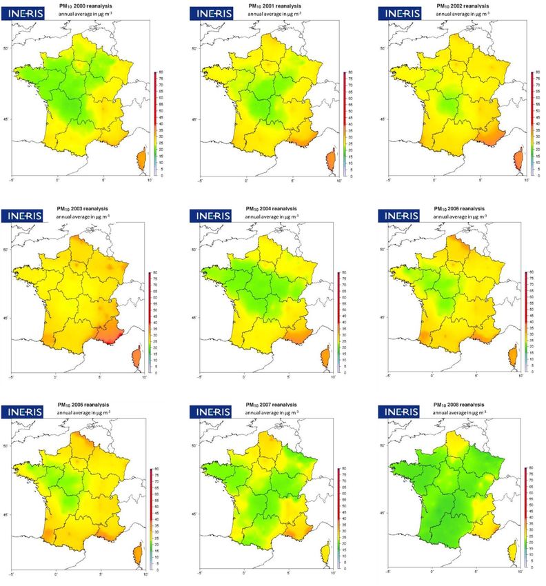
E. Real et al.: Historical reconstruction of background air pollution in France                                                     2421

Table 1. Number of background French monitoring sites for the years 2000 to 2015.

          2000    2001    2002    2003   2004    2005    2006      2007   2008      2009        2010   2011   2012   2013   2014   2015
 O3         284    310     337     362     378    396     404      405      399         385      376    360   347    318    319    331
 NO2        274    290     299     322     337    353     353      350      352         337      334    316   299    284    282    300
 PM10       119    125     171     212     219    238     126      219      252         241      249    245   240    218    173    251
 PM2.5                                                                                   62       69     74    84     89     90    105

ing systems of the TEOM (tapered element oscillating mi-                 For the period 2011 to 2015, year-to-year emissions
crobalance; PM10 , PM2.5 ) or Beta (PM10 ) type. However,             of the main pollutants are taken from the cooperative
compared to the reference method EN 12341 (gravimetry),               program for the monitoring and evaluation of the long-range
these systems underestimate the concentrations of particles.          transmission of air pollutants in Europe (EMEP) avail-
This is a known artifact related to the loss of semi-volatile         able at https://www.ceip.at/webdab-emission-database/
compounds. To correct PM10 concentrations measured be-                emissions-as-used-in-emep-models          (last      access:
fore 2007, a simple approach consists of applying a uni-              19 May 2022). Annual meteorological data were pro-
form correcting factor over France. This method is not suit-          vided by ECMWF with the Integrated Forecasting System
able for correcting hourly or daily concentrations, but it has        (IFS) model with data assimilation.
been shown to work well for annual average PM10 concen-                  For these two datasets, the spatialization of emissions
trations (Malherbe et al., 2017, Bessagnet et al., 2008). The         over France is performed with a 1 km proxy based on the
factor (1.36) is a median value calculated on the PM10 data           national bottom-up emission inventory (available at http:
from “reference” sites (Bessagnet et al., 2008). As a conse-          //emissions-air.developpement-durable.gouv.fr/, last access:
quence, for the period 2000 to 2006, the only PM10 indica-            19 May 2022) which feeds the CHIMERE emission pre-
tor available is the annual average concentration. Concern-           processor described in Mailler et al. (2017). Furthermore,
ing PM2.5 , given the few reference measurements available            Denier van der Gon et al. (2015) showed that primary PM
before 2009, the reliability of even annual measurements is           emissions from residential wood burning can be underesti-
low. It was therefore decided to apply the kriging method-            mated by up to a factor of 2–3 over Europe because the emis-
ology only from the year 2009 onwards, which is when the              sions largely lack semi-volatile compounds. To compensate
change in measurement method had become widespread.                   for this underestimation, a country correction factor deter-
                                                                      mined from Denier van der Gon et al. (2015) is applied over
2.2   CHIMERE simulations                                             the whole period.

The CHIMERE chemistry transport model (Couvidat et al.,
2018) is used to estimate air pollution levels for metropoli-
                                                                      2.3    Kriging
tan France with a resolution of about 4 km (0.06◦ × 0.03◦ )
over the years 2000 to 2015. This model has long been im-             Hourly atmospheric concentration fields are estimated by
plemented and assessed in France as the main component                universal kriging, a geostatistical method. Kriging aims to es-
of the national air quality forecasting and monitoring system         timate the value of a random variable (random process which
PREV’AIR (Honoré et al., 2007). Two types of input data are           describes the observations) at locations from the measure-
used to simulate concentrations.                                      ments. Kriging relies on the concept of spatial continuity,
   Prior to 2010, a configuration similar to the one used in the      which implies that measurements that are close to each other
EURODELTA-Trends project (Colette et al., 2017) is used.              will be more similar than distant measurements. In addition,
The methodology of Colette et al. (2017) is used to recon-            kriging requires a good knowledge of the spatial structure
struct the emissions of the main air pollutants (non-methane          of the interpolation domain which is represented by the var-
volatile organic compound (NMVOC), NOx , CO, SO2 , NH3                iogram or co-variogram (second-order properties) of a ran-
and primary PM): the annual emissions of each country, bro-           dom function (Goovaerts, 1997; Wackernagel, 1996; Chiles
ken down by SNAP (Selected Nomenclature for reporting                 and Delfiner, 2012; Lichtenstern, 2013). Kriging involves de-
of Air Pollutants) sectors, are estimated using the GAINS             riving the linear combination of the observations which en-
(Greenhouse gases and Air pollution Interactions and Syner-           sures the minimal estimation variance under a non-bias con-
gies) model (Amann et al., 2011) for the years 2000, 2005                                                                [
                                                                      dition. At a point s0 , the concentration estimate y(s0 ) is given
and 2010 . To derive emissions for intervening years, secto-          by Eq. (1).
rial results for 5-year periods are linearly interpolated. Mete-
orological data are simulated with the Weather Research and                       N
Forecast Model (WRF version 3.3.1; Skamarock et al., 2008)
                                                                                  X
                                                                       \
                                                                      y(s0) =           λi y(si ),                                    (1)
from 2000 to 2010.                                                                i=1

https://doi.org/10.5194/essd-14-2419-2022                                                     Earth Syst. Sci. Data, 14, 2419–2443, 2022
2422                                                E. Real et al.: Historical reconstruction of background air pollution in France

Figure 1. PM10 : statistical indicators calculated using cross-validation technique on daily mean PM10 values measured and estimated over
rural background stations for the years 2007 to 2015. (a) Number of rural stations for each year. (b) Mean bias (black circles), RMSE (colored
rectangles), correlation (grey crosses and the associated dashed lines) and mean observation (horizontal lines).

Figure 2. PM10 : statistical indicators calculated using cross-validation technique on daily mean PM10 values measured and estimated over
URBAN background stations for the years 2007 to 2015. (a) Number of rural stations for each year. (b) Bias (black circles), RMSE (colored
rectangles), correlation (grey crosses and the associated dashed lines) and mean observation (horizontal lines).

where y(si ), i = 1. . .N , are the observed concentrations at           explanatory variables. This kriging technique has been used
sampling locations through the entire domain (unique neigh-              for several years in monitoring air quality systems for spatial
borhood) or within a limited neighborhood of s0 (moving                  interpolation at the regional scale (PREV’AIR; Malherbe and
neighborhood), and λi , i = 1. . .N , are the kriging weights.           Ung, 2009). For y(s0 ), which is the pollutant concentration to
   Among the kriging methods, the universal kriging (espe-               be estimated at a location s0 , the hypothesis is a linear rela-
cially external drift kriging) allows us to consider additional          tion between y(s0 ) and the considered auxiliary variables as
information to make estimates more accurate. This approach               explained by Eqs. (2) and (3).
is based on a linear regression with auxiliary variables and a
                                                                         y(s0 ) = m(s0 ) + ε(s0 ),                                        (2)
spatial correlation of the residuals, and it allows us to com-
bine simultaneously observations and additional information.             m(s0 ) = b0 + b1 x1 (s0 ) + b2 x2 (s0 ) + . . . + bp xp (s0 ),   (3)
The main hypothesis is that the global mean of the random                where m(s0 ) is the drift of the mean, b0 , b1 , . . .bp are the co-
variable is not constant through the domain, and it relies on            efficients of the linear regression, and x0 , x1 , . . .xp are the

Earth Syst. Sci. Data, 14, 2419–2443, 2022                                                 https://doi.org/10.5194/essd-14-2419-2022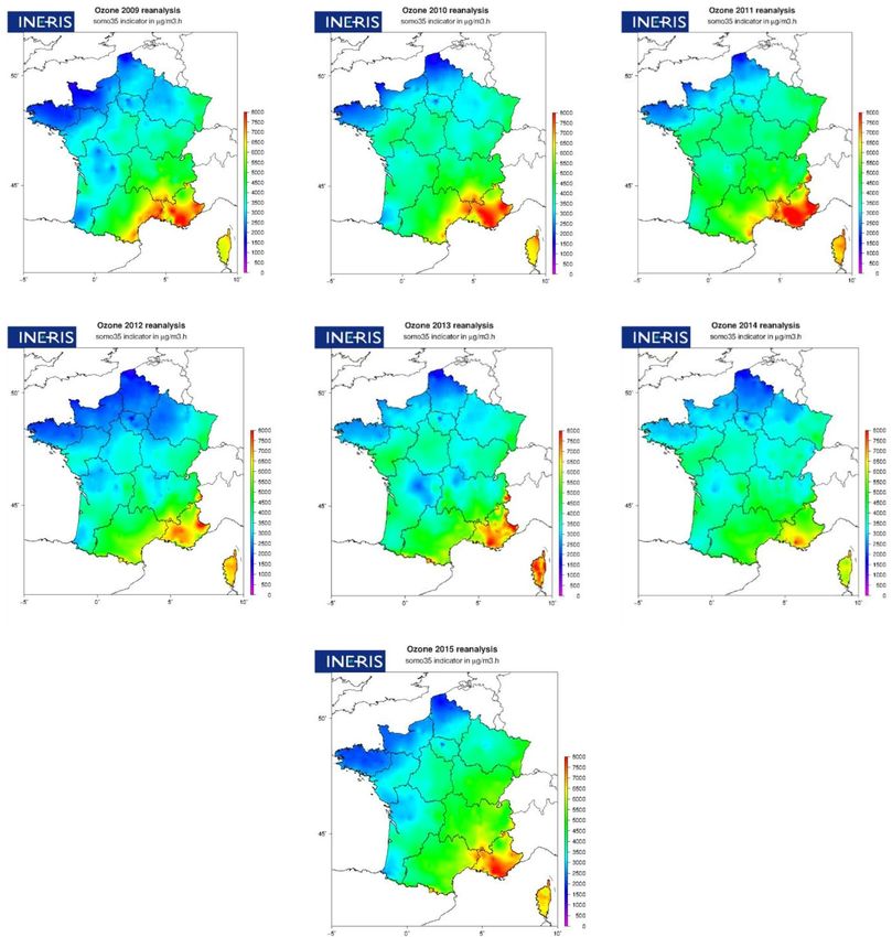
E. Real et al.: Historical reconstruction of background air pollution in France                                                      2423

Figure 3. PM2.5 : statistical indicators calculated using cross-validation technique on daily mean PM2.5 values measured and estimated over
rural background stations for the years 2009 to 2015. (a) Number of rural stations for each year. (b) Bias (black circles), RMSE (colored
rectangles), correlation (grey crosses and the associated dashed lines) and mean observation (horizontal lines).

Figure 4. PM2.5 : statistical indicators calculated using cross-validation technique on daily mean PM2.5 values measured and estimated over
URBAN background stations for the years 2009 to 2015. (a) Number of rural stations for each year. (b) Bias (black circles), RMSE (colored
rectangles), correlation (grey crosses and the associated dashed lines) and mean observation (dotted horizontal lines).

auxiliary variables. ε corresponds to the stationary random             the CHIMERE chemistry transport model. European stations
process which is associated with a semi-variogram. In ad-               located outside the French domain are included in the krig-
dition, the kriging weights must satisfy the drift condition            ing to increase accuracy at the borders. The kriging is per-
described in Eq. 4.                                                     formed using a moving neighborhood as this allows for lo-
                   N                                                    cal adjustment of the relationship between the measurements
                   X
∀xp : xp (s0 ) =         λi xp (si )                           (4)      and CHIMERE. The concentration at each grid point is es-
                   i=1                                                  timated within a window of 80 monitoring sites. This num-
                                                                        ber has been adjusted in previous studies by sensitivity tests
  In this work, kriging is performed with surface monitoring
                                                                        (Benmerad et al., 2017; Beauchamp et al., 2017). In addi-
observations, and the drift is described by the outputs from

https://doi.org/10.5194/essd-14-2419-2022                                               Earth Syst. Sci. Data, 14, 2419–2443, 2022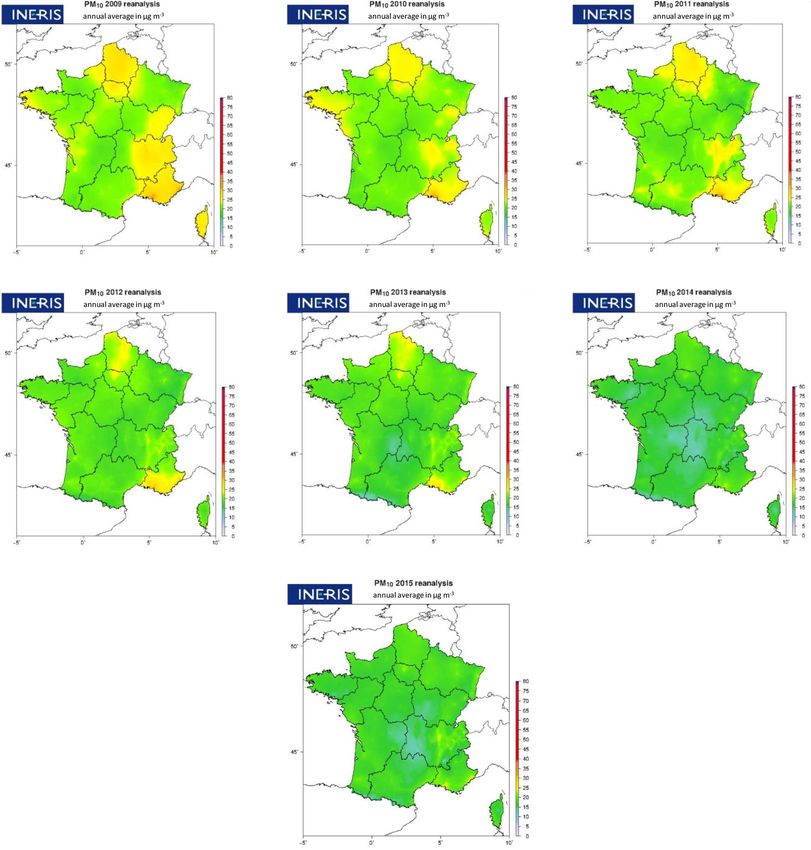
2424                                              E. Real et al.: Historical reconstruction of background air pollution in France

Figure 5. O3 : statistical indicators calculated using cross-validation technique on daily mean O3 values measured and estimated over ru-
ral background stations for the years 2000 to 2015. (a) Number of rural stations for each year. (b) Bias (black circles), RMSE (colored
rectangles), correlation (grey crosses and the associated dashed lines) and mean observation (horizontal lines).

tion, smoothing is applied to avoid discontinuities in the map         residuals (De Fouquet et al., 2007). Co-kriging allows us to
(Beauchamp et al., 2015); the smoothing methodology was                take into account the correlation between PM10 and PM2.5
adapted from Rivoirard and Romary (2011). The final output             and to improve consistency between PM10 and PM2.5 esti-
resolution is the same as for the CHIMERE model: approxi-              mates (Beauchamp et al., 2015). This co-kriging also allows
mately 4 km resolution (0.06◦ × 0.03◦ ).                               the PM2.5 estimate to benefit from the higher density of PM10
   For PM10 (particles with a radius < 10 µm) and PM2.5                monitoring stations.
(particles with a radius < 2.5 µm) a co-kriging with external
drift is applied. Co-kriging is an extension of kriging to the         2.4   Output: regulatory air quality indicators
multivariate case. It allows the estimate of PM10 or PM2.5
concentrations by a linear combination of the two-variable             From the hourly kriged concentrations, several air quality in-
data. The particularity of co-kriging is the use of the cross          dicators (regulatory and used in health impact assessments)
variance or semi-variance between the principal variable and           are calculated and mapped over France. The complete list
the secondary variable. In the case of co-kriging with exter-          and definition of these indicators are given in Table 2.
nal drift, the simple and cross variograms are built based on

Earth Syst. Sci. Data, 14, 2419–2443, 2022                                              https://doi.org/10.5194/essd-14-2419-2022
E. Real et al.: Historical reconstruction of background air pollution in France                                                    2425

Figure 6. O3 : statistical indicators calculated using cross-validation technique on daily mean O3 values measured and estimated over UR-
BAN background stations for the years 2000 to 2015. (a) Number of urban stations for each year. (b) Bias (black circles), RMSE (colored
rectangles), correlation (grey crosses and the associated dashed lines) and mean observation (horizontal lines).

3   Data validation                                                    cations without measurements (provided they are within the
                                                                       area covered by the measurements).
                                                                          It was noticed that the scores are systematically different at
Usually the quality of the estimated concentration maps is as-         rural and urban stations (even though the kriging technique
sessed using statistical indicators that compare observations          used here is not differentiated by the type of station). This
and estimated concentrations at the monitoring stations in             is why the results of the cross-validation are described by
the domain. Here, information of all background stations in            pollutant and differentiated by station type (rural and urban
the domain is already used to produce the maps. Therefore,             types are presented here). Three statistical indicators are cal-
for a fair comparison, the cross-validation method is used.            culated on the basis of the daily average concentration: the
The cross-validation method calculates the quality of the spa-         mean bias, the root mean squared error (RMSE) and the Pear-
tial interpolation for each measurement station point from             son correlation (r 2 ). For each year, they are first calculated
all available information except the selected station point;           for the “left out” station, and then the median values over all
i.e., it retains one data point and then makes a prediction at         stations are calculated.
the spatial location of this point. This procedure is repeated            Leave-one-out validation is a commonly used method in
for all measurement points in the available set, thus allow-           the air quality community (see, for example, ETC reports
ing the quality of the predicted values to be assessed at lo-          on air quality mapping (Horálek et al. 2017)) which is

https://doi.org/10.5194/essd-14-2419-2022                                              Earth Syst. Sci. Data, 14, 2419–2443, 2022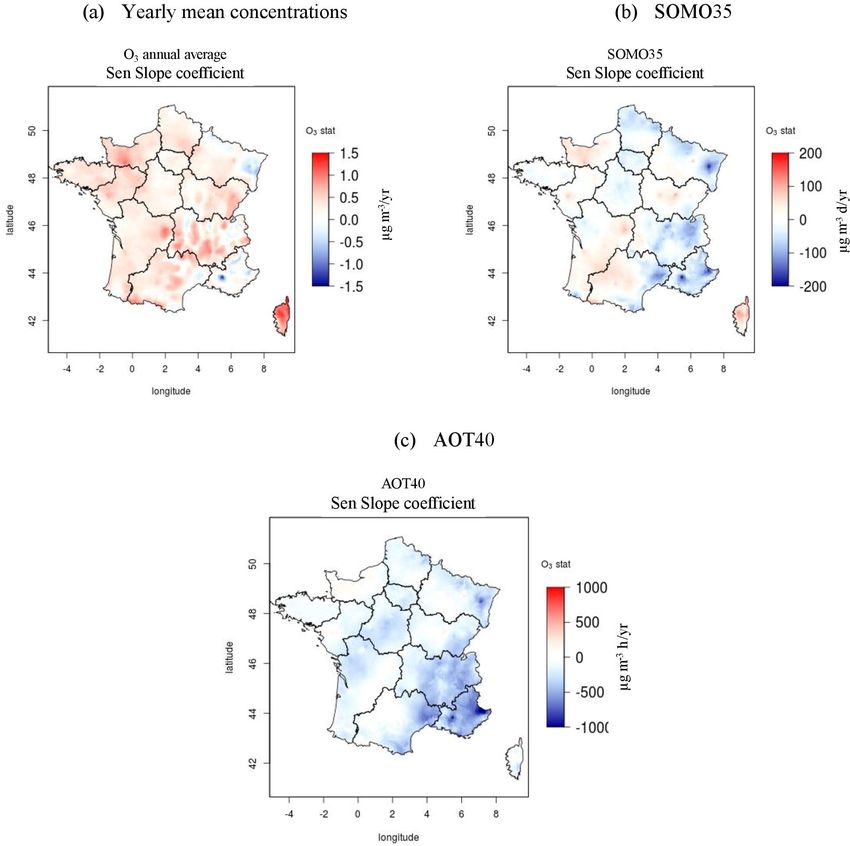
2426                                                                         E. Real et al.: Historical reconstruction of background air pollution in France

Table 2. Yearly regulatory air quality indicators from EU legislation or French legislation and usual indicators.

   ID                           Pollutant      Statistics                                                 Threshold                                         Threshold origin             Target to
                                                                                                                                                                                         protect
   NO2_avgannual                NO2            Yearly average                                             40 µg m−3                                         Limit value (EU)             Human health
   O3_avgannual                 O3             Yearly average
   O3_AOT40                     O3             AOT40∗ from May to July                                    6000 µg m−3                                       Long-term                    Vegetation
                                                                                                                                                            objective
   O3_AOT40_5years              O3             AOT40∗ from May to July (5-year average)                   18 000 µg m−3                                     Target value (EU)            Vegetation
   O3_SOMO35                    O3             Sum of excess of max daily 8 h averages                                                                      Health impact                Human health
                                               over 35 ppb (= 70 µg m−3 ) calculated for                                                                    assessment
                                               all days in a year; SOMO35 (sum of means
                                               over 35 ppb)
   O3_T120                      O3             Number of days for which the running                                                                         Quality      objective       Human health
                                               average over 8 h exceeds 120 µg m−3                                                                          (EU)
   O3_T120_3years               O3             Number of days for which the running 8 h                   Not to exceed more than 25 d a year               Target value (EU)            Human health
                                               average exceeds 120 µg m−3 (averaged over
                                               3 years)
   O3_T180                      O3             Number of hours exceeding the average                                                                        Recommendation               Human health
                                               value of 180 µg m−3                                                                                          and information
                                                                                                                                                            threshold (France)
   O3_T240                      O3             Number of hours exceeding the average                                                                        Alert threshold              Human health
                                               value of 240 µg m−3                                                                                          (France)
   PM10_avgannual               PM10           Yearly average                                             40 µg m−3                                         Limit value (EU)             Human health
   PM10_t50                     PM10           Number of days exceeding the average                       Not to exceed more than 35 d a year               Limit value (EU)             Human health
                                               value of 50 µg m−3
   PM10_t80                     PM10           Number of days exceeding the average                                                                         Alert threshold              Human health
                                               value of 80 µg m−3                                                                                           (France)
   PM25_avgannual               PM25           Yearly average                                             25 µg m−3                                         Limit value (EU)             Human health
  ∗ AOT40 (expressed in µg m−3 h−1 ) means the sum of differences between hourly concentrations greater than 80 µg m−3 (= 40 ppb or parts per billion) and 80 µg m−3 for a given period using only the 1 h
  values measured daily between 08:00 and 20:00 CET.

presently recommended by FAIRMODE (Janssen and Thu-                                                         stations varies between 1/3 and 1/10. The larger number of
nis, 2020). However, scores derived from the results of the                                                 urban stations allows a better capture of the spatial variability
leave-one-out validation might be influenced by areas where                                                 in concentrations in urban environments.
the density of sampling points is highest. For this reason,                                                    Looking at the evolution of the scores over the years for
during the FAIRMODE project (Riviere et al., 2019), for                                                     rural stations, the number of stations available first increases
which a kriging method similar to the one conducted here                                                    from 2009 to 2012 before decreasing until 2014. In 2015 a
was conducted, a comparison has been performed between                                                      new increase in the number of stations in France begins. For
cross-validation results obtained by the leave-one-out cross-                                               urban stations, the decrease starts earlier (2010), but the evo-
validation and cross-validation results obtained by the 5-                                                  lution is the same. The temporal evolution of the scores gen-
fold cross-validation (cross-validation leaving 20 % of sta-                                                erally follows the number of stations with higher correlations
tions out). Results and related scores were very similar. We                                                and smaller relative mean biases and RMSE when more sta-
therefore decided to continue with the leave-one-out cross-                                                 tions are available. Indeed, the greater the number of stations
validation process for the validation of our kriging results.                                               there are, the more representative the kriging technique will
                                                                                                            be of the real spatial variability. There are exceptions, how-
                                                                                                            ever, like in 2015 for rural stations, which had the second
3.1     PM10                                                                                                worst scores even though that year has the largest number of
The scores show a good representation of the observations by                                                stations.
the kriged data with correlations between 0.77 and 0.86 and
RMSE of about 7 µg m−3 , i.e., between 30 % and 50 % of the                                                 3.2       PM2.5
annual mean PM10 concentration. The mean biases are par-
ticularly low for urban stations with values below −1 %. For                                                There are between a half and a third as many PM2.5 stations
rural stations the average bias is less than + 3 µg m−3 , i.e.,                                             as PM10 stations. However, by using a co-kriging technique,
less than + 15 %. The proportion between rural and urban                                                    the PM2.5 mapping also benefits from PM10 information so

Earth Syst. Sci. Data, 14, 2419–2443, 2022                                                                                             https://doi.org/10.5194/essd-14-2419-2022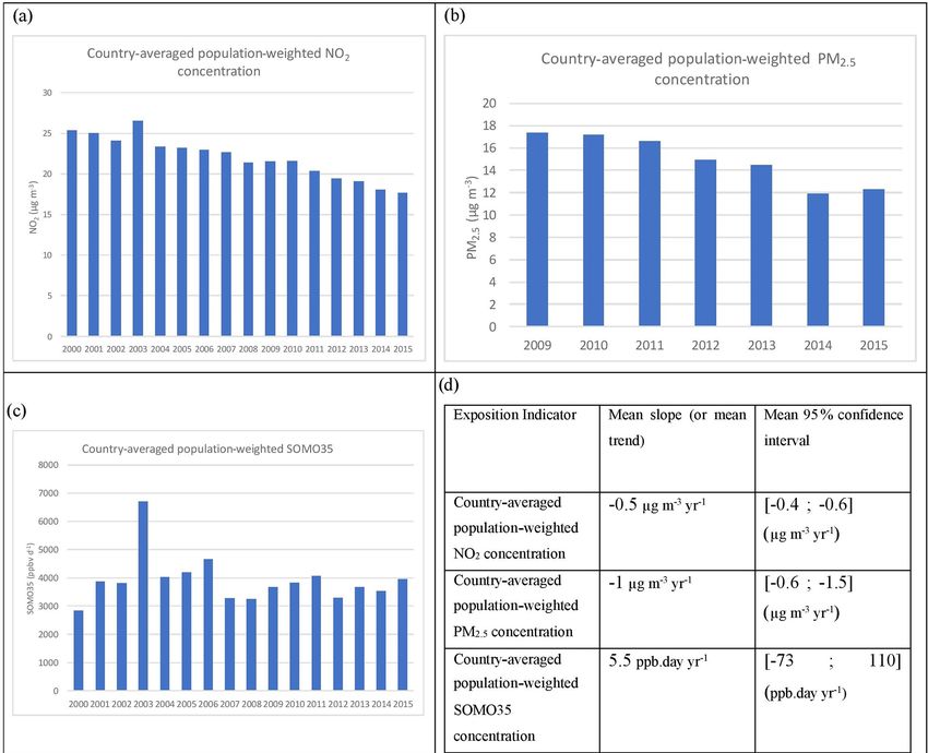
E. Real et al.: Historical reconstruction of background air pollution in France                                                    2427

Figure 7. NO2 : statistical indicators calculated using cross-validation technique on daily mean NO2 values measured and estimated over
rural background stations for the years 2000 to 2015. (a) Number of rural stations for each year. (b) Bias (black circles), RMSE (colored
rectangles), correlation (grey crosses and the associated dashed lines) and mean observation (horizontal lines).

that the correlations, mean bias and RMSE are almost sim-                The correlation is generally higher than 0.8, and the RMSE
ilar to the PM10 scores. The mean biases for rural stations            does not exceed 7 µg m−3 (at most 50 % of the annual mean
do not exceed 20 % of the mean concentrations and are very             concentration).
low for urban stations (between 0 and − 3 %). As for PM10 ,
this bias is systematically positive for rural stations (overes-
timation) and slightly negative over urban stations (underes-          3.3   O3
timation). This is mainly related to the resolution of the data
which smoothes the concentration gradients, giving a unique            The comparison between estimated and observed ozone at
value for each grid (about 4 km horizontal resolution). For ur-        rural stations shows good correlations (0.8 to 0.87), small rel-
ban station, located close to PM2.5 precursor emissions and            ative mean negative biases (−4 % to −8 %) and low RMSE
generally having high concentration values, this smoothing             (around 20 % of the annual mean concentration). Between
effect leads to an underestimation. For rural areas far from           2000 and 2007, the number of rural stations increased, re-
emission precursors, the opposite is observed.                         sulting in improved modeled concentration maps. The small
                                                                       decrease in the number of stations after 2007 does not penal-
                                                                       ize the scores for these years.

https://doi.org/10.5194/essd-14-2419-2022                                              Earth Syst. Sci. Data, 14, 2419–2443, 2022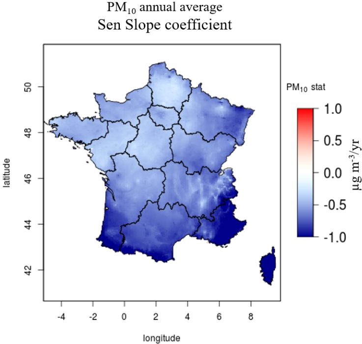
2428                                              E. Real et al.: Historical reconstruction of background air pollution in France

Figure 8. NO2 : statistical indicators calculated using cross-validation technique on daily mean NO2 values measured and estimated over
URBAN background stations for the years 2000 to 2015. (a) Number of urban stations for each year. (b) Bias (black circles), RMSE (colored
rectangles), correlation (grey crosses and the associated dashed lines) and mean observation (horizontal lines).

   The same conclusions can be drawn for the urban ozone               3.4   NO2
scores. The higher number of urban stations even leads to
slightly better scores, with correlations above 0.9 for all years      Rural scores for NO2 are worse for particles and O3 . The cor-
and relative mean positive biases not exceeding 5 %. A sat-            relations are between 0.55 and 0.7, but above all, strong pos-
isfactory RMSE is also obtained for all years with values              itive biases are observed for all years with an overestimation
around 20 % of the annual mean concentration. It can be seen           of the observations of 60 % to 80 %. This also affects RMSE
that the positive and negative biases are reverse with respect         scores that can exceed 100 % of the annual mean concentra-
to the PM scores. Indeed, the highest O3 values are generally          tion. This poor performance can be explained by the strong
observed in rural areas where precursors have had time to              spatial gradients in NO2 concentrations due to its shorter at-
produce O3 and where O3 destruction is lower than in urban             mospheric lifetime than O3 or particles. There are too few
areas. Therefore, the smoothing effect has the opposite effect         rural stations to properly capture this variability in the krig-
to that of PM.                                                         ing technique used here, so the urban stations have too much
                                                                       weight, and the raw model concentrations also overestimate
                                                                       rural concentrations.
                                                                          The urban scores for NO2 are much better than the rural
                                                                       scores. The correlations are around 0.8, the biases do not ex-

Earth Syst. Sci. Data, 14, 2419–2443, 2022                                              https://doi.org/10.5194/essd-14-2419-2022
E. Real et al.: Historical reconstruction of background air pollution in France 2429 Figure 9. https://doi.org/10.5194/essd-14-2419-2022 Earth Syst. Sci. Data, 14, 2419–2443, 2022
2430                                            E. Real et al.: Historical reconstruction of background air pollution in France

Figure 9. PM10 annual mean concentrations from 2000 to 2015. Concentrations are obtained through a combination of regional modeling
and observations.

Earth Syst. Sci. Data, 14, 2419–2443, 2022                                          https://doi.org/10.5194/essd-14-2419-2022
E. Real et al.: Historical reconstruction of background air pollution in France 2431
Table 3. Validation scores for the raw data and the kriged con-
centrations (cross-validation). Annual scores (bias, RMSE and the
Pearson correlation coefficient r 2 ) are calculated over France for all
years and all stations and are averaged.
NO2 O3 PM10 PM2.5
Raw
Bias −3.51 3.46 −8.91 −4.02
RMSE 12.97 17.26 12.63 8.73
r2 0.55 0.73 0.71 0.75
Kriged concentration
Bias −0.51 −0.07 −0.04 −0.15
RMSE 10.41 12.54 7.64 5.83
r2 0.81 0.92 0.85 0.87
cross-validation of their fine-spatial-scale land-use regres-
sion models (also based on Airbase dataset, satellite obser-
Figure 10. Trends in PM10 annual mean concentration. Sen slope vations, dispersion model estimates and land-use variables
coefficient (µg m−3 yr−1 ) calculated over the period 2000–2015. as predictors) used in Europe for the year 2010. Results
from their cross-validation are compared to our own cross-
validation results in Table 4.
ceed −3.5 %, and the RMSE is between 10 and 12 µg m−3 The comparison of performance in these three studies is
(less than 25 % of the annual mean concentration). The high of course limited by the fact that the spatial coverage dif-
number of urban background stations seems satisfactory to fers: in De Hoogh et al. (2018) and Chen et al. (2019), the
allow the kriging technique to correctly reproduce the spa- cross-validation is computed over the whole of Europe. In
tial variability in NO2 in urban background environments. It this study, the performances are assessed over France.
should be noted, however, that traffic stations are not used For all pollutants the spatial correlation (r 2 ) is better in our
in the present analysis (whether as observational data to be study. At the same time, higher RMSEs are also found for our
compared with or included in kriging). study. This may be due to a larger bias, but we also demon-
strated in our paper that the bias was very small, except at ru-
ral NO2 stations. Since the RMSE score also depends on the
3.5 Comparison with other scores
absolute concentrations, the different spatial coverage may
In order to evaluate the added value of the kriging tech- also play a role. The lower RMSE over Europe could be an
nique compared to the raw CHIMERE model simulations, artifact of including areas where absolute concentrations of
the cross-validation scores can be compared to the raw model NO2 , PM2.5 or O3 are lower than over France.
scores. Table 3 shows the scores averaged over all years and The validation scores obtained, as well as the comparison
all observations without distinction of typology. with raw data and with other mapping methods, allow us to
All scores are strongly improved by the kriging method be confident about the validity of the concentrations obtained
of observations with CHIMERE in external drift. However, and their good representativeness of background concentra-
as can be seen in the previous figures, this improvement is tions, in particular in urban areas. A crucial step appears,
more pronounced in urban areas than in rural areas due to the however, when it comes to the representativeness of rural
much larger number of stations in urban areas, which makes NO2 concentrations which are overestimated in our results.
the kriging more representative of these areas.
The cross-validation scores can also be compared with
those obtained in Europe with other mapping methods. Chen 4 Results and discussion
et al. (2019) compared 16 algorithms to develop Europe-wide
spatial models of PM2.5 and NO2 , included linear stepwise After ensuring the validation of the kriged concentration
regression, regularization techniques and machine learning data, yearly indicators, trend over years and human expo-
methods. Those models were developed based on the 2010 sition are calculated. Hourly concentrations fields are pro-
routine monitoring data from the Airbase dataset, satellite duced from 2000 to 2015 for NO2 , O3 and PM10 ; however,
observations, dispersion model estimates and land-use vari- as explained in Sect. 2, for PM10 only annual mean indicator
ables as predictors. De Hoogh et al. (2018) also performed maps are produced before 2007. PM2.5 hourly concentrations
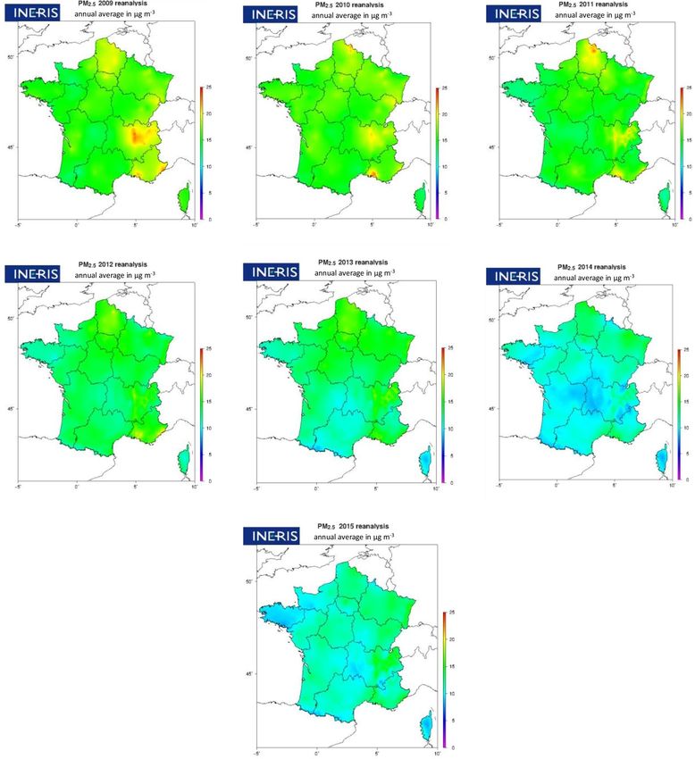
https://doi.org/10.5194/essd-14-2419-2022 Earth Syst. Sci. Data, 14, 2419–2443, 20222432 E. Real et al.: Historical reconstruction of background air pollution in France Figure 11. PM2.5 annual mean concentrations from 2009 to 2015. Concentrations are obtained through a combination (kriging) of regional modeling and observations. Earth Syst. Sci. Data, 14, 2419–2443, 2022 https://doi.org/10.5194/essd-14-2419-2022
E. Real et al.: Historical reconstruction of background air pollution in France                                              2433

                                                                    which the patterns of large inter-regional concentrations are
                                                                    decreasing. The impact of meteorological conditions is also
                                                                    visible through the interannual variability. For example, the
                                                                    2003 heat wave year is associated with higher PM10 levels
                                                                    due to the increased formation of secondary aerosols.
                                                                       Figure 10 shows the mapped trends in annual average
                                                                    PM10 expressed as Sen–Theil regression slope in micro-
                                                                    grams per cubic meter per year and calculated over the period
                                                                    2000–2015.
                                                                       There is a downward trend in PM10 annual mean con-
                                                                    centrations everywhere in France and in particular in the
                                                                    regions with the highest PM10 concentrations at the begin-
                                                                    ning of the period: the south of France (east and west), the
                                                                    Auvergne–Rhône–Alpes region, the east (Grand Est) and
                                                                    the extreme north of France. A country-averaged downward
                                                                    trend in PM10 concentrations of −0.8 µg m−3 per year is es-
                                                                    timated over the period 2000–2015 (spatial average of the
                                                                    trends calculated on each grid point). This trend is statisti-
                                                                    cally significant on average over France with a narrow 95 %
                                                                    confidence interval – [−0.50, −1.09] – that does not include
Figure 12. Trends in PM2.5 annual mean concentration. Sen slope     zero (see Table 5) and applies to almost all grid points (maps
coefficients (µg m−3 yr−1 ) calculated over the period 2009–2015.   of confidence interval not shown here). Taking the year 2000
                                                                    as the base year, this amounts to a 39 % reduction. In a study
                                                                    conducted for France over the period 2000–2010, Malherbe
are calculated for the years 2009 to 2015 due to the limited        et al. (2017) estimated a downward trend that was twice as
number of background stations available before 2009.                small (0.4). This reflects the accelerated decline in concen-
                                                                    trations in France in recent years.
4.1     Concentration maps and trends                                  This significant downward trend is the result of the
                                                                    decrease in primary pollutant emissions over these
All the indicators presented in Sect. 2 are calculated, but the     16 years in response to emission reduction measures.
following sections focus on the annual averaged concentra-          From 2000 to 2015, primary PM10 emissions over
tions of PM10 , PM2.5 , NO2 and O3 , as well as SOMO35 and          France were reduced by 39 %, as well as emissions of
AOT (two indicators associated with O3 ), for which mapped          PM10 precursors such as NOx emissions (−56 %) and
data are presented. These indicators are presented in this pa-      SOx emissions (−87 %) (data calculated by CITEPA
per and available on a Zenodo repository and on an online           (Interprofessional Technical Centre for Studies on Air
map library (see Sect. 5). A total of 34 trend analyses over        Pollution) and extracted from the 2015 French national
the period are performed by calculating the Sen–Theil regres-       air quality report: https://www.statistiques.developpement-
sion slope for each grid point on the domain. To characterize       durable.gouv.fr/sites/default/files/2018-10/datalab-bilan-de-
the significance of these trend slopes, the 95 % confidence         la-qualite-de-l-air-en-france-en-2015-octobre-2016-c.pdf,
interval is calculated. This confidence interval represents the     last access: 19 May 2022).
lower and upper values above or below which there is 95 %
confidence that the trends will occur. The smaller the confi-
                                                                    4.1.2   PM2.5
dence interval is, the more statistically significant the trend
will be. Large confidence intervals are considered as unrep-        The highest PM2.5 values are observed at the beginning of
resentative, especially those containing 0. Trend slopes and        the period and are more concentrated in the main source
confidence intervals are calculated for each grid point in the      regions than PM10 . Significant reductions in annual aver-
domain, and country-averaged values are also given in Ta-           age background concentrations are observed over the years.
ble 5.                                                              The Sen slope coefficients calculated for the annual aver-
                                                                    age PM2.5 (Fig. 12) over the period show negative trends
4.1.1    PM10                                                       over the whole territory and more pronounced ones over the
                                                                    southeast region, the Auvergne–Rhône–Alpes region, north-
Maps of annual average PM10 concentration maps are pre-             ern France and Brittany. A downward trend of −0.87 µg m−3
sented in Fig. 9 for the period 2000–2015. The resolution           per year from a national average is calculated, again with sta-
of the grid (around 4 km) allows us to see patterns such as         tistical significance (95 % interval of [−0.48, −1.41] which
interconnected cities, especially in the latest years during        does not contain zero). Taking 2009 as a reference year, this

https://doi.org/10.5194/essd-14-2419-2022                                           Earth Syst. Sci. Data, 14, 2419–2443, 2022
2434 E. Real et al.: Historical reconstruction of background air pollution in France Figure 13. Earth Syst. Sci. Data, 14, 2419–2443, 2022 https://doi.org/10.5194/essd-14-2419-2022
E. Real et al.: Historical reconstruction of background air pollution in France                                                 2435

Figure 13. SOMO35 indicator for the period 2000 to 2015. Ozone concentrations are obtained through a combination (kriging) of regional
modeling and observations.

https://doi.org/10.5194/essd-14-2419-2022                                            Earth Syst. Sci. Data, 14, 2419–2443, 2022
2436                                            E. Real et al.: Historical reconstruction of background air pollution in France

Figure 14. Trends in annual mean O3 concentrations (in µg m−3 yr−1 ) (a), as well as SOMO35 (in µg m−3 d−1 yr−1 ) (b) and AOT40 (in
µg m−3 h−1 yr−1 ) (c) indicators. Sen slope are calculated over the period 2000–2015.

amounts to a 35 % decrease in 7 years. As for PM10 , this neg-      and AOT40 over the years are shown in Fig. 14 for the pe-
ative trend is associated with the reduction in primary PM2.5       riod 2000–2015.
emissions and in PM2.5 precursor emissions (SOx , NOx and              For the O3 average annual concentration, small posi-
volatile organic compounds (VOCs)).                                 tive trends are found over France. Two exceptions are the
                                                                    southeast (Provence–Alpes–Côte d’Azur, or PACA, region)
                                                                    and the Grand Est region (east of France), i.e., the regions
4.1.3   Ozone                                                       with the highest O3 concentrations, showing negative trends.
                                                                    Averaging over France, this leads to a positive trend of
The SOMO35 indicator shows strong interannual variability.          0.32 µg m−3 yr−1 which corresponds to an increase of 6.5 %
O3 is a photochemical pollutant produced by secondary re-           over 16 years. The same order of magnitude was found for
actions in the presence of NOx , VOCs and sunlight. The hot         the period 2000–2010 by Malherbe et al. (2017). Both neg-
year 2003 is distinguished by a very high SOMO35 over al-           ative (in the south of France) and positive trends are signif-
most the entire territory. For each year, the highest SOMO35        icant according to the mapped 95 % confidence interval (not
is found in southeastern France and to a lesser extent in the       shown). SOMO35 and AOT40 indicators, which are indica-
Alsace region. The trends in SOMO35, annual average O3

Earth Syst. Sci. Data, 14, 2419–2443, 2022                                          https://doi.org/10.5194/essd-14-2419-2022
E. Real et al.: Historical reconstruction of background air pollution in France 2437 Figure 15. https://doi.org/10.5194/essd-14-2419-2022 Earth Syst. Sci. Data, 14, 2419–2443, 2022
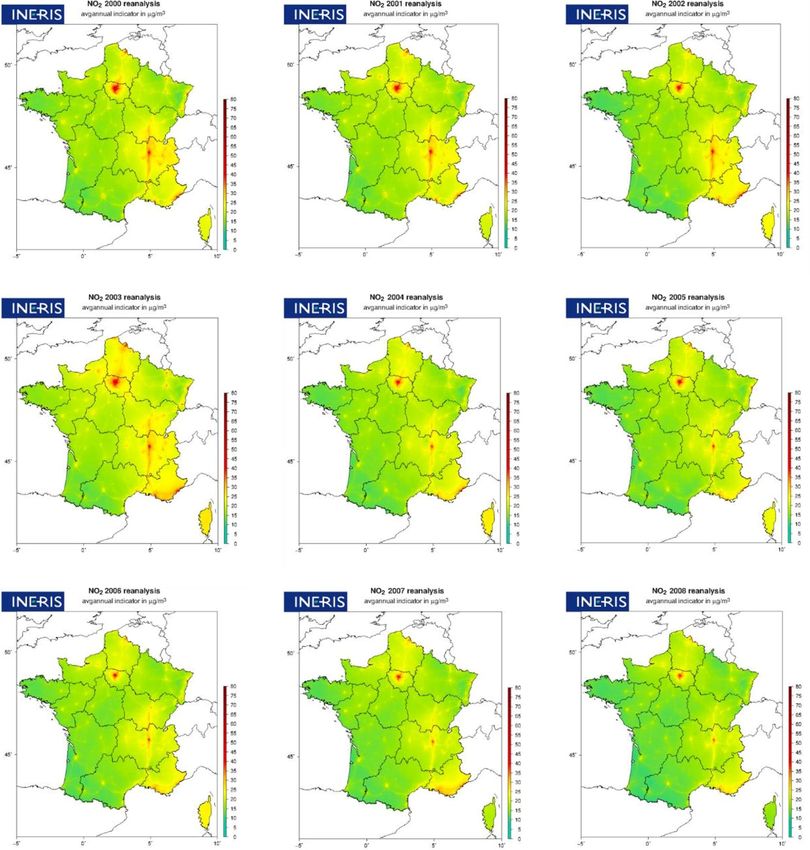
2438                                              E. Real et al.: Historical reconstruction of background air pollution in France

Figure 15. NO2 annual mean concentrations for the period 2000 to 2015. NO2 concentrations are obtained through a combination of regional
modeling and observations.

Earth Syst. Sci. Data, 14, 2419–2443, 2022                                             https://doi.org/10.5194/essd-14-2419-2022
E. Real et al.: Historical reconstruction of background air pollution in France                                                        2439

                                                                          Table 5. Country-averaged slope and its 95 % confidence interval.

                                                                           Indicator             Mean tendency slope            Mean 95 %
                                                                                                   (or mean trend; in   confidence interval
                                                                                                       µg m−3 yr−1 )      (in µg m−3 yr−1 )
                                                                           PM10 – avg annual                   −0.8          [−0.5, −1.09]
                                                                           PM2.5 – avg annual                 −0.87        [−0.48, −1.41]
                                                                           O3 – avg annual                     0.32           [0.005, 0.59]
                                                                           O3 – SOMO35                        −5.52         [−102.7, 76.7]
                                                                           O3 – AOT                           −142             [−641, 315]
                                                                           NO2 – avg annual                   −0.32          [−0.3, −0.63]

                                                                          4.1.4    NO2
                                                                          NO2 is mainly emitted by road transport. All maps show
                                                                          the same pattern, with cities and interconnected major roads
                                                                          showing the highest NO2 concentrations. Trends over the
                                                                          period 2000–2015 are shown in Fig. 15. Decreases in NO2
                                                                          concentrations are observed in both rural and urban areas
                                                                          throughout the country. However, we recall that rural lev-
Figure 16. Trends in yearly mean NO2 concentrations. Sen slope
                                                                          els were found to be overestimated with our approach (see
coefficients (µg m−3 yr−1 ) are calculated over the period 2000–
2015.
                                                                          Sect. 3.4). The decrease is more important when NO2 con-
                                                                          centrations are high. As with PM2.5 , these results highlight
                                                                          the combined benefit of large-scale emission management
                                                                          policies that target emission sectors and locally oriented poli-
Table 4. Validation scores for De Hoogh et al. (2018), Chen et            cies.
al. (2019), and this study. The following scores are calculated by           On average, a significant negative trend of −0.46 µg m−3
cross-validation for the three studies: Pearson correlation coefficient   is calculated over France with a narrow 95 % confidence in-
r 2 , the bias, and the root mean square error (RMSE).                    terval (see Table 3). This downward trend is slightly stronger
                                                                          than that calculated in Malherbe et al. (2017) over the pe-
                         De Hoogh et al.     Chen et al.      This        riod 2000–2010 over France (−0.37 µg m−3 yr−1 ) and corre-
                                (2018)          (2019)       study        sponds to a reduction of about 30 % (taking 2020 as the base
    NO2       r2                     0.57     0.57–0.62      0.81         year).
              RMSE                   9.51         9–9.5     10.41
              Bias                                          −0.51         4.2     Exposure trends
    PM2.5     r2               0.58–0.68      0.48–0.63      0.87         Population-weighted annual average concentrations are good
              RMSE              2.97–3.3         3.1–3.9     5.83         estimates of population exposure as they give more weight to
              Bias                                          −0.15         the air pollution where people mainly live. Here, the country-
    O3        r2                     0.63                    0.92         averaged population-weighted concentrations of NO2 , PM2.5
              RMSE                   6.87                   12.54         and SOMO35, which are the three main indicators used to
              Bias                                          −0.07         calculate health impacts, are calculated for each year from
                                                                          the hourly kriged mapped data over France. For one pollu-
                                                                          tant, it is obtained by adding the result of multiplying the
                                                                          concentration by the population on all the country’s grids
                                                                          and then dividing by the total population of the country.
tors with a threshold value below which concentrations are                The population database used in this study is the LCSQA
not taken into account, show mostly negative trends. How-                 (L’expertise au service de la qualité de l’air) national popu-
ever, according to the value of the mapped 95 % confidence                lation database (Létinois et al., 2014) established for the year
interval (not shown here) on most grid points, the confidence             2015. It is based on detailed files from the French Ministry
interval is wide and contains zero, indicating a lack of signif-          of Finance with information at building level. It is impor-
icance of the calculated trends. These results are consistent             tant to note that the French population used here has not var-
with other European studies (EMEP, 2016; Malherbe et al.,                 ied over the years. The French population increased by about
2017) that show an increase in background concentrations                  10 % between 2000 and 2015. However, if we considered that
and a decrease in O3 peaks.                                               the demographic evolution is homogeneous over the country

https://doi.org/10.5194/essd-14-2419-2022                                                 Earth Syst. Sci. Data, 14, 2419–2443, 2022
2440 E. Real et al.: Historical reconstruction of background air pollution in France
Figure 17. Yearly evolution of the country-averaged population-weighted (a) NO2 concentration, (b) PM2.5 concentration and (c) SOMO35.
Trends and 95 % confidence intervals are calculated (d).
(the urban/rural ratio has only increased by about 2.5 % in SOMO35, anthropic PM2.5 and NO2 (with or without thresh-
France over the same period), the population-weighted con- old depending on the health impact indicator) contributes
centration on national average should be the same whatever to both morbidity and mortality impacts. For example in
the year of the population database. France, they were used in the PREPA (National Air Pollu-
As for the concentrations, a very clear downward trend tant Emissions Reduction Plan) evaluation study for which
is observed for population-weighted NO2 with a trend of about 50 political measures to be implemented in France
−0.5 µg m−3 yr−1 and a narrow 95 % confidence interval: were evaluated and ranked on different criteria, such as air
[−0.4, −0.6], i.e., a reduction of about 30 % in 16 years. A quality impact, health impact and cost–benefit assessment
downward trend of −1 µg m−3 yr−1 is also clearly calculated (Schucht et al., 2018). At constant population evolution, the
for PM2.5 (95 % confidence interval: [−0.6, −1.5]) over the trends are similar between both indicators (total exposure
period 2009–2015, i.e., a reduction of about 31 % in 7 years. and population-weighted average concentration). However,
In contrast, there is no clear trend for the SOMO35 indicator the evolution in population (even if it is homogeneous over
over the period 2000–2015. the territory) has an impact on the total exposure of the pop-
When the abovementioned indicators are multiplied by the ulation. Therefore, we expected a reduced impact on health
total population (to obtain the total exposure, i.e., the sum compared to those on population-weighted concentrations.
of the population-weighted concentrations over a country),
the outcome indicators are those used to calculate the health
5 Data availability
impact assessment based on dose-response functions, as sug-
gested by the WHO review “Health Risks of Air Pollution
Mapped regulatory indicators and exposure data for
in Europe”, described in Holland (2014a, b). Exposure to
all 15 years and the four pollutants described here are
Earth Syst. Sci. Data, 14, 2419–2443, 2022 https://doi.org/10.5194/essd-14-2419-2022E. Real et al.: Historical reconstruction of background air pollution in France 2441
available on a Zenodo repository in the Netcdf format significant. In general, the background O3 level is increas-
(version no. 4) and csv format for data at the munic- ing, mainly due to large-scale pollution, and high (peaks) O3
ipal or regional level. The DOI link for the dataset is levels are decreasing due to reductions in local O3 precursor
https://doi.org/10.5281/zenodo.5043645 (Real et al., 2021). emissions. This results in a positive trend for the annual aver-
It is also available through a web-based map library (https: age O3 concentration over most of France, but a small down-
//www.ineris.fr/fr/recherche-appui/risques-chroniques/ ward trend is also observed in the regions with the highest
mesure-prevision-qualite-air/20-ans-evolution-qualite-air, O3 levels (southeast and east). No significant trend is calcu-
Real et al., 2021). The web-based map library is intended lated for the two O3 indicators detailed here (SOMO35 and
to be updated annually. Those data have been provided AOT40). Population exposure is also calculated over France.
to several research teams with different fields of expertise The average weight of NO2 and PM2.5 in the population of
ranging from epidemiology to environmental economics and the country decreases respectively by 30 % in 16 years and
atmospheric science. Most of this work is still in progress, 31 % in 7 years. No clear trend was found for the population
but other papers on the subject have been submitted or are weight of SOMO35.
being submitted (Favet et al., 2020; Mink, 2022; Cantrell
and Michoud, 2022).
Author contributions. Data kriging, results evaluation by cross-
validation process, and maps and graph production for the paper
6 Conclusions were performed by ER. The CHIMERE modeling concentration
data over the period 2000–2015 were produced by FC. Software de-
velopments for the kriging and cross-validation methods were pro-
A 16-year datasets of mapped air pollution concentrations
vided by AU, LM and AG. The web-based map library used to store
and indicators over France was constructed using a data fu-
and visualize the data was developed by BR. All work has been
sion technique (kriging) that combines measurements from supervised and conceptualized by AC. The manuscript draft was
background surface monitoring stations and modeling from mainly written by ER with contributions from all co-authors.
the regional model CHIMERE. The resulting data are hourly
concentrations at a resolution of about 4 km over France for
the period 2000–2015 (shorter period for PM2.5 and PM10 Competing interests. The contact author has declared that nei-
hourly indicators). ther they nor their co-authors have any competing interests.
The kriging technique implemented combines kriging
with external drift for NO2 and O3 and co-kriging with exter-
nal drift for particulate matter, allowing the PM2.5 estimation Disclaimer. Publisher’s note: Copernicus Publications remains
to benefit from the highest density of PM10 monitoring sta- neutral with regard to jurisdictional claims in published maps and
tions. These datasets have been evaluated over several years institutional affiliations.
using a cross-validation process that takes into account the
incorporation of measurements in the correction process by
retaining a data point before calculating the score. The krig- Acknowledgements. This work was supported by the French
ing technique significantly improves the validation scores, ministry in charge of ecology. Part of the simulations was carried
out in the XENAIR project funded by the ARC Foundation for Can-
especially in urban areas with very low biases and high corre-
cer Research.
lations. However, a crucial point appears concerning the rep-
resentativeness of NO2 concentrations in rural areas which
are overestimated by the model. A new methodology is be- Financial support. This research has been supported by the Min-
ing developed to better map NO2 concentrations in these ru- istère de l’Écologie, du Développement Durable et de l’Énergie
ral areas. It should be noted that the performance increases (grant no. program DRC16).
with the number of measurements taken into account until
a threshold is reached at which the addition of stations no
longer seems to improve performance. This threshold de- Review statement. This paper was edited by Bo Zheng and re-
pends on the pollutant and is higher for pollutants with a viewed by two anonymous referees.
strong spatial gradient (i.e., NO2 which has a shorter life-
time).
The main annual indicators (mean NO2 , PM10 , PM2.5 , O3 ,
SOMO35 and AOT40) are analyzed in this article, and the References
annual trends are calculated. Significant downward trends are
calculated over the whole period for annual average concen- Amann, M., Bertok, I., Borken-Kleefeld, J., Cofala, J., Heyes,
trations of PM10 , PM2.5 and NO2 . They reflect the reduc- C., Höglund-Isaksson, L., Klimont, Z., Nguyen, B., Posch, M.,
tions in precursor emissions that have taken place in Europe Rafaj, P., Sandler, R., Schöpp, W., Wagner, F., and Winiwarter,
since the 1990s. The trends for O3 over the 16 years are less W.: Cost-effective control of air quality and greenhouse gases
https://doi.org/10.5194/essd-14-2419-2022 Earth Syst. Sci. Data, 14, 2419–2443, 2022You can also read