DERIVATION OF FIBER ORIENTATIONS FROM OBLIQUE VIEWS THROUGH HUMAN BRAIN SECTIONS IN 3D-POLARIZED LIGHT IMAGING - JUSER
←
→
Page content transcription
If your browser does not render page correctly, please read the page content below
ORIGINAL RESEARCH
                                                                                                                                       published: 27 September 2018
                                                                                                                                      doi: 10.3389/fnana.2018.00075

                                            Derivation of Fiber Orientations From
                                            Oblique Views Through Human Brain
                                            Sections in 3D-Polarized Light
                                            Imaging
                                            Daniel Schmitz 1*, Sascha E. A. Muenzing 1 , Martin Schober 1 , Nicole Schubert 1 ,
                                            Martina Minnerop 1,2 , Thomas Lippert 3,4 , Katrin Amunts 1,5 and Markus Axer 1
                                            1
                                             Institute of Neuroscience and Medicine-1 (INM-1), Forschungszentrum Jülich, Jülich, Germany, 2 Center for Movement
                                            Disorders and Neuromodulation, Department of Neurology and Institute of Clinical Neuroscience and Medical Psychology,
                                            Medical Faculty, Heinrich-Heine University, Düsseldorf, Germany, 3 Jülich Supercomputing Center, Forschungszentrum Jülich,
                                            Jülich, Germany, 4 Bergische Universität Wuppertal, Wuppertal, Germany, 5 C. and O. Vogt Institute for Brain Research,
                                            Medical Faculty, Heinrich-Heine University Düsseldorf, Düsseldorf, Germany

                                            3D-Polarized Light Imaging (3D-PLI) enables high-resolution three-dimensional mapping
                                            of the nerve fiber architecture in unstained histological brain sections based on the
                                            intrinsic birefringence of myelinated nerve fibers. The interpretation of the measured
                                            birefringent signals comes with conjointly measured information about the local fiber
                                            birefringence strength and the fiber orientation. In this study, we present a novel approach
                                            to disentangle both parameters from each other based on a weighted least squares
                                            routine (ROFL) applied to oblique polarimetric 3D-PLI measurements. This approach was
                                            compared to a previously described analytical method on simulated and experimental
                                            data obtained from a post mortem human brain. Analysis of the simulations revealed
                           Edited by:
                                            in case of ROFL a distinctly increased level of confidence to determine steep and
                         Laurent Petit,
      Centre National de la Recherche       flat fiber orientations with respect to the brain sectioning plane. Based on analysis of
          Scientifique (CNRS), France       histological sections of a human brain dataset, it was demonstrated that ROFL provides
                        Reviewed by:        a coherent characterization of cortical, subcortical, and white matter regions in terms
                            Karla Miller,
 University of Oxford, United Kingdom
                                            of fiber orientation and birefringence strength, within and across sections. Oblique
                     Caroline Magnain,      measurements combined with ROFL analysis opens up new ways to determine physical
               Massachusetts General
                                            brain tissue properties by means of 3D-PLI microscopy.
   Hospital, Harvard Medical School,
                         United States      Keywords: neuroimaging, modeling, 3D-PLI, white matter anatomy, fiber architecture
                  *Correspondence:
                       Daniel Schmitz
              da.schmitz@fz-juelich.de      1. INTRODUCTION
             Received: 07 May 2018          Understanding the human brain’s function and dysfunction requires a thorough knowledge about
         Accepted: 27 August 2018           the brain’s fiber tracts, forming a dense network of connections within, but also between the
      Published: 27 September 2018          different brain regions. Over the last years, several imaging techniques have emerged which are
                             Citation:      capable of resolving anatomical structures with different spatial resolutions. At the millimeter scale,
            Schmitz D, Muenzing SEA,        diffusion MRI is the most prominent one as it is applicable to both in vivo and post mortem brains
Schober M, Schubert N, Minnerop M,          (Basser et al., 1994; Johansen-Berg and Behrens, 2009; Mori and Tournier, 2014). At ultra-high
      Lippert T, Amunts K and Axer M
                                            resolution two-photon microscopy (Laperchia et al., 2013), light-sheet microscopy (Silvestri et al.,
(2018) Derivation of Fiber Orientations
 From Oblique Views Through Human
                                            2012), and electron microscopy (Knott et al., 2008), amongst others, have been exploited to image
  Brain Sections in 3D-Polarized Light      single cells and neurons in 3D space as well as their local connections. Yet these techniques come
    Imaging. Front. Neuroanat. 12:75.       with the cost of excessive measurement time, large amounts of data and limited fields of view (lateral
      doi: 10.3389/fnana.2018.00075         and axial), impeding the study of larger brain volumes so far.

Frontiers in Neuroanatomy | www.frontiersin.org                                   1                                           September 2018 | Volume 12 | Article 75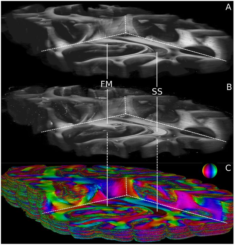
Schmitz et al.                                                                                                 Derivation of Fiber Orientations in 3D-PLI

    3D-Polarized Light Imaging (3D-PLI) (Axer et al., 2011a,b)              data. The examined experimental results represent the first
is a microscopic technique that bridges the gap between large-              analysis of large-scale 3D-reconstructed human brain data in 3D-
scale imaging techniques such as diffusion MRI and ultra-high               PLI. The new approach was introduced in Schmitz et al. (2018)
resolution microscopy. It enables the reconstruction of fiber               for the first time, yet this work represents a vast extension of the
tracts at the meso- and micro-scale from unstained histologial              analysis and results.
sections. Recently, polarization sensitive optical coherence
tomography (PSOCT) has emerged as a promising technique for                 2. MATERIALS AND METHODS
the mapping of fiber bundles with the ability of depth-resolved
scanning of brain blocks (Wang et al., 2011, 2014; Magnain et al.,          2.1. Least Squares Estimation of Fiber
2014). While the signals measured by PSOCT and 3D-PLI both                  Parameters
arise due to the birefringence of brain tissue, their fundamental           2.1.1. 3D-PLI
difference is that PSOCT captures the reflected light instead of            3D-PLI utilizes the birefringence of nerve fibers which is
the transmitted light as 3D-PLI (Caspers and Axer, 2017).                   measured in customized polarimeters. The birefringence
    A pitfall of any histological imaging technique is the extraction       originates from the regular arrangement of lipids in the myelin
of information in the direction perpendicular to the sectioning             sheath resulting in optical anisotropy. This anisotropy causes a
plane, i.e., in the depths of the histological section. While in-           phase shift of incident polarized light passing the brain tissue.
plane fiber orientations can be obtained from texture information           The optical setup as described in Axer et al. (2011b) is depicted
of microscopic images via the structure tensor without the                  in Figure 1: first unpolarized light from an LED array (custom-
need for any biophysical model (Budde and Frank, 2012), little              made design, FZJ-SSQ300-ALK-G, iiM, Germany) passes a
information is directly available about orientations perpendicular          first polarization filter and a quarter-wave retarder mounted
to the sectioning plane. Lately, three-dimensional structure                with a principle axis offset of 45◦ with respect to the polarizer
analysis has been applied to image stacks obtained from                     (Jos. Schneider Optische Werke GmbH, Germany), circularly
light microscopy (Khan et al., 2015) and confocal microscopy                polarizing the light. Then the light interacts with the brain tissue
(Schilling et al., 2016). This comes with several difficulties: the         mounted on a tilting stage. A second polarizer, rotated 90◦ with
prerequisites of a precise 3D-alignment of the image stack as               respect to the first one serves as analyzer. The outgoing light is
well as a coherent contrast over the whole image stack and the              captured with a CCD camera with 14 bit depth (AxioCam HRc,
strong dependency of the obtained orientations on the chosen                Zeiss, Germany), capturing images at a pixel size of 64 × 64µm.
pre-processing pipeline and kernel size of the structure tensor             The filters and the retarder are rotated simultaneously in
(Khan et al., 2015).                                                        steps of ρ = 10◦ , yielding an image series acquired by the
    As an alternative, 3D-PLI enables to determine fiber                    camera.
orientations directly from the measurement data without the                     The effective physical model behind 3D-PLI describes
need for a manual choice of image processing parameters. This               myelinated nerve fibers as negative uniaxial birefringent crystals.
is achieved by taking measurement data from different views                 Assuming ideal optical components, this model yields the
by tilting the brain section and analyzing it with a biophysical            following expression of the light intensity in each pixel during
model (Axer et al., 2011a). Especially, the estimation of the out-          rotation of the filters (Axer et al., 2011a):
of-sectioning-plane orientation (inclination angle) benefits from
the additional information gained by tilting the brain section as                                     IT
                                                                                       I(ρ, ϕ, δ) =      · 1 + sin(2(ρ − ϕ)) · sin δ                 (1)
it is measured conjointly with the fiber density.                                                      2
    Several algorithms for the analysis of the data acquired with
the tiltable specimen stage have been presented so far. The                 with the transmittance I2T , the in-plane orientation ϕ (direction
Markov Random Field algorithm by Kleiner et al. (2012) and                  angle), and the retardation δ. For the retardation the following
the total variation-cased method by Alimi et al. (2017) both                expression is presumed:
resulted in a robust estimation of the inclination sign. While this
                                                                                                            π
solved the inclination sign ambiguity, the absolute inclination                                        δ=     d cos2 (α)                             (2)
was still undetermined. This problem was first solved by Wiese                                              2
et al. (2014) who showed how the tilted measurements can be                 d with the relative thickness d and the out-of-plane orientation α
utilized to extract inclination and fiber density independently             (inclination angle). For readability purposes we denote d as trel
from each other. Their algorithm is based on a discrete                     in contrast to Axer et al. (2011a). The angles are defined in the
Fourier transformation of the different tilting positions (denoted          range ϕ ∈ [0◦ , 180◦ ] and α ∈ [−90◦ , 90◦ ]. d was introduced by
as DFT algorithm). Due to its analytical nature, the DFT                    Axer et al. (2011a) as the combined effect of section thickness ts ,
algorithm is computationally efficient but suffers from noise               birefringence 1n, and illumination wavelength λ:
instability.
    The here presented approach seeks to overcome this noise                                                   ts 1n
instability and provide a more robust separation of fiber density                                        d=4                                         (3)
                                                                                                                  λ
and orientation. Our approach utilizes a weighted least squares
algorithm to process the tilted measurements. It is then compared           The sinusoidal profile is analyzed with a Fourier analysis: the IT is
to the analytical DFT algorithm on synthetic and experimental               given by the average of the profile, the direction angle by its phase

Frontiers in Neuroanatomy | www.frontiersin.org                         2                                      September 2018 | Volume 12 | Article 75
Schmitz et al.                                                                                                                       Derivation of Fiber Orientations in 3D-PLI

                            A                                                               B

 FIGURE 1 | Experimental setup and tilting coordinate system. (A) Experimental setup. ρ denotes the rotation angle of the polarization filters. Red arrows depict
 possibility to tilt the specimen stage. (B) Tilting coordinate system. Light gray: specimen stage in the planar position without tilt, dark gray: tilted specimen stage. ψ,
 tilting direction angle; τ , tilting angle. Image courtesy: N. Gales.

and the retardation sin δ by its relative amplitude (Axer et al.,                         2.1.2. Light Intensity Distribution of the Imaging
2011a). While this analysis enables unambiguous determination                             System
of transmittance, direction angle, and retardation, α and d are                           For an accurate model of the data acquisition, the noise
mapped onto one value, the retardation. Disentanglement of                                level of the imaging system must be taken into account. As
both parameters is a priori not possible, as any combination of d                         the detected signals are light intensities captured by a CCD
and α which fulfills Equation (2) is valid solution. Furthermore,                         camera in our case, the dominant noise sources are shot noise
for d > 1 the outer sin function induces an additional ambiguity.                         during image acquisition and the internal signal processing
Therefore, the separation of d and α is only bijective for d ∈ (0, 1].                    of the camera (Bertolotti, 1974; Goodman, 2000). Here, the
In Axer et al. (2011a) a constant relative thickness which was                            distribution of interest is the distribution of the number of
extracted by statistical approach is assumed. This enables the                            detected photoelectrons during exposure time per pixel. With
calculation of the inclination by inverting Equation (2). While                           increasing photon count the variance of the photon count
this approach offers a good first guess for the inclinations, the                         increases (Goodman, 2000). The dependency of the variance of
assumption of a constant d over the whole section did not take                            the detected photons σ 2 on the number of detected photons as
local differences between distinct brain regions into account.                            the expected value µ can only be determined experimentally.
For example, the cortex contains far less myelinated axons than                           Therefore, 100 samples of the same scene were taken and
dense white matter regions such as the corpus callosum. Also, it                          analyzed pixelwise for the variances and expected values of the
has to be noted that the relative thickness depends on the section                        measured light intensities. The resulting relationship between
thickness which is not precisely known and the birefringence                              variance and expected value is given by σ 2 = 3µ (cf.
which depends on the local amount of myelin (Goethlin, 1913).                             Supplementary Material for details). The multiplicative factor
Therefore, it is clear that the unbiased disentanglement                                  which relates variance and expected value is called gain factor
of both parameters requires additional measurement                                        g (σ 2 = gµ), in our case g = 3. A common way to model
information.                                                                              overdispersed count data is a negative binomial model as it
    A mechanical solution to gain more measurement                                        allows an arbitrary expectation value and variance. In general,
information is a tiltable specimen stage built into the polarimetric                      the occurrence of k under a negative binomial distribution
system, which introduces a pre-defined tilting angle to the nerve                         parameterized by the expected value and variance is given by
fiber orientation relative to the sectioning plane (Axer et al.,
2011a). By this means, polarimetric measurements can be                                                                          µ2   2           k                µ2
                                                                                                                    k−1+

performed from oblique views. Experimentally, this is realized                                                                 σ 2 −µ  σ      −µ           µ  σ 2 −µ
                                                                                                P(k|µ, σ ) =                                                                   (4)
by a two-nested axis system enabling rotations of the specimen                                                             k                 σ2            σ2
around the x- and y-axis by up to 8◦ . In routine 4 tilting
positions are measured: at each position the brain section is                             The probability to observe the light intensity I given the expected
tilted by ±8◦ with respect to one of the axes, denoted as N(orth),                        light intensity µ and the gain factor g can then be expressed as
S(outh), E(ast), and W(est) (see Figure 1). All measurements
taken with a tilted sample are registered on the measurement
                                                                                                                                      µ             I
                                                                                                                           I−1+

without tilt (planar measurement) by a projective linear                                                                             g−1   g     −1               µ
                                                                                                                                                               − g−1
                                                                                                       P(I|µ, g) =                                         g                   (5)
transformation.                                                                                                                  I               g

Frontiers in Neuroanatomy | www.frontiersin.org                                       3                                              September 2018 | Volume 12 | Article 75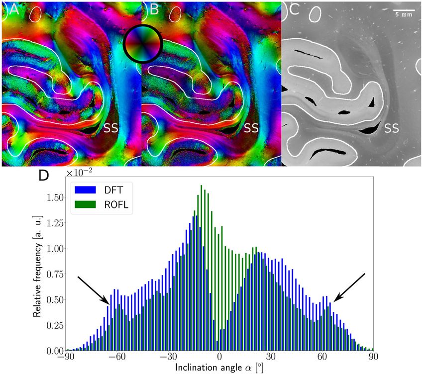
Schmitz et al. Derivation of Fiber Orientations in 3D-PLI
2.1.3. The Tilting Coordinate System which shifts the data into the range [−1, 1]. As the variance
We will use the coordinate system introduced by Kleiner et al. of the light intensities is known as σI2ji = gIji the variance
(2012): it describes the tilting stage by the direction in which of the normalized light intensity can be derived using error
the stage is tilted ψ and the actual tilting angle τ as sketched
propagation as
in Figure 1. For the four tilting directions carried out in the
standard measurement, the tilting directions then are ψ =
0, 90, 180, 270◦ with a tilting angle of τ = 8◦ . With NTilt as the gIji gIji2
σN2 ji = 2
+ 3
(9)
number of tilting positions the tilting directions equidistantly Ij,T NP Ij,T
spanning the space are in general given by ψj = N2π (j − 1), j ∈
Tilt
[1, 2, . . . , NTilt ] with the index j indicating the tilting position. The normalized light intensities fji predicted by the 3D-PLI
The tilted vector rt is obtained by applying the appropriate model are given by inserting Equation (7) into Equation (8):
rotation to the vector in the planar position r: rt = R(ψ, τ )r. The
π
full rotation matrix R(ψ, τ ) is derived by first rotating around
fji (ϕj , αj , dj , ρi ) = sin(2 · (ρi − ϕj )) sin · dj · cos(αj )2 (10)
the z-axis by −ψ, then rotating around the y-axis by τ and then 2
rotating back around the z-axis by ψ (Wiese, 2017):
Fitting f to the normalized light intensities IN can now be
R(ψ, τ ) = Rz (ψ)Ry (τ )Rz (−ψ) formulated as a weighted least squares problem. With the weights
cos(ψ) − sin(ψ) 0
cos(τ ) 0 sin(τ )
cos(ψ) sin(ψ) 0
wij = σN−1
ji
the optimization problem is given by
= sin(ψ) cos(ψ) 0 · 0 1 0 · − sin(ψ) cos(ψ) 0
0 0 1 − sin(τ ) 0 cos(τ ) 0 0 1 NT X
NP
X 2
argmin χ 2 = argmin
cos(τ ) cos(ψ)2 + sin(ψ)2 (cos(τ ) − 1) sin(ψ) cos(ψ) cos(ψ) sin(τ )
fji (ϕj , αj , dj , ρi ) − INji · wji
2 2 ϕ,α,d ϕ,α,d j=0 i=0
= (cos(τ ) − 1) sin(ψ) cos(ψ) cos(τ ) sin(ψ) + cos(ψ) sin(ψ) sin(τ ) .
− cos(ψ) sin(τ ) − sin(ψ) sin(τ ) cos(τ ) (11)
(6) subject to ϕ ∈ [0, π], α ∈ [− π2 , π2 ], d ≥ 0. At this point we do not
restrict the relative thickness to d ≤ 1 as a value of d > 1 could
As stated in Wiese et al. (2014), due to refraction at the brain also occur if the current 3D-PLI model simply does not describe
tissue, the actual tilting angle in the sample is reduced and has to the data well enough. Two issues need to be overcome to solve
be adjusted according to Snell’s law. Assuming a refractive index the optimization problem: the bounded parameter space and a
of n ≈ 1.45 for human tissue based on studies of de Campos Vidal suitable starting point for the local optimization. These issues
et al. (1980), the tilting angle of the light in the tissue is given by resemble the optimization problem of the maximum likelihood
τint ≈ 5.51◦ for a tilt of the tilting stage by τ = 8◦ . algorithm described in Wiese (2017).
A starting point for the direction angle is given by the
2.1.4. Least-Squares Algorithm direction angle derived from the planar measurement ϕ0 . For
We introduce the indices j for the tilting direction (including the inclination α and the relative thickness d, the starting point
0 for the planar measurement) and i for the rotation angle of is determined by brute force minimization. Based on simulation
the polarization filters. Additionaly, we denote the total number studies, a 6 × 6 grid equidistantly spanning the parameter space
of measured tilting stage positions (tilted measurements and ([ϕ0 , αl , dk ], k, l = 1, . . . , 6) was found to result in a promising
the planar measurement) as NT = NTilt + 1 and the number first guess for the subsequent optimization.
of polarizer positions acquired as NP . All measurement data The boundaries of the parameter space could be accounted
accumulates to NT · NP light intensities Iji for each pixel. for by utilizing an optimization algorithm capable of dealing
Application of the Fourier analysis to all measurements as with hard boundaries. Yet, in our case a more elegant solution
described in Axer et al. (2011a) results in NT transmittance values is to exploit the symmetry of the problem. This enables to
Ij,T , NT retardation values | sin δj | and NT direction values ϕj . In reformulate the bounded optimization problem as an unbounded
this notation the intensity curve of a measurement can than be problem. As f (ϕ, α, d) = −f (ϕ, α, −d), it is sufficient to allow all
expressed as relative thicknesses d and take the absolute value of the relative
section thickness d = |d| before calculating the normalized
Ij,T π
1 + sin(2(ρi − ϕj )) sin
Iji (ρi , ϕj , αj , dj ) = dj cos2 (αj ) intensities. For the fiber orientations, it is also possible to allow all
2 2 orientations considering the symmetry of spherical coordinates.
(7)
The unbounded orientation given as (ϕu , αu ) can be transformed
In a first step, the effect of the average light intensity,
back into the standard 3D-PLI parameter space by the following
the transmittance, is eliminated from the fiber orientation
transformations:
determination. Eliminating it from the further process is
necessary as the light experiences additional absorption and π π
1 j ϕu k
refraction effects in a tilted measurement, which cannot be α = αu + mod π − sgn − mod 2 (12)
2 2 2 π
included in the model. Therefore, we define the normalized
light intensity ϕ = ϕu mod π (13)
2Iji Before calculating the normalized light intensities f , these
INji = −1 (8)
Ij,T transformations are used to symmetrize the unbounded
Frontiers in Neuroanatomy | www.frontiersin.org 4 September 2018 | Volume 12 | Article 75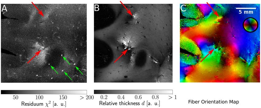
Schmitz et al.                                                                                                        Derivation of Fiber Orientations in 3D-PLI

 Algorithm 1: Pseudocode of the ROFL algorithm                                     (North, South, East, West) by τ = 5.51◦ , the assumed internal
  Data: Maps of ϕ0 , Ij,T , Iji , j ∈ {0, . . . , NT }, i ∈ {0, . . . , NP }       tilting angle for human brain tissue. For each tilting position
  Result: Maps of ϕ, α, d, χ 2                                                     a sinusoidal light intensity profile according to Equation (1)
  for every image pixel do                                                         was calculated. For the transmittance IT 2500 was chosen, as
     // calculate normalized intensities and their standard                        it represents a typical transmittance value for human brain
     deviations                                                                    sections. To mimic the experimentally observed light intensity
     for j = 0 : NT do                                                             distribution, for each calculated light intensity I a noisy light
         for i = 0 : NP do                                                         intensity Inoisy was then computed by drawing one sample from
                      Iji                                                          a negative binomial distribution with expected value given by I
             INji =        −1                                                      and variance 3I: Inoisy ∝ N B(I, 3I).
                     2Ij,T
                                                                                       In a first simulation, the accuracy of the obtained parameters
                 σNji = error prop. of σIj,i , σIj,T to INj,i                      was assessed. As our primary interest here was the validation
       // brute force minimization                                                 of the reconstruction of the inclination and the relative section
       for αl , dk ∈ bruteforce grid do                                            thickness, only one direction angle, ϕ = 45◦ , was simulated.
             2 = χ 2 ϕ , α , d , (I
                                                                                  This direction angle also represents the worst case scenario for
           χl,k         0 l k N00 , σN00 , . . .)
                         2
                                                                                   the four tilting positions as the angle between the orientation
       α0 , d0 = argminχl,k                                                        vector and the rotated orientation vector is maximal for ϕ =
                      α,d
       // optimization                                                             ψ and decreases with |ϕ − ψ|. With respect to the inclination
       Levenberg-Marquardt optimization of χ 2 with initial                        angle, it is sufficient to simulate only positive inclinations as the
       point (ϕ0 , α0 , d0 ) → ϕ, α, d, χ 2                                        inclination sign does not effect the reconstruction precision. As
       transform ϕ, α, d into 3D-PLI parameter space                               ground truth vectors all combinations of the fixed direction angle
                                                                                   45◦ , inclinations α from 0◦ , 1◦ , . . . , 89◦ , 90◦ , and thicknesses
                                                                                   d from 0.01, 0.02, . . . , 0.89, 0.9 were simulated. These fiber
                                                                                   configurations display all different inclination angles for different
orientation into the parameter space. As optimization algorithm                    tissue scenarios characterized by the relative thickness d. For
the Levenberg-Marquardt algorithm was chosen (Levenberg,                           each ground truth vector 100,000 samples of 3D-PLI signals
1944; Marquardt, 1963). In case of convergence to a point outside                  were generated utilizing the beforementioned method to enable a
of the parameter space, the before mentioned transformations                       statistical analysis.
are used to symmetrize the result back into the parameter                              To tests the algorithms against biases in their inclination
space. This newly developped algorithm is denoted as Robust                        estimation, a second dataset of 500,000 samples of orientation
Orientation Fitting via Least Squares (ROFL). A pseudocode is                      vectors uniformly distributed on the unit sphere were computed.
given in Algorithm 1.                                                              From these vectors, a dataset of direction and inclination angles
   For this study, the ROFL algorithm was implemented in                           was derived and used to calculate the noisy sinusoidal light
Python based on the packages NumPy (van der Walt et al., 2011)                     intensity profiles with a relative thickness of d = 0.5.
and SciPy (Jones et al., 2001 ). The necessary computation time
                                                                                   2.2.2. Evaluation
is very high as the optimization has to be carried out in every
                                                                                   The simulated sinusoidal profiles were analyzed with the ROFL
image pixel (about 4 core hours for an image size of ≈ 106 pixels).
                                                                                   algorithm and the DFT algorithm resulting in the reconstructed
Therefore, the algorithm was parallelized pixelwise using mpi4py
                                                                                   vector vr with the parameters (dr , ϕr , αr ). The accuracy of the
(Dalcin et al., 2005) and all calculations were conducted on the
                                                                                   obtained orientation was then measured by the acute angle
JURECA system (Jülich Supercomputing Centre, 2016).
                                                                                   γ between the ground truth vector vg and the reconstructed
2.2. Simulated Data                                                                vector vr :
Monte-Carlo simulations were carried out to test the robustness
                                                                                                           γ = arccos(|vr · vg |)                         (14)
of the presented approach and the DFT algorithm against
measurement noise.                                                                 The acute angle respects the symmetry of the problem: as the
                                                                                   parameter space is bounded to a half sphere, the maximal angle
2.2.1. Generation of Synthetic Data
                                                                                   between two vectors is 90◦ . Therefore, the absolute value of the
Simulations can provide information about two problems.
                                                                                   scalar product is used in Equation (14). For each ground truth
Firstly, the accuracy of the obtained parameters can be compared
                                                                                   vector, the overall reconstruction error is given by the mean
to the synthetic ground truth. Secondly, the algorithms can be
                                                                                   deviation angle hγ i of all 100,000 samples. The reconstruction
tested against biases in their parameter estimation. One sythetic
                                                                                   accuracy of the relative thickness d is evaluated by the absolute
dataset each was created to answer these questions. For both
                                                                                   relative error between the obtained values and the ground truth:
datasets, the generation of synthetic 3D-PLI signals for a specific                        d −d
parameter set is executed in the same way.                                         σd = | rdg g |. The overall error for a fiber configuration is then
   Synthetic signals were generated in a similar manner as in                      again given by the mean relative error of all 100,000 samples hσd i.
Wiese et al. (2014). A ground truth orientation vector vg with                        To assess if the obtained inclinations are biased, inclination
the parameters (dg , ϕg , αg ) was rotated into four tilting positions             angles were reconstructed from the second synthetic dataset. The

Frontiers in Neuroanatomy | www.frontiersin.org                                5                                      September 2018 | Volume 12 | Article 75
Schmitz et al.                                                                                              Derivation of Fiber Orientations in 3D-PLI

resulting inclination angle histograms were then compared to the           computed by the nonlinear image registration. Pixel values
ground truth inclination histogram.                                        were linearly interpolated. The reorientation can result in
                                                                           orientations lying outside of the parameter space, therefore the
2.3. Experimental Data                                                     same mapping as in ROFL (see Equation 13) was applied after
To test and compare the DFT and the ROFL algorithm on                      the reorientation.
experimental data, a series of coronal sections of a right human
hemisphere was investigated. The post mortem human tissue                  2.3.3. Validation
sample used for this study was acquired in accordance with                 Traditional anatomical studies have described the fiber pathways
the local ethic committee of our partner university at the                 globally and without considering differences between brains.
Heinrich Heine University Düsseldorf. As confirmed by the ethic            At the level of detail presented in this study with a voxel
committee, postmortem human brain studies do not need any                  size of 64 × 64 × 70µm3 , the inter-subject variability in
additional approval, if a written informed consent of the subject          the fine structure of fiber orientations becomes much more
is available. For the research carried out here, this consent is           relevant. Therefore, the resulting fiber orientations cannot
available.                                                                 easily be compared to anatomical atlases. A complementary
                                                                           measurement at the same resolution enabling a comparison
2.3.1. Data Acquisition                                                    is not available either. Additionally, a phantom for 3D-PLI
The examined brain was removed within 24 h after the                       has not been developed yet, impeding the possibility of a
donor’s death. The right hemisphere was fixed in 4% buffered               measurement with a known ground truth. Therefore, we chose
formaldehyde solution for 15 days to prevent tissue degeneration.          to validate the resulting orientations based on their coherence
After immersion in a 20% solution of glycerin with Dimethyl                across the whole volume and their alignment to anatomical
sulfoxide (DMSO) for cryoprotection the brain was frozen at a              boundaries, for example, within the sagittal stratum. The results
temperature of −80◦ C. The coronal cutting plane was decided               of both algorithms were furthermore compared from a statistical
to be orthogonal to a line connecting the anterior and posterior           point of view by the difference between the predicted and
commissures. Before sectioning, the frontal lobe was cut off to            measured light intensities measured by the sum of the squared
create a stable cutting platform. The sectioning resulted in 843           residuals.
sections of 70 µm thickness (Polycut CM 3500, Leica, Germany).
Before cutting an image of the cutting surface (blockface image)           3. RESULTS
was taken for each section. Each section was then mounted on
a glass slide, immersed in a 20% solution of glycerin to avoid             3.1. Simulation
dehydration and sealed by a coverslip. All sections were measured          3.1.1. Accuracy Evaluation
with the mentioned setup with the standard measurement                     The simulation results of the first simulated dataset are depicted
protocol of the planar measurement and four tilting positions.             in Figure 2: The plots show the orientation reconstruction error
                                                                           and the relative reconstruction error of the relative thickness of
2.3.2. Data Analysis                                                       both algorithms as a function of inclination angle α and relative
After an intensity based calibration as described in Dammers               thickness d.
et al. (2010) the Fourier analysis was utilized to obtain the
standard 3D-PLI modalities transmittance, retardation and                  3.1.1.1. Orientation reconstruction
direction. Then the ROFL algorithm was used to extract maps of             The orientation reconstruction accuracy of the DFT is valley
the direction and inclination angles, the relative section thickness       shaped with respect to the inclination angle and becomes
d and the residuum χ 2 . As a comparison, the DFT algorithm was            minimal for an inclination angle of α ≈ 60◦ . From this minimum
applied to determine the inclination angle and relative section            the orientation reconstruction error increases slightly for flat
thickness. Also, the residuum was calculated for the parameters            fibers. The most challenging orientations to analyze are very
obtained by DFT.                                                           steep fibers with respect to the sectioning plane: for these, the
   After the sectionwise analysis, the 3D-reconstruction of the            orientations predicted by the DFT algorithm differ strongly from
measured sections requires a multi-step registration to retain the         the ground truth. Even for relative thicknesses of d > 0.2 an
3D volume of the measured brain. Here the blockface volume                 average reconstruction error of hγ i ≈ 22◦ occurs for α > 80◦ .
generated by aligning the blockface images to a 3D volume serves           With decreasing relative thickness d the reconstruction accuracy
as a reference for the registration of the histological sections           also decreases: for d < 0.05, the obtained orientations are
(Schober et al., 2015). In a first step, the histological sections         basically random.
are registered onto their corresponding blockface images via                  In contrast, the orientation reconstruction error for the ROFL
an affine transformation utilizing in-house developed software             algorithm does not take the form of a valley: for all section
based on the software packages ITK (Yoo et al., 2002) and                  thicknesses d > 0.06, the error is minimal for in-plane fibers with
elastix (Klein et al., 2009). Then non-linear registration using           α = 0◦ and increases with the inclination angle. For very steep
the ANTs toolkit (Avants et al., 2011) was performed. Finally,             fibers of α > 80◦ , the error increases to γ ≈ 12◦ on average.
the scalar modalities were spatially transformed using the                 As before, the reconstruction error increases with decreasing
obtained deformation fields. The direction angles were rotated             relative thickness d. In a direct comparison, the orientation
according to the pixelwise rotations induced by the deformation            reconstruction error achieved by the ROFL algorithm is lower

Frontiers in Neuroanatomy | www.frontiersin.org                        6                                    September 2018 | Volume 12 | Article 75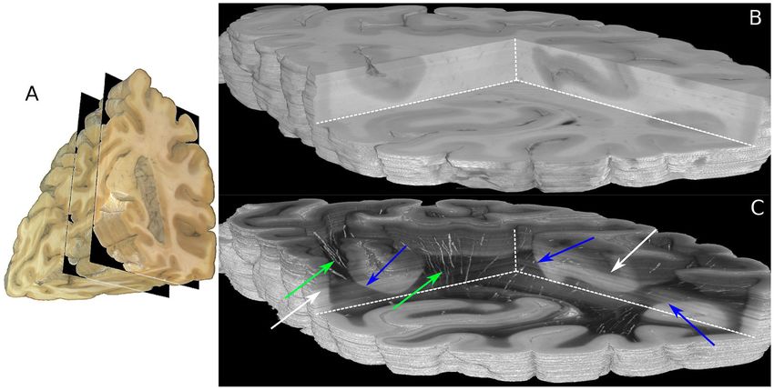
Schmitz et al.                                                                                                                          Derivation of Fiber Orientations in 3D-PLI

 FIGURE 2 | Simulation results. (Left) ROFL algorithm, (Right) DFT algorithm. (Top) Orientation reconstruction error hγ i as a function of relative thickness d and
 inclination angle α. For illustration purposes the z-axis is clipped at 30◦ . (Bottom) relative reconstruction error of the relative thickness hσd i as a function of relative
 thickness d and inclination angle α. For illustration purposes the z-axis is limited to [0, 1].

than the orientation reconstruction error achieved by the DFT                                3.1.2. Inclination Bias Evaluation
algorithm for all configurations. The minimal error for the ROFL                             As the orientation vectors were distributed uniformly on a
algorithm is given by hγ i = 1◦ , compared to hγ i = 1.6◦ for                                sphere, the frequency of the ground truth inclinations is
the DFT algorithm. For d ∈ [0.2, 0.9] and α ∈ [0◦ , 80◦ ], the                               proportional to the circumference of the cross section of
orientation reconstruction accuracy achieved by the algorithms                               the sphere at the respective height corresponding to a given
are on average 2◦ for ROFL and 4.5◦ for DFT with maximal values                              inclination. In our definition of the inclination angle as α ∈
of 9.5◦ for ROFL and 18.8◦ for DFT.                                                          [− π2 , π2 ], the circumference of the cross section of the unit
                                                                                             sphere at a respective inclination is proportional to cos(α). In
3.1.1.2. Reconstruction of the relative section thickness                                    consequence, the inclination frequency p(α) is expected to be
Similar to the the orientation reconstruction error, the relative                            proportional to cos(α): p(α) ∝ cos(α).
reconstruction error hσd i of the relative thickness d increases                                The inclination histograms obtained from the simulated
with the inclination angle. Here, the errors obtained from the                               dataset of uniformly distributed orientation vectors are depicted
DFT algorithm do not assume the shape of a valley: besides a                                 in Figure 3. The histogram of the ground truth inclinations does
noise instability for very high relative thicknesses d > 0.8 the                             indeed follow the expected cos(α) proportionality as can be seen
error increases with the inclination and increases with decreasing                           from the a · cos(α) curve fit with proportionality factor a in cyan.
relative thickness d. The relative reconstruction error of the                               The proposed ROFL approach achieves a high agreement with
ROFL algorithm assumes the same shape but is lower: on average,                              the ground truth inclination. On the other hand, the histogram
the relative thickness of fibers with d ∈ [0.2, 0.9] and α ∈                                 of the inclinations computed by the DFT algorithm reveals a
[20◦ , 90◦ ] is determined with an error of 5% compared to 10% for                           severe lack of in-plane inclinations. Especially orientations with
the DFT algorithm. The most challenging fiber configurations to                              α = 0◦ which are the most probable orientations are barely
reconstruct are again very low relative thicknesses and very steep                           computed at all. Instead of an increasing density toward 0◦ , the
fibers: for d < 0.1 and α < 16◦ , the relative error amounts to                              histogram displays two symmetric peaks left and right of 0◦
hσd i > 1 for both algorithms. For very steep fibers, the error                              indicated by black arrows which are not present in the ground
observed in the results of the DFT algorithm increases to up to                              truth. Another observation lies in the frequency of very steep
80%. The ROFL algorithm achieves a lower error in this case,                                 fibers with respect to the sectioning plane: for |α| > 80◦ , the
yet the best case for d = 0.9 still expresses a relative error of                            frequency of DFT inclinations decreases moderately as indicated
hσ i ≈ 42%.                                                                                  by blue arrows.

Frontiers in Neuroanatomy | www.frontiersin.org                                          7                                              September 2018 | Volume 12 | Article 75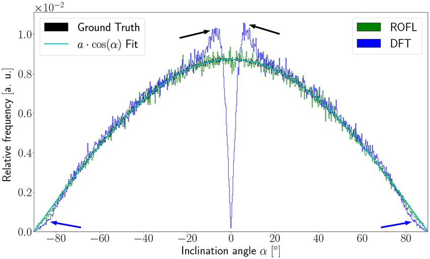
Schmitz et al.                                                                                                                     Derivation of Fiber Orientations in 3D-PLI

 FIGURE 3 | Inclination histograms for uniformly distributed orientations obtained from ROFL and DFT algorithms and ground truth. The magenta line depicts a fit
 curve to the ground truth inclination histogram. Fit result: a = 0.0087. The black arrows highlight peaks for in-plane orientations, the blue arrows point out differences
 between the DFT histogram and the ground truth for out-of-plane orientations. Bin width: 0.25◦ .

3.2. Experimental Data                                                                   perpendicular to the sectioning plane according to the fiber
To demonstrate the working principle of the ROFL algorithm                               orientation map shown in Figure 6C. The forceps major (FM)
by means of experimental data, one pixel of the stratum                                  and the stratum sagittale (SS) were worked out as prominent
sagittale highlighted in Figure 4A was chosen. The obtained                              examples for such tracts (cf. Figure 6). Ultimately, the obtained
measurement data from the planar and two tilted measurements                             fiber orientations (Figure 6), in particular in deep white matter
after calibration and coregistration are plotted in Figure 4B.                           structures appeared coherent across neighboring sections. Fiber
Figure 4C then shows the normalized light intensities and their                          tracts and pathways were clearly distinguishable from each other
best fit curves according to the polarimetric model as predicted                         and could be traced through the reconstructed volume.
by ROFL.
   The boundaries of the investigated 230 coronal sections                               3.2.1. Comparison of ROFL and DFT Algorithms
are illustrated in the view of the blockface volume shown in                             Major differences between the ROFL algorithm and the DFT
Figure 5A (Schober et al., 2015; Wiese, 2017). A comparison                              algorithm were particularly observed for two cases: low relative
of the reconstructed histological sections and the corresponding                         section thickness and very steep fibers with respect to the
part of the blockface volume is depicted in Figures 5B,C utilizing                       sectioning plane. Therefore, the vector fields of two regions
the clipping box view technique implemented in the PLIVIS tool                           were investigated more closely: the stratum sagittale which is
(Schubert et al., 2016, 2018). As the blockface images capture                           expected to run perpendicular to the sectioning plane and a
the reflected light during brain sectioning and the transmittance                        region at the boundary of white and gray matter. The vector
image the transmitted light, they appear inverted to each other.                         fields underlaid with the retardation maps are shown in Figure 7.
As the time between section mounting and measurement was                                 The plotted two-dimensional, colored lines are representations
not constant for all sections, the transmittance differs over                            of the projections of three-dimensional fiber orientation vectors
the volume as indicated by the white arrows in Figure 5C.                                into the respective plane, color-coded by the 3D orientation.
The reconstruction precision is demonstrated by the smooth                               The region of interest at the transition zones of white and gray
reconstruction at the white matter/gray matter transition zones,                         matter shown in Figure 7A. Both vector fields are very similar,
but also by the fine-grained blood vessel structures highlighted in                      but the ROFL algorithm results in less inclined orientations
green in Figure 5C.                                                                      than the DFT approach. As the plotted vectors represent the
   Volumetric views of 3D-PLI modalities are shown in Figure 6.                          projection of the three-dimensional fiber orientation vectors into
For clarity, the view is the same as in Figure 5. The modalities                         the respective plane, longer vectors imply flatter fibers with
retardation | sin δ| (cf. Figure 6A) and relative section thickness                      respect to the respective plane which is the case here. The
d (cf. Figure 6B) revealed a strong agreement in most brain                              vector field in Figure 7B shows the xz plane perpendicular to the
regions of the reconstructed volume. Differences, however, were                          coronal sectioning plane to highlight the robust reconstruction
observed in particular for white matter fiber tracts characterized                       of the stratum sagittale. Minor differences are visible at the
by low retardation values. Those tracts took courses (close to)                          boundary of the stratum sagittale but overall both algorithms

Frontiers in Neuroanatomy | www.frontiersin.org                                      8                                             September 2018 | Volume 12 | Article 75
Schmitz et al. Derivation of Fiber Orientations in 3D-PLI
A
B C
FIGURE 4 | Working principle of the ROFL algorithm demonstrated for a single pixel. (A) Transmittance map. The red circle points out the position of the analyzed
pixel. (B) Measured light intensities of the planar measurement and tilted measurements to west and east after calibration and registration onto the planar
measurement. (C) Normalized light intensities of the planar measurement and tilted measurements to west and east. The dashed lines depict their best fit curves
according to the ROFL algorithm. Fit result: ϕ = 101◦ , α = −60◦ , d = 0.5, R2 = 0.97.
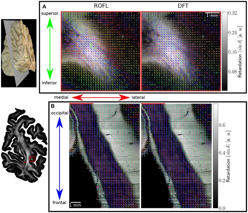
FIGURE 5 | Reconstructed 3D-PLI volumes. (A) Full blockface volume with black planes representing the boundaries of the analyzed sections shown in (B,C).
(B) Partial blockface volume of the histologically analyzed and reconstructed sections. (C) Transmittance volume reconstructed from the histological sections. The
green arrows highlight reconstructed blood vessel structures. Note, for the reasons of clarity only vessels with very strong birefringence signals are shown here. The
blue arrows indicate white/gray matter transition zones. Note that brightnesses variations pointed out by white arrows occur due to differing times between mounting
of the section on the glass slide and the 3D-PLI measurement.
agreed well. As on simulated data the inclination histograms inclination histograms obtained from experimental data were
exposed a distinct lacking of in-plane fiber orientations with also investigated. For this purpose one region of interest from the
respect to the sectioning plane for the DFT algorithm, the white matter of one section was examined. The fiber orientation
Frontiers in Neuroanatomy | www.frontiersin.org 9 September 2018 | Volume 12 | Article 75Schmitz et al. Derivation of Fiber Orientations in 3D-PLI FIGURE 6 | Reconstructed 3D-PLI modalities. (A) Retardation volume, (B) Relative section thickness volume computed by the ROFL algorithm and denoised section-wise with a median filter of radius 1. (C) Fiber orientation volume computed by the ROFL algorithm. The vector-valued fiber orientations are encoded in colors and indicated by the color sphere. FM, forceps major; SS, stratum sagittale. maps (FOMs) resulting from ROFL and DFT are shown in In addition to the potentially biased visual inspection of Figures 8A,B, respectively. A general glance revealed similar the vector fields, an unbiased statistical statement about the orientation values for both algorithms, which holds true for reconstruction accuracy is given by the mean residual: the mean white and gray matter regions. Due to the considerable amount value of the mean residuals of all pixels is 15% lower for the of noise in the fiber orientations in gray matter, only white results of the ROFL algorithm than the results of the DFT matter pixels were considered for the inclination histograms. A algorithm. detailed analysis of the inclination angle histograms of the white matter regions delineated in Figure 8C yielded the following 3.2.2. Agreement of Model and Data observations (cf. Figure 8D): while the frequency of inclination Since the ROFL algorithm performs a least squares fit in all angles drastically decreases from −15◦ to 0◦ and increases again image pixel, the actual sum of residuals χ 2 (as a result of the to 20◦ for the DFT algorithm, this lacking of orientations was not optimization process) was accessible. For the DFT algorithm the observed for the ROFL algorithm. For the regime of high absolute residual map can also be calculated, yet this requires additional inclination angles, both histograms agree: both have peaks for computations which take even longer than the runtime of inclination angles of ≈ ±60◦ (cf. arrows in Figure 8D) which the algorithm itself. Figure 9 shows maps of the residuum χ 2 result from fibers oriented perpendicular to the sectioning plane (Figure 9A), the relative thickness d (Figure 9B) and the fiber in the stratum sagittale (cf. Figures 8A–C). orientation map (Figure 9C) for a selected region of interest. Frontiers in Neuroanatomy | www.frontiersin.org 10 September 2018 | Volume 12 | Article 75
Schmitz et al.                                                                                                                    Derivation of Fiber Orientations in 3D-PLI

 FIGURE 7 | Vectorfields obtained with the ROFL algorithm (left) and the DFT algorithm (right) underlayed with the retardation map. (A) Region of interest at the
 boundary of white and gray matter, indicated by the red rectangle in the retardation map. Every third vector is mapped. (B) Region of interest in the stratum sagittale,
 resliced view of the volume at the position indicated by the red line. Every fifth vector is mapped.

As χ 2 is a measure of the difference between the model and                              4. DISCUSSION AND OUTLOOK
the experimental data, it is expected to increase for artifacts
such as dust particles which rotate with the polarization filters.                       We introduced the least-squares algorithm ROFL for the
Such artifacts were indeed observed in experimental results (cf.                         reconstruction of fiber orientation and the extraction of
Figure 9A, where dust particles are indicated by green arrows).                          the relative section thickness from measurements with a
For one pixel, a dust particle corrupts one of the 18 obtained                           tiltable specimen stage in 3D-Polarized Light Imaging (3D-
values during filter rotation. Still it does not necessarily have                        PLI). This method requires only one additional assumption
a strong effect on the resulting fit values as the corresponding                         besides the polarimetric model: the refractive index of the
relative thicknesses and fiber orientations do not show signs                            brain tissue. This represents a substantial improvement as
of artifacts. The χ 2 measure, however, is sensitive to such                             compared to other histological imaging techniques which
artifacts.                                                                               strongly rely on parameter dependent image processing
   In addition, we found areas of increased residuals (cf.                               pipelines to extract three-dimensional fiber orientations. To our
red arrows in Figure 9) we were able to assign to crossing                               knowledge, no other histological imaging technique is currently
fiber regions. In the fiber orientation map, crossings                                   capable of deriving three-dimensional information from a
stood out as the center of an abrupt change of colors                                    biophysical model. This compensates for the disadvantage of
(Figure 9C). Also, the optimization process resulted in an                               the difficulties accompanying the 3D re-alignment of serial
abrupt change of the relative thickness, even with values of                             high-resolution brain section images as required for 3D-PLI
d > 1 for which the relationship between the retardation                                 anaylsis.
and inclination is not bijective anymore (Figure 9B). Due                                    The working principle of the ROFL algorithm was proven for
to the bad agreement between the model and the data,                                     simulated data for which it resulted in a significant improvement
the residuum finally increased strongly (cf. red arrows in                               of the orientation reconstruction. It was opposed to a previously
Figure 9).                                                                               implemented analytical algorithm based on a discrete Fourier

Frontiers in Neuroanatomy | www.frontiersin.org                                     11                                            September 2018 | Volume 12 | Article 75
Schmitz et al.                                                                                                                   Derivation of Fiber Orientations in 3D-PLI

 FIGURE 8 | 3D-PLI modalities of a representative brain section. (A) Fiber orientation map in the region of the stratum sagittale derived with the ROFL algorithm. (B)
 Fiber orientation map resulting from the DFT algorithm. (C) Transmittance map. The white lines represent a manual delineation of the white/gray matter transition
 zones. SS, stratum sagittale. (D) Histogram of the inclination angles of white matter pixels obtained from DFT and ROFL algorithms. The arrow points out peaks of the
 histogram for steep fibers with respect to the sectioning plane. Bin width: 2◦ .

 FIGURE 9 | Identification of artifacts and fiber crossings. (A) Residuum map χ 2 with green arrows indicating dust particles. (B) Relative thickness map d. (C) Fiber
 Orientation map. Red arrows indicate fiber crossings.

Frontiers in Neuroanatomy | www.frontiersin.org                                    12                                            September 2018 | Volume 12 | Article 75
Schmitz et al.                                                                                               Derivation of Fiber Orientations in 3D-PLI

transformation (DFT). The reconstruction with ROFL became                 angles decreased significantly for in-plane fibers with α ≈ 0◦
more reliable, in particular for low relative section thicknesses.        for the DFT algorithm, the ROFL algorithm was still capable of
The noise instability of the DFT algorithm for very flat fibers           reconstructing the whole spectrum of possible inclinations. The
was already observed by Wiese et al. (2014) and is explainable            same behavior was observed for simulated data, which proves
                                                     sin δ
by the fact that for very flat fibers the gradient ∂ ∂α    becomes        a systematic bias of the DFT algorithm. The ROFL result is
                                          ◦
small (for in-plane fibers with α = 0 it even becomes zero:               also more plausible as for the observed ROI in Figure 8 the
∂ sin δ
  ∂α |α=0
           ◦  = 0). This makes the DFT algorithm prone to                 inclination histogram obtained from ROFL agrees far better with
noise effects in this case. In fact, the simulations proved that          the inclination histogram of uniformly distributed orientations.
the DFT algorithm is not capable of reconstructing in-plane               Still, it has to be noted that fiber orientations in a small ROI of the
orientations. On the contrary, the presented fitting algorithm            brain cannot expected to be perfectly uniformly distributed due
still enabled a reliable reconstruction for in-plane fibers. The          to the convoluted structure of the human brain. The observed
random orientations computed by the DFT algorithm for small               inclination differences between ROFL and DFT are hard to
relative section thicknesses of d < 0.05 were not surprising,             observe based on orientation vectors, as the actual inclination
as for d < 0.05, the maximal possible retardation value is                differences of up to 10◦ for in-plane orientations can barely be
also | sin δ| = 0.05 and the retardation values of the different          distinguished by eye. As the difference between the measured and
tilting positions become almost indistinguishable. In this case,          predicted light intensities according to the 3D-PLI model also
the ROFL algorithm provides a superior reconstruction. In the             decreases significantly for the parameters obtained from ROFL
case of very steep fibers, the ROFL algorithm also outperformed           compared to DFT, ROFL yields more accurate results than DFT
DFT significantly. Still, the reconstruction accuracy decreases           also from a purely statistical perspective.
strongly for very steep fibers also for the ROFL algorithm. This              Furthermore, the ROFL algorithm enables a direct way to
originates from the signal itself: for α = 90◦ , the amplitude of         evaluate the agreement of model and data based on the residuum
the sinusoidal signals are almost zero and the measured signals           map which would otherwise have to be computed additionally.
resemble a constant function with random noise (cf. Dohmen                This kind of map was exploited to identify measurement artifacts
et al., 2015 for a theoretical description of this issue). While          and, even more importantly, crossing fiber regions which were
the reconstruction of out-of-plane fibers remains challenging,            not classifiable by previous 3D-PLI analysis approaches (Axer
orientation vectors with |α| > 80◦ only make up approx. 3% of             et al., 2011a; Kleiner et al., 2012; Wiese et al., 2014). Fiber
all possible orientations. Therefore, we can conclude that ROFL           crossings currently pose the greatest complication for 3D-PLI
accomplishes a very robust orientation reconstruction with an             analysis as partial volume effects are still present in brain tissue
average accuracy of 2◦ for the vast majority of possible fiber            at voxel sizes of 64 × 64 × 70µm3 . A voxel containing fibers
orientations for relative section thicknesses of d > 0.2 on               with different courses (i.e., orientations) will inevitably result in a
synthetic data.                                                           3D-PLI measurement composed of superimposed birefringence
    ROFL was applied to 230 consecutive human brain sections              signals. This might lead to a biased orientation interpretation. To
subjected to 3D-PLI. The results were 3D reconstructed to                 give an example, a voxel comprising crossing out-of-plane and
demonstrate the robustness and reproducibility of our approach.           in-plane fibers, the ROFL algorithm will preferably reconstruct
The obtained modality volumes of retardation, relative section            the orientation which causes a larger signal, in this case the in-
thickness and fiber orientation were characterized by high                plane orientation. To overcome this issue, different strategies are
coherence across the sections. Anatomical structures, such                currently being explored: (i) Modeling of crossing fiber structures
as fiber tracts, white/gray matter borders, vessels could be              and subsequent simulations of tilting measurements utilizing the
reconstructed with high precision. The transmittance volume               simPLI simulation platform introduced by Dohmen et al. (2015).
displayed brightness variations, yet the strength of our approach         By this means the behavior of the ROFL algorithm in case of well-
is that the determination of the fiber orientation and relative           known crossing fiber constellations can be further investigated.
section thickness is independent of the transmittance due to the          (ii) Realizing the idea of oblique imaging for in-plane resolutions
normalization. By eyesight, no major differences were observed            at the micrometer scale. Preliminary measurements of a mouse
in the vector fields resulting from the ROFL and DFT approaches.          section using a prototypic “tilting” polarizing microscope built
In the stratum sagittale, both approaches resulted in very                up at an optical bench (pixel size: 1.3 × 1.3µm) already revealed
similar orientations with very minor differences. The computed            the benefit of smaller voxel sizes.
inclinations were on average α ≈ 65◦ and the computed                         While the obtained parameters show a high coherence across
relative section thicknesses d = 0.6. This combination actually           the volume, no quantitative statement about the reliability
corresponds to the minimum of the orientation reconstruction              of the resulting parameters is possible at this point. Hence,
error of the DFT algorithm obtained from the simulated datasets,          future studies need to investigate the uncertainty of the
which suggests that a strong agreement with the ROFL algorithm            fitted parameters. For Diffusion Tensor Imaging, for example,
can be expected. At the boundary of white and gray matter                 bootstrapping approaches were used to obtain orientation
regions, the ROFL algorithm resulted in less inclined fiber               confidence maps (Jones, 2003; Heim et al., 2004; Whitcher et al.,
orientations than DFT but also only very minor differences were           2008). Especially, the uncertainty of the relative section thickness
observable.                                                               is of interest, as this parameter is as an indicator for myelin and
    The inclination histograms, however, yielded a very important         might even be a reliable measure of the local myelin density. As
finding: whereas, the frequency of the computed inclination               a matter of fact, the relative section thickness is proportional to

Frontiers in Neuroanatomy | www.frontiersin.org                      13                                      September 2018 | Volume 12 | Article 75
Schmitz et al. Derivation of Fiber Orientations in 3D-PLI
the local birefringence 1n which was clearly attributed to the SM and MS: 3D reconstruction, discussion. NS: 3D visualization.
myelin sheath in earlier studies (Goethlin, 1913; Schmidt, 1923; MM: provided the brain sample and anatomical interpretations.
Schmitt and Bear, 1937; de Campos Vidal et al., 1980). Since KA and TL: writing, discussion. MA: study design, discussion,
myelin density information is of outmost interest for the research writing.
of degenerative brain diseases characterized by locally altered
myelination (e.g., multiple sclerosis), future studies will address FUNDING
the correlation between the relative section thickness and myelin
density. This project has received funding from the European Union’s
The improved reconstruction comes at the cost of Horizon 2020 Research and Innovation Programme under Grant
computation time, which increases by a factor of 5,000. Yet, as Agreement No. 7202070 (HBP SGA1) and Grant Agreement No.
processing a single brain section takes about 3 min using four 785907 (HBP SGA2).
compute nodes on JURECA (Jülich Supercomputing Centre,
2016) with the ROFL algorithm in its current implementation, ACKNOWLEDGMENTS
even the computation of whole brains becomes feasible. Still, the
computation time could further be reduced by utilizing GPU We would like to thank Marcus Cremer and Patrick Nysten
ressources (Przybylski et al., 2017). for the preparation of the examined brain sections and
To conclude, the present approach has opened up a new Felix Matuschke for fruitful discussions about the statistical
way to determine physical tissue properties from oblique analysis. We also thank David Gräßel who significantly helped
measurements in microscopic 3D-PLI. Cortical, subcortical, and in identifying anatomical structures. The authors gratefully
white matter regions could be characterized coherently across acknowledge the computing time granted by the JARA-HPC
brain sections in terms of fiber orientation and birefringence Vergabegremium and provided on the JARA-HPC Partition part
strength. This is a prerequisite for subsequent volume-based of the supercomputer JURECA at Forschungszentrum Jülich.
connectivity analysis.
SUPPLEMENTARY MATERIAL
AUTHOR CONTRIBUTIONS
The Supplementary Material for this article can be found
DS: study design, algorithm implementation, simulation, online at: https://www.frontiersin.org/articles/10.3389/fnana.
processing of experimental data, evaluation, writing, discussion. 2018.00075/full#supplementary-material
REFERENCES means of independent component analysis. Neuroimage 49, 1241–1248.
doi: 10.1016/j.neuroimage.2009.08.059
Alimi, A., Pizzolato, M., Fick, R. H. J., and Deriche, R. (2017). “Solving de Campos Vidal, B., Mello, M. L., Caseiro-Filho, A. C., and Godo, C. (1980).
the inclination sign ambiguity in three dimensional polarized light Anisotropic properties of the myelin sheath. Acta Histochem. 66, 32–39.
imaging with a pde-based method,” in 2017 IEEE 14th International doi: 10.1016/S0065-1281(80)80079-1
Symposium on Biomedical Imaging (ISBI 2017) (Melbourne, VIC), Dohmen, M., Menzel, M., Wiese, H., Reckfort, J., Hanke, F., Pietrzyk,
737–740. U., et al. (2015). Understanding fiber mixture by simulation in
Avants, B. B., Tustison, N. J., Song, G., Cook, P. A., Klein, A., and 3D polarized light imaging. Neuroimage 111(Suppl. C), 464–475.
Gee, J. C. (2011). A reproducible evaluation of ants similarity metric doi: 10.1016/j.neuroimage.2015.02.020
performance in brain image registration. Neuroimage 54, 2033–2044. Goethlin, G. F. (1913). Die Doppelbrechenden Eigenschaften des Nervengewebes.
doi: 10.1016/j.neuroimage.2010.09.025 Stockholm: Kungliga Svenska Vetenskapsakademiens Handlingar, 51.
Axer, M., Amunts, K., Grässel, D., Palm, C., Dammers, J., Axer, H., et Goodman, J. (2000). Statistical Optics. New York, NY: Wiley.
al. (2011a). A novel approach to the human connectome: ultra-high Heim, S., Hahn, K., Sämann, P. G., Fahrmeir, L., and Auer, D. P. (2004). Assessing
resolution mapping of fiber tracts in the brain. Neuroimage 54, 1091–1101. DTI data quality using bootstrap analysis. Magn. Reson. Med. 52, 582–589.
doi: 10.1016/j.neuroimage.2010.08.075 doi: 10.1002/mrm.20169
Axer, M., Grässel, D., Kleiner, M., Dammers, J., Dickscheid, T., Reckfort, J., et Johansen-Berg, H., and Behrens, T. E. (2009). Diffusion MRI. London, UK:
al. (2011b). High-resolution fiber tract reconstruction in the human brain by Elsevier.
means of three-dimensional polarized light imaging. Front. Neuroinform. 5:34. Jones, D. K. (2003). Determining and visualizing uncertainty in estimates of
doi: 10.3389/fninf.2011.00034 fiber orientation from diffusion tensor MRI. Magn. Reson. Med. 49, 7–12.
Basser, P., Mattiello, J., and LeBihan, D. (1994). MR diffusion tensor spectroscopy doi: 10.1002/mrm.10331
and imaging. Biophys. J. 66, 259–267. Jones, E., Oliphant, T., Peterson, P., et al. (2001). SciPy: Open Source Scientific Tools
Bertolotti, M. (1974). Photon Statistics. Boston, MA: Springer US. for Python.
Budde, M. D., and Frank, J. A. (2012). Examining brain microstructure using Jülich Supercomputing Centre (2016). JURECA: General-purpose supercomputer
structure tensor analysis of histological sections. Neuroimage 63, 1–10. at Jülich Supercomputing Centre. J. Large-Scale Res. Facilit. 4:A132.
doi: 10.1016/j.neuroimage.2012.06.042 doi: 10.17815/jlsrf-4-121-1
Caspers, S., and Axer, M. (2017). Decoding the microstructural correlate Khan, A. R., Cornea, A., Leigland, L. A., Kohama, S. G., Jespersen, S. N.,
of diffusion MRI. NMR Biomed. doi: 10.1002/nbm.3779. [Epub ahead of and Kroenke, C. D. (2015). 3D structure tensor analysis of light
print]. microscopy data for validating diffusion MRI. Neuroimage 111, 192–203.
Dalcin, L., Paz, R., and Storti, M. (2005). MPI for python. J. Parall. Distrib. Comput. doi: 10.1016/j.neuroimage.2015.01.061
65, 1108–1115. doi: 10.1016/j.jpdc.2005.03.010 Klein, S., Staring, M., Murphy, K., Viergever, M. A., and Pluim, J. P. (2009). Elastix:
Dammers, J., Axer, M., Grässel, D., Palm, C., Zilles, K., Amunts, K., A toolbox for intensity-based medical image registration. IEEE Trans. Med.
et al. (2010). Signal enhancement in polarized light imaging by Imaging 29, 196–205. doi: 10.1109/TMI.2009.2035616
Frontiers in Neuroanatomy | www.frontiersin.org 14 September 2018 | Volume 12 | Article 75You can also read