Development and intercity transferability of land-use regression models for predicting ambient PM10, PM2.5, NO2 and O3 concentrations in northern ...
←
→
Page content transcription
If your browser does not render page correctly, please read the page content below
Atmos. Chem. Phys., 21, 5063–5078, 2021
https://doi.org/10.5194/acp-21-5063-2021
© Author(s) 2021. This work is distributed under
the Creative Commons Attribution 4.0 License.

Development and intercity transferability of land-use regression
models for predicting ambient PM10, PM2.5, NO2 and O3
concentrations in northern Taiwan
Zhiyuan Li1 , Kin-Fai Ho2,1 , Hsiao-Chi Chuang3 , and Steve Hung Lam Yim4,5,1
1 Institute
          of Environment, Energy and Sustainability, The Chinese University of Hong Kong,
Shatin, N.T., Hong Kong Special Administrative Region
2 The Jockey Club School of Public Health and Primary Care, The Chinese University of Hong Kong,

Shatin, N.T., Hong Kong Special Administrative Region
3 School of Respiratory Therapy, College of Medicine, Taipei Medical University, Taipei, Taiwan
4 Department of Geography and Resource Management, The Chinese University of Hong Kong,

Shatin, N.T., Hong Kong Special Administrative Region
5 Stanley Ho Big Data Decision Analytics Research Centre, The Chinese University of Hong Kong,

Shatin, N.T., Hong Kong Special Administrative Region

Correspondence: Steve Hung Lam Yim (yimsteve@gmail.com)

Received: 10 September 2020 – Discussion started: 10 September 2020
Revised: 29 December 2020 – Accepted: 8 January 2021 – Published: 31 March 2021

Abstract. To provide long-term air pollutant exposure esti-      LUR-model-based 500 m × 500 m spatial-distribution maps
mates for epidemiological studies, it is essential to test the   of these air pollutants illustrated pollution hot spots and the
feasibility of developing land-use regression (LUR) mod-         heterogeneity of population exposure, which provide valu-
els using only routine air quality measurement data and to       able information for policymakers in designing effective air
evaluate the transferability of LUR models between nearby        pollution control strategies. The LUR-model-based air pol-
cities. In this study, we developed and evaluated the inter-     lution exposure estimates captured the spatial variability in
city transferability of annual-average LUR models for ambi-      exposure for participants in a cohort study. This study high-
ent respirable suspended particulates (PM10 ), fine suspended    lights that LUR models can be reasonably established upon
particulates (PM2.5 ), nitrogen dioxide (NO2 ) and ozone (O3 )   a routine monitoring network, but there exist uncertainties
in the Taipei–Keelung metropolitan area of northern Taiwan       when transferring LUR models between nearby cities. To the
in 2019. Ambient PM10 , PM2.5 , NO2 and O3 measurements          best of our knowledge, this study is the first to evaluate the
at 30 fixed-site stations were used as the dependent vari-       intercity transferability of LUR models in Asia.
ables, and a total of 156 potential predictor variables in six
categories (i.e., population density, road network, land-use
type, normalized difference vegetation index, meteorology
and elevation) were extracted using buffer spatial analysis.     1   Introduction
The LUR models were developed using the supervised for-
ward linear regression approach. The LUR models for am-          Air pollution has been reported to be positively associated
bient PM10 , PM2.5 , NO2 and O3 achieved relatively high         with a variety of health effect endpoints, such as lung func-
prediction performance, with R 2 values of > 0.72 and leave-     tion and respiratory and cardiovascular diseases (Çapraz et
one-out cross-validation (LOOCV) R 2 values of > 0.53. The       al., 2017; Sun et al., 2010; Yin et al., 2020; Zhou et al.,
intercity transferability of LUR models varied among the         2020). Exposure assessment of air pollution is a critical com-
air pollutants, with transfer-predictive R 2 values of > 0.62    ponent of epidemiological studies (Cai et al., 2020; Hoek et
for NO2 and < 0.56 for the other three pollutants. The           al., 2008; Li et al., 2017). Cohort studies focusing on the

Published by Copernicus Publications on behalf of the European Geosciences Union.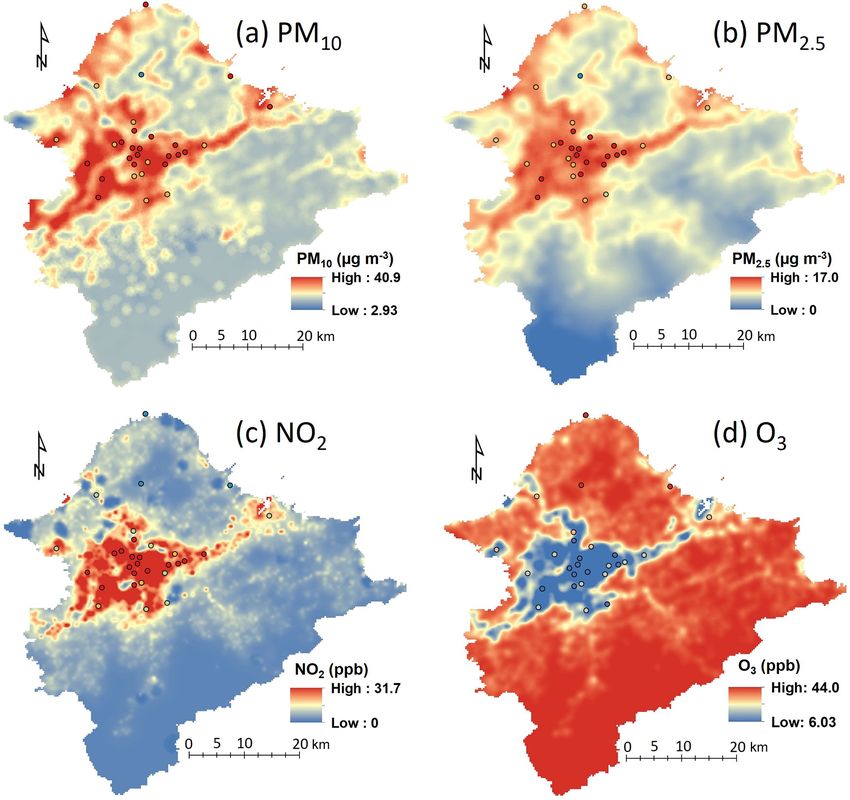
5064                                   Z. Li et al.: Development and intercity transferability of land-use regression models

long-term effect on specific diseases of exposure to air pol-      sible to conduct long-term measurement (e.g., over years) us-
lution require accurate exposure estimates for a large group       ing purpose-designed monitoring networks (Ho et al., 2015;
of participants (e.g., thousands or more) over a defined time      Lee et al., 2017). As a result, a general limitation of LUR
period (Brokamp et al., 2019; Morley and Gulliver, 2018;           models upon purpose-designed monitoring networks is that
Zhou et al., 2020). Different air quality prediction methods,      the established models may only reflect the situation during
such as air dispersion models, atmospheric chemical trans-         the measurement period (Hoek et al., 2008; Shi et al., 2020b).
port models, satellite remote sensing and various statistical      Therefore, the development of long-term average LUR mod-
methods, have been developed and applied to estimate air           els for specific air pollutants using only routine monitoring
pollution (Yim et al., 2019a, b; Tong et al., 2018a, b; Luo        networks should be explored, which is especially critical for
et al., 2018; Shi et al., 2020a) and population exposure (Gu       epidemiological studies.
and Yim 2016; Gu et al., 2018; Hao et al., 2016; Li et al.,           The application of established LUR models to areas out-
2020; Hou et al., 2019; Michanowicz et al., 2016; Wang et          side the study area can reduce extra efforts to develop new
al., 2019, 2020; Yim et al., 2019c). Among these exposure          models (Poplawski et al., 2009). To date, a few studies have
assessment methods, land-use regression (LUR) is a widely          evaluated the transferability of air pollution LUR models
used modeling approach to characterize long-term-average           within a city and between cities or countries (Allen et al.,
air pollutant concentrations at a fine spatial scale, which pro-   2011; Patton et al., 2015; Vienneau et al., 2010; Yang et al.,
vides high-spatial-resolution estimates of exposure for use in     2020). Direct transferability refers to predictor variables and
epidemiological studies (Bertazzon et al., 2015; Eeftens et        coefficients of LUR models both being transferred (Allen et
al., 2016; Jones et al., 2020).                                    al., 2011), whereas transferability with calibration means that
   The LUR method is based on the principle that ambient air       model coefficients are calibrated using air pollutant measure-
pollutant concentrations at fixed-site measurement stations        ments from the target areas (Yang et al., 2020). Direct trans-
are linearly associated with different environmental features      ferability is more meaningful because it can be applied in
(e.g., land use, population density, road network and mete-        areas without air quality measurements (Allen et al., 2011;
orological conditions) surrounding the stations (Anand and         Yang et al., 2020). Previous studies on the transferability of
Monks, 2017; Lu et al., 2020; Naughton et al., 2018; Wu et         LUR models concluded that the predictive performances of
al., 2017). In a city or even at a smaller-spatial-scale area,     LUR models from one area to another were not consistent,
the LUR method is comparable to or sometimes even bet-             ranging from poor (Marcon et al., 2015) to relatively accept-
ter than the approaches of satellite-remote-sensing-based air      able predictive accuracy (Poplawski et al., 2009; Wang et al.,
quality retrievals and air dispersion models in characteriz-       2014). Therefore, more studies should be conducted to assess
ing spatiotemporal variation in air pollution (Marshall et al.,    the transferability of air pollution LUR models.
2008; Shi et al., 2020b). Following feasible procedures of            In this study, annual-average LUR models and spatial-
data processing and analysis, established air pollution LUR        distribution maps were developed for ambient particles of
models can be applied to predict concentrations of air pol-        aerodynamic diameter less than or equal to 10 µm (PM10 ),
lutants at locations without measurements at multiple spatial      PM2.5 , nitrogen dioxide (NO2 ) and ozone (O3 ) in northern
scales or at residential locations of participants in epidemi-     Taiwan in 2019. In addition, the transferability of LUR mod-
ological studies (Li et al., 2021; Liu et al., 2016; Shi et al.,   els between cities in the study area was evaluated. The re-
2020b).                                                            mainder of this paper is organized as follows: the “Materi-
   In recent years, a large number of air pollution LUR stud-      als and methods” section describes the study area, data col-
ies have been conducted in different areas around the world        lection and processing, LUR model establishment and vali-
(Jones et al., 2020; Lee et al., 2017; Liu et al., 2016, 2019;     dation, and prediction of the air pollution exposure surface.
Lu et al., 2020; Miri et al., 2019; Ross et al., 2007; Wu          The “Results and discussion” section presents an overview of
et al., 2017). However, the development and application of         measurement data; established LUR models and their com-
LUR models in the Taiwan region were limited (Hsu et al.,          parison with previous LUR models in Taiwan; the transfer-
2019). In addition, most previous Taiwan LUR studies used          ability of LUR models; the spatial-distribution maps of ambi-
data from purpose-designed monitoring networks or com-             ent PM10 , PM2.5 , NO2 and O3 concentrations; and PM2.5 ex-
bined purpose-designed and routine monitoring networks             posure estimates for a cohort study. The “Conclusions” sec-
(Ho et al., 2015; Lee et al., 2014, 2015). For example, Lee et     tion summarizes the main results and demonstrates the im-
al. (2015) established LUR models for ambient particles of         plications of the present study.
aerodynamic diameter less than or equal to 2.5 µm (PM2.5 )
using a purpose-designed monitoring network of 20 sites
in the Taipei metropolis. The purpose-designed monitoring
campaign has the advantage of capturing short-term air pol-
lution exposure profiles (Jones et al., 2020), but it typically
requires extra human labor and resources (e.g., experimental
materials) (Hoek et al., 2008). Moreover, it is almost impos-

Atmos. Chem. Phys., 21, 5063–5078, 2021                                             https://doi.org/10.5194/acp-21-5063-2021
Z. Li et al.: Development and intercity transferability of land-use regression models                                          5065

2     Materials and methods                                         lected from the Environment Resource database of TWEPA
                                                                    (https://erdb.epa.gov.tw/DataRepository/EnvMonitor/
2.1    Study area                                                   AirQualityMonitorDayData.aspx, last access: 9 July 2020).
                                                                    In addition, hourly concentrations of ambient PM10 ,
The Taipei–Keelung metropolitan area (TKMA), located in             PM2.5 , NO2 and O3 at the local stations from 1 January
northern Taiwan, includes Taipei City, New Taipei City and          to 31 December 2019 were downloaded from the TPEPA
Keelung City. The TKMA is the political, cultural and so-           website      (https://www.tldep.gov.taipei/Public/DownLoad/
cioeconomic center of Taiwan. It covers an area of approx-          AirAutoHour.aspx, last access: 9 July 2020). We calculated
imately 2457 km2 and has 48 administrative districts (Chiu          daily average values of air pollutant concentrations and
et al., 2019; Wang et al., 2018). The TKMA had a popu-              meteorological variables from hourly data and calculated
lation of about 7.03 million in 2019 (TWMOI, 2020), ac-             the annual-average values from daily averaged data for the
counting for approximately 30 % of the total population of          development of LUR models. Daily and annual-average
Taiwan (Fig. 1a). The population densities of Taipei City,          estimates for the air pollutants require at least 75 % data
New Taipei City and Keelung City were 10 175, 2021 and              completeness (Cai et al., 2020); otherwise there was no
2826 people km−2 , respectively, in 2019 (TWMOI, 2020).             value estimate for that day or year.
The numbers of registered motor vehicles were 1.76 mil-                As presented in Table S1 in the Supplement and Fig. 1, the
lion, 3.21 million and 0.28 million in Taipei City, New Taipei      potential predictor variables of the road network, land-use
City and Keelung City, respectively, by the end of 2018             data, normalized difference vegetation index (NDVI), pop-
(TWMOTC, 2020).                                                     ulation density and digital elevation data, which were fre-
   The TKMA is situated in the subtropical region and on            quently used in previous LUR studies, were collected. Land-
the downwind side of mainland China. The built-up area of           use information was taken from the Land Use Investiga-
the TKMA is located in the central part of the Tamsui River         tion of Taiwan conducted by the National Land Surveying
basin, surrounded by mountains, agricultural land and forests       and Mapping Center (https://www2.nlsc.gov.tw/LUI/Home/
(Fig. 1b and c). The characteristics of the basin terrain can       Content_Home.aspx, last access: 9 July 2020). The Taiwan
constrain the diffusion of polluted air masses and thus fa-         land-use status is classified into nine main categories, 41 sub-
vor the accumulation of air pollution in urban areas (Yu and        categories and 103 detailed items. As shown in Fig. 1c, the
Wang, 2010). Local emission sources of air pollutants in the        nine main land-use categories are agriculture, forest, trans-
TKMA include vehicular exhaust, industrial emissions and            portation, water bodies, built-up areas, public utilities, recre-
various sources related to residential activities (e.g., cook-      ation, mining or salt production, and others (Chen et al.,
ing) (Chen et al., 2020; Ho et al., 2018; Wu et al., 2017). In      2020). The road network from the Taiwan Ministry of Trans-
winter time, the long-distance transport of dust and polluted       portation and Communications includes three types of road:
air masses under the northeast monsoon from the Asian con-          local roads, major roads and expressways (Fig. 1d). The
tinent results in a significant increase in concentrations of air   NDVI and elevation data were extracted from the database
pollutants (Chi et al., 2017; Chou et al., 2010).                   of the Resources and Environmental Sciences Data Center,
                                                                    Chinese Academy of Sciences (http://www.resdc.cn, last ac-
2.2    Data collection and processing                               cess: 9 July 2020).
                                                                       The values of potential predictor variables in buffer sizes
The Taiwan Environmental Protection Administration                  of 50, 100, 300, 500, 700, 1000, 2000, 3000, 4000 and
(TWEPA) operates 20 central air-quality-monitoring stations         5000 m surrounding the sampling stations were summarized
in the TKMA, of which 12 stations are in New Taipei                 for use in LUR model development. To ensure the consis-
City, 7 are in Taipei City, and 1 station is in Keelung             tency of results between model training and cross-validation,
City (https://airtw.epa.gov.tw/ENG/default.aspx, last ac-           we included only the potential predictor variables with at
cess: 9 July 2020). In addition, the Taipei Environmental           least seven stations (i.e., around 25 % of all stations) exhibit-
Protection Agency (TPEPA) operates 10 local air-quality-            ing different values and where the minimum or maximum
monitoring stations (https://www.tldep.gov.taipei/EIACEP_           values lay within three times the 10th to the 90th percentile
EN/Air_NormalStation.aspx, last access: 9 July 2020).               range below or above the 10th and the 90th percentile (Wolf
In total, these stations include 21 general stations, 6 traf-       et al., 2017).
fic stations, 2 background stations and 1 country park
station (Fig. 1a). Detailed descriptions of sampling sta-           2.3   Model development and validation
tions, measurement instruments, and quality assurance
and control procedures are available in TWEPA (2020).               The LUR models of ambient PM10 , PM2.5 , NO2 and O3
Hourly measurements of ambient PM10 , PM2.5 , NO2 and               for the entire study area (the area-specific LUR models)
O3 concentrations and the meteorological variables of               were established using all 30 air-quality-monitoring stations.
temperature, wind speed and relative humidity at the central        In addition, city-specific LUR models for New Taipei City
stations from 1 January to 31 December 2019 were col-               and Keelung City were developed using the 13 air-quality-

https://doi.org/10.5194/acp-21-5063-2021                                             Atmos. Chem. Phys., 21, 5063–5078, 2021
5066                                    Z. Li et al.: Development and intercity transferability of land-use regression models

Figure 1. The characteristics of the study area. (a) Population density and the location of air-quality-monitoring stations. A total of 30
air-quality-monitoring stations were included in this study. (b) Digital elevation. (c) Land-use types. (d) The road network.

monitoring stations located in these two cities, and the estab-        included, and meanwhile the predictive accuracy of the es-
lished models were directly transferred to Taipei City. Sim-           tablished model is maximized. In brief, all potential predic-
ilarly, city-specific LUR models for Taipei City were devel-           tor variables were included as candidate independent vari-
oped using the 17 quality-monitoring stations located in this          ables, and a prior direction was assigned for each category
city, and the established models were directly transferred to          of variable based on the atmospheric mechanism. The model
New Taipei City and Keelung City. In this study, we did                construction started by including the predictor variable with
not consider the calibration of model coefficients because we          the highest adjusted explained variance (R 2 ). The remaining
planned to evaluate the direct transferability of city-specific        predictor variables were entered into the model if they met
LUR models to another nearby city area when there were no              all of the following criteria: (1) the gain of the adjusted R 2
routine air quality measurements.                                      was no less than 1 %; (2) the direction of effect of the predic-
   There is no standard modeling method for developing                 tor variable was pre-defined; (3) variables were added into
LUR models (Hoek et al., 2008). In this study, the supervised          the model when the probability of F was less than 0.05 and
forward linear regression method (Cai et al., 2020; Eeftens            removed when the probability of F was greater than 0.10;
et al., 2016; Xu et al., 2019) was used to develop the LUR             (4) variables already included in the model retained the same
models. This modeling method can ensure that only predic-              direction of effect; and (5) following previous studies (Chen
tor variables following the plausible direction of effect are          et al., 2020; Marcon et al., 2015; Wang et al., 2014), the

Atmos. Chem. Phys., 21, 5063–5078, 2021                                                   https://doi.org/10.5194/acp-21-5063-2021
Z. Li et al.: Development and intercity transferability of land-use regression models                                                                     5067

predictor variables with variance inflation factor (VIF) val-      Table 1. Statistical description of measured air pollutants by differ-
ues larger than 3 were dropped to make a tradeoff between          ent types of stations.
model interpretation and the predictive accuracy (Eeftens et
al., 2016). Multiple buffer sizes of a specific variable (e.g.,      Air pollutant           Station type           N      Mean         SD      Min      Max
the length of local roads) could be selected in the final model      PM10    (µg m−3 )       General                21       28.5     2.84      22.3      35.0
as long as they followed the selection criteria (Henderson et                                Traffic                 6       33.6     4.57      27.3      40.3
al., 2007).                                                                                  Background              2       39.3     2.11      37.8      40.8
                                                                                             Country park∗           1       15.7        –         –         –
   Standard diagnostic tests were applied to ensure that the
LUR models were reasonably established (Li, 2020; Wolf               PM2.5 (µg m−3 )         General                21       13.7     1.36      10.6      15.4
                                                                                             Traffic                 6       16.8     2.98      13.3      21.3
et al., 2017). The Cook’s distance value was calculated to
                                                                                             Background              2       13.2     0.44      12.9      13.6
detect the outliers of data points (i.e., stations) (Jones et                                Country park            1       8.06        –         –         –
al., 2020). Air pollutant observations with a Cook’s distance
                                                                     NO2 (ppb)               General                21       14.3     3.32      7.86      21.7
value greater than 1 would be excluded, and the LUR model                                    Traffic                 6       24.6     6.16      17.1      32.2
for this air pollutant would be re-established (Weissert et al.,                             Background              2       3.81     1.28      2.90      4.71
2018; Wolf et al., 2017). In addition, Moran’s I values on                                   Country park            1       1.89        –         –         –
the concentration residuals of the final LUR models were             O3 (ppb)                General                21       29.4     3.51      23.6      35.5
calculated using ArcGIS software to evaluate the spatial au-                                 Traffic                 4       21.6     5.48      15.2      28.0
tocorrelation (Bertazzon et al., 2015; Lee et al., 2017; Liu                                 Background              2       41.7     0.70      41.2      42.2
                                                                                             Country park            1       39.8        –         –         –
et al., 2016). The R 2 and root mean square error (RMSE)
                                                                   N means the number of stations for this type; SD means the standard deviation; min and max
were estimated to evaluate the performance of the models           refer to the minimum and maximum values of the air pollutant concentrations, respectively.
                                                                   ∗ There is only one country park station; therefore there are no estimates of SD, min and max
(Li et al., 2021). Furthermore, leave-one-out cross-validation     values.
(LOOCV) was employed to evaluate the predictive capacity
of the LUR models (Liu et al., 2019; Shi et al., 2020b; Yang
et al., 2020).                                                     has relatively good representativeness. The annual-average
   Spatial analysis and calculations were performed using          PM10 concentration of 39.3 µg m−3 at background stations
ArcGIS software, version 10.6 (ESRI Inc., Redlands, CA,            was the highest, followed in descending order by traffic sta-
USA). The statistical analysis was performed using R soft-         tions with 33.6 µg m−3 , general stations with 28.5 µg m−3
ware, version 3.5.2 (R Core Team, 2018).                           and the country park station with 15.7 µg m−3 . The traffic
                                                                   stations and country park station had the highest and low-
2.4    Air pollution surface prediction                            est annual-average PM2.5 concentrations, respectively. The
                                                                   annual-average PM2.5 concentrations at general stations of
The entire study area of the TKMA was divided into 9839            13.7 µg m−3 and background stations of 13.2 µg m−3 were
500 m × 500 m grid cells. The air pollutant concentrations at      comparable. Except for the country park station, the annual-
the centroids of the grid cells were estimated using the estab-    average PM10 and PM2.5 concentrations at other types of
lished area-specific LUR models. When the LUR models es-           stations were higher than the air quality guidelines (AQGs)
timated negative concentration values, the concentration val-      for PM10 and PM2.5 of 20.0 and 10.0 µg m−3 , respectively,
ues of the grid cells were set to 0; when air pollutant con-       proposed by the World Health Organization (WHO) (WHO,
centration estimates exceeded the maximum observed con-            2006). The annual-average NO2 concentration of 24.6 ppb at
centrations by more than 20 %, the concentrations of grid          the traffic stations was the highest, followed by general sta-
cells were set to 120 % of the maximum observed concen-            tions with 14.3 ppb. The annual-average NO2 concentrations
trations (Henderson et al., 2007). The area-specific LUR-          at background stations (3.81 ppb) and the country park sta-
model-based negative and high concentration estimates ac-          tion (1.89 ppb) were significantly lower than those of gen-
counted for only 0 %, 4 %, 2 % and 0 % of PM10 , PM2.5 , NO2       eral and traffic stations because they were farther away from
and O3 estimates, respectively. Then the spatial-distribution      traffic emissions. The annual-average NO2 concentration at
maps of ambient PM10 , PM2.5 , NO2 and O3 concentrations           traffic stations (24.6 ppb) was slightly higher than the WHO
were created using the kriging interpolation method (Cai et        NO2 AQG of 40.0 µg m−3 (about 21.3 ppb) (WHO, 2006),
al., 2020).                                                        while other types of stations had annual-average NO2 con-
                                                                   centrations lower than this AQG. In contrast to NO2 , the
3     Results and discussion                                       background stations (41.7 ppb) and the country park sta-
                                                                   tion (39.8 ppb) had higher annual-average O3 concentrations
3.1    Descriptive statistics of the air quality data              than those of traffic stations (21.6 ppb) or general stations
                                                                   (29.4 ppb) (Table 1).
In general, the included air-quality-monitoring stations were
situated at different types of land use across the TKMA (Ta-
ble 1 and Fig. 1c), which suggests that the collected data set

https://doi.org/10.5194/acp-21-5063-2021                                                    Atmos. Chem. Phys., 21, 5063–5078, 2021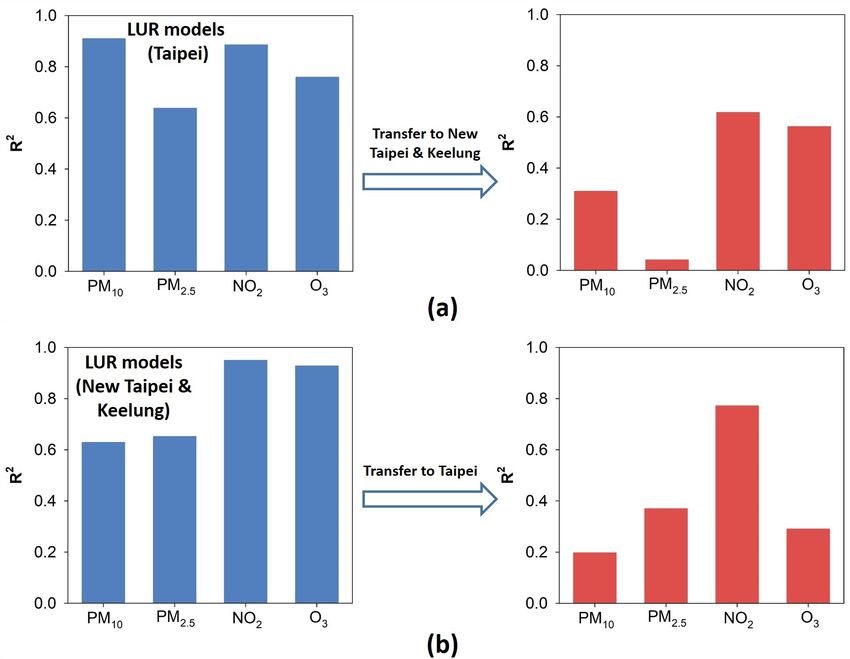
5068 Z. Li et al.: Development and intercity transferability of land-use regression models
3.2 The area-specific LUR models size of 2000 m, the area of transportation land in a buffer size
of 100 m and the area of water body land in a buffer size
Figure S1 in the Supplement shows that Cook’s distance val- of 500 m. The PM2.5 LUR model included the area of trans-
ues were below 1 for all the stations of the area-specific portation land within a 300 m buffer, the area of major roads
LUR models, suggesting that there were no station outliers within a 100 m buffer, the area of forest land within a 700 m
in developing these LUR models. For PM10 and PM2.5 LUR buffer, the area of recreational land within a 2000 m buffer
models, Cook’s distance values ranged from almost 0.00 to and the distance to the nearest major roads. For PM10 and
around 0.72. The Cook’s distance values of the NO2 LUR PM2.5 LUR models, the direction of effect for transportation
model were between almost 0.00 and 0.28, whereas the land and traffic roads was positive, while the direction of ef-
Cook’s distance values of the O3 LUR model were between fect of other predictor variables was negative. Forest and ur-
almost 0.00 and 0.38 (Fig. S1). The final area-specific LUR ban green space land (i.e., recreational land) were included in
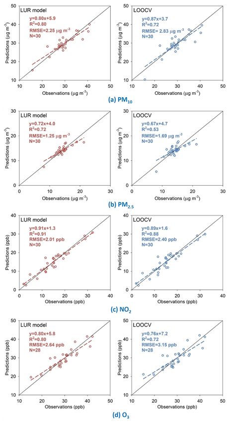
models and their corresponding predictive accuracy are sum- both PM10 and PM2.5 LUR models (Table 2). Ji et al. (2019),
marized in Table 2 and Fig. 2. The model R 2 values ranged Jones et al. (2020) and Miri et al. (2020) included forest land
from 0.72 for PM2.5 to 0.91 for NO2 , indicating a good fit or urban green space as the predictor variables in their final
for all air pollutants. PM10 , NO2 and O3 LUR models per- city-scale PM LUR models, demonstrating the mitigation ef-
formed well, with LOOCV R 2 values being < 0.10 lower fect of these land-use types on PM concentrations. Chen et
than the model R 2 values. For PM2.5 , the model was not al. (2019) and Jeanjean et al. (2016) reported the effective-
as robust as those of other air pollutants, with the LOOCV ness of urban green space in mitigating PM pollution. The
R 2 value being 0.19 lower than the model R 2 value (Fig. 2). water body type of land use reduced PM10 concentrations,
The reason for this is that the PM2.5 concentrations among as evidenced by the negative regression coefficient (Table 2).
the stations were not as discrete as those of other air pollu- The water bodies can make PM10 absorb moisture and in-
tants (Table 1 and Fig. 2). The significance of the predictor crease sedimentation. In addition, large areas of water pro-
variables (p value) and VIF values all met the requirements vide good conditions for the dispersion of air pollutants (Zhu
for LUR model development. Moran’s I values were 0.0047, and Zhou, 2019).
−0.072, 0.023 and −0.055 for the LUR models of ambient For the NO2 LUR model, the four predictor variables in-
PM10 , PM2.5 , NO2 and O3 . In addition, z-score values were cluded were the area of transportation land in buffer sizes
0.83, −0.79, 1.2 and −0.34 for ambient PM10 , PM2.5 , NO2 of 3000 and 50 m, the area of recreational land in a 1000 m
and O3 LUR models, respectively, indicating that the spatial buffer, and the sum of the length of local roads in a 1000 m
patterns of concentration residuals of the LUR models do not buffer. The direction of effect for the recreational land was
appear to be significantly different from random (Fig. S2). negative, while other predictor variables showed a positive
The final area-specific LUR models consisted of three (for effect (Table 2). The O3 LUR model included predictor vari-
O3 ), four (for NO2 ) and five predictor variables (for PM10 ables with relatively small buffer sizes of less than 700 m.
and PM2.5 ) (Table 2). Consistent with the previous LUR The three predictor variables were the area of transportation
studies of De Hoogh et al. (2018), Eeftens et al. (2016), Jones land in buffer sizes of 700 and 50 m and the area of public
et al. (2020), Weissert et al. (2018) and Wolf et al. (2017), utilization land within a 300 m buffer. The directions of ef-
the established LUR models contained at least one traffic- fect for these three variables were all negative (Table 2). The
related predictor variable in buffer sizes ranging from 50 to traffic-related predictor variables were important variables in
3000 m. Traffic emission is a major source of air pollution predicting NO2 and O3 concentrations but in different direc-
in urban areas of the TKMA (Lee et al., 2014; Wu et al., tions of effect. Consistent with previous studies by De Hoogh
2017). For instance, it was reported that gasoline and diesel et al. (2016), Eeftens et al. (2016), Lee et al. (2014) and Liu
vehicle emissions contributed approximately half of PM2.5 et al. (2019), the established NO2 LUR model also revealed
concentrations in Taipei City based on source apportionment the mitigation effect of urban green space (i.e., recreational
analysis (Ho et al., 2018). Several previous LUR studies se- land) on NO2 concentration.
lected the population density variable as the final explanatory A comparison of this study with previous LUR studies
variable in their PM2.5 and NO2 LUR models (Ji et al., 2019; in Taiwan is presented in Table S2. The predictive perfor-
Meng et al., 2015; Rahman et al., 2017). However, it was not mance of the LUR model for ambient PM10 in this study was
included in our final LUR models. A possible explanation is slightly worse than that of Lee et al. (2015), with an R 2 value
that the population density variable is moderately or highly of 0.87. In addition, the R 2 and LOOCV R 2 values (0.72
correlated with the variables (e.g., the area of recreational and 0.53, respectively) of the PM2.5 LUR model in this study
land) included in our final LUR models. were lower than those of Ho et al. (2015) (an R 2 value of
As shown in Table 2, PM10 and PM2.5 LUR models in- 0.75 and an LOOCV R 2 value of 0.62), Lee et al. (2015) (an
cluded predictor variables of both small and large buffer R 2 value of 0.95 and an LOOCV R 2 value of 0.91) and Wu
sizes. The LUR model for PM10 included the area of for- et al. (2017) (an R 2 value of 0.90 and an LOOCV R 2 value
est land in a buffer size of 300 m, the area of built-up land in of 0.83) but higher than that of Wu et al. (2018), with an R 2
a buffer size of 50 m, the area of recreational land in a buffer value of 0.66. The NO2 LUR model performed better than
Atmos. Chem. Phys., 21, 5063–5078, 2021 https://doi.org/10.5194/acp-21-5063-2021Z. Li et al.: Development and intercity transferability of land-use regression models 5069
Table 2. Description of the 2019 annual-average LUR models for ambient PM10 , PM2.5 , NO2 and O3 in the TKMA.
Air pollutant Variables Coefficient Standard error p VIF Predictive accuracy
PM10 (constant) 38.5 1.4 < 0.001 NA
LU2_300 −7.71E-05 1.20E-05 < 0.001 1.4 R 2 = 0.80;
LU5_50 1.01E-03 4.39E-04 0.031 1.3 RMSE = 2.25;
LU7_2000 −7.06E-06 1.29E-06 < 0.001 1.8 LOOCV R 2 = 0.72;
LU3_100 5.33E-04 1.19E-04 < 0.001 1.7 LOOCV RMSE = 2.83.
LU4_500 −2.97E-05 9.82E-06 0.006 1.1
PM2.5 (constant) 13.7 1.0 < 0.001 NA
LU3_300 4.26E-05 1.25E-05 0.002 1.7 R 2 = 0.72;
R2_100 3.52E-04 1.05E-04 0.003 1.2 RMSE = 1.25;
LU2_700 −4.65E-06 1.34E-06 0.002 1.6 LOOCV R 2 = 0.53;
LU7_2000 −2.20E-06 8.03E-07 0.012 2.2 LOOCV RMSE = 1.69.
Dis_Major −5.70E+01 2.69E+01 0.045 1.1
NO2 (constant) 0.70 1.21 0.570 NA
R 2 = 0.91;
LU3_3000 1.77E-06 2.80E-07 < 0.001 2.4
RMSE = 2.01;
LU3_50 2.35E-03 2.68E-04 < 0.001 1.3
LOOCV R 2 = 0.88;
LU7_1000 −1.88E-05 3.30E-06 < 0.001 1.5
LOOCV RMSE = 2.40.
RL3_1000 4.91E-05 1.55E-05 0.004 2.0
O3 (constant) 44.0 1.7 < 0.001 NA R 2 = 0.80;
LU3_700 −2.88E-05 4.00E-06 < 0.001 1.1 RMSE = 2.64;
LU3_50 −2.00E-03 3.65E-04 < 0.001 1.1 LOOCV R 2 = 0.72;
LU6_300 −3.07E-05 1.20E-05 0.018 1.0 LOOCV RMSE = 3.15.
LU2_300, LU2_700: the area of forest in buffer sizes of 300 m and 700 m. LU5_50: the area of built-up land in a buffer size of 50 m. LU7_1000 and
LU7_2000: the area of recreational land in buffer sizes of 1000 and 2000 m. LU3_50, LU3_100, LU3_300, LU3_700 and LU3_3000: the area of
transportation land in buffer sizes of 50, 100, 300, 700 and 3000 m. LU4_500: the area of water body in a buffer size of 500 m. R2_100: the area of
major roads in a buffer size of 100 m. Dis_Major: the distance to the nearest major roads. RL3_1000: the length of local roads in a buffer size of
1000 m. LU6_300: the area of public utilization land in a buffer size of 300 m. VIF: the variance inflation factor. LOOCV: leave-one-out
cross-validation. RMSE: root mean square error. NA: not available.
that of Lee et al. (2014) and was comparable to that of Chen for each specific air pollutant, the predictive performance
et al. (2020). Hsu et al. (2019) developed an O3 LUR model of these city-specific LUR models can be slightly higher or
for the whole Taiwan region, with an R 2 value of 0.74 (Hsu lower than those of the area-specific LUR models. Figure 3
et al., 2019). Our study established a reasonable LUR model shows the transferability of LUR models between Taipei City
for ambient O3 in the TKMA with an R 2 value of 0.80 and an and New Taipei City and Keelung City. The city-specific
LOOCV R 2 value of 0.70, which is a relatively high predic- LUR models performed worse in another city area than in
tive performance. Compared with PM10 , PM2.5 and NO2 , the the city where these models were established. For instance,
establishment of O3 LUR models has been limited in these the transfer-predictive R 2 values of the Taipei LUR models
previous Taiwan LUR studies (Table S2) or in most of the were 0.31, 0.04, 0.62 and 0.56 for predicting ambient PM10 ,
LUR studies in other areas, but it is essential to establish O3 PM2.5 , NO2 and O3 in New Taipei City and Keelung City,
LUR models given that O3 is a toxic photochemical pollu- respectively (Fig. 3). These values were substantially lower
tant threatening human health and the ecosystem (Ning et than the corresponding R 2 values of the Taipei LUR models.
al., 2020; Yim et al., 2019b). The NO2 LUR models showed good transferability between
the two city areas, with transfer-predictive R 2 values higher
3.3 Transferability of the city-specific LUR models than 0.62. However, the PM10 , PM2.5 and O3 LUR models
performed poorly when they were transferred between the
The city-specific LUR models for ambient PM10 , PM2.5 , two city areas, with transfer-predictive R 2 values of < 0.31,
NO2 and O3 in Taipei City, New Taipei City and Keelung < 0.37 and < 0.56, respectively (Fig. 3). Similar to the pre-
City are shown in Tables S3 and S4, respectively. The model vious studies of Marcon et al. (2015) and Yang et al. (2020),
R 2 values of the Taipei City PM10 , PM2.5 , NO2 and O3 these results suggested that there may be large uncertainties
LUR models were 0.91, 0.64, 0.89 and 0.76, respectively in transferring LUR models between cities and even between
(Table S3), while the New Taipei City and Keelung City nearby cities with similar geographic and urban-design char-
PM10 , PM2.5 , NO2 and O3 LUR models had R 2 values of acteristics. The use of novel cost-effective methods (e.g.,
0.63, 0.65, 0.95 and 0.93, respectively (Table S4). In general, low-cost air quality sensors or a satellite remote-sensing ap-
https://doi.org/10.5194/acp-21-5063-2021 Atmos. Chem. Phys., 21, 5063–5078, 20215070 Z. Li et al.: Development and intercity transferability of land-use regression models Figure 2. A comparison of LUR-predicted concentrations and observed concentrations of the studied air pollutants and the LOOCV-predicted concentrations and observed concentrations of the studied air pollutants. (a) PM10 , (b) PM2.5 , (c) NO2 and (d) O3 . N is the sample size, and the solid line is the 1 : 1 line. Atmos. Chem. Phys., 21, 5063–5078, 2021 https://doi.org/10.5194/acp-21-5063-2021
Z. Li et al.: Development and intercity transferability of land-use regression models 5071
Figure 3. The changes in R 2 values for direct transfer of ambient PM10 , PM2.5 , NO2 and O3 LUR models between Taipei City and New
Taipei City and Keelung City.
proach) is therefore recommended to assess air pollution and Table 3. Pearson correlation coefficients (PCCs) among the esti-
associated population exposure in cities with limited fixed- mated concentrations of ambient PM10 , PM2.5 , NO2 and O3 .
site measurement stations.
Air pollutant PM10 PM2.5 NO2 O3
3.4 Spatial maps
PM10 1 0.775∗∗ 0.719∗∗ −0.730∗∗
PM2.5 1 0.761∗∗ −0.775∗∗
LUR-model-derived air-pollution-spatial-distribution maps
NO2 1 −0.920∗∗
provide valuable and useful air pollutant concentration sur- O3 1
faces in the TKMA. In general, there was a good agreement
between LUR-model-based concentration estimates and ob- ∗∗ Correlation is significant at the 0.01 level (two-tailed).
servations for PM10 , PM2.5 , NO2 and O3 (Fig. 4). For PM10
and PM2.5 , there were certain differences between LUR-
model-based concentration estimates and observations at the which documented that high PM2.5 concentrations were dis-
country park station (Fig. 4). A possible reason for this differ- tributed mainly in the urban areas of the TKMA, and there
ence may be that the kriging interpolation method removed were also scattered points of high PM2.5 concentrations in
low-concentration estimates at this small area when the con- its outer ring. However, the estimated 2019 annual-average
centration estimates at nearby areas were higher. PM2.5 concentrations in this study were significantly lower
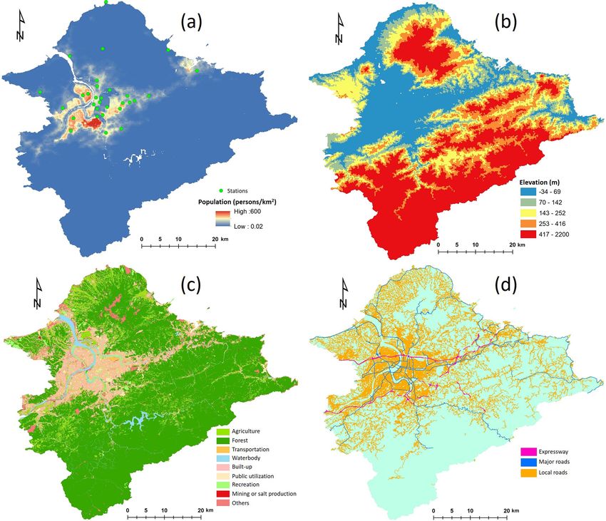
High concentrations of ambient PM10 , PM2.5 and NO2 than those for 2006–2012 estimated by Wu et al. (2017).
were predicted in the urban areas of Taipei City, New Taipei There was a clear decreasing trend in PM2.5 concentrations
City and Keelung City and along the road network. The es- in the whole of Taiwan over the past decade (Ho et al., 2020;
timated PM10 and PM2.5 concentrations in urban areas were Jung et al., 2018). For example, Jung et al. (2018) reported
around 35.0 to 40.9 µg m−3 and around 12.0 to 17.0 µg m−3 , that the estimated PM2.5 concentrations declined by 1.7 and
respectively, whereas the urban areas had NO2 concentra- 1.6 µg m−3 in the morning and afternoon, respectively, per
tions of around 12.0 to 31.7 ppb (Fig. 4). This spatial- year over the whole of Taiwan during the period 2005–2015.
distribution pattern is understandable given that the traffic- O3 showed a generally opposite spatial-variability pattern
related predictor variables were included in the final PM10 , compared with the other three air pollutants, with lower con-
PM2.5 and NO2 LUR models. A similar spatial pattern of centrations (< about 32.0 ppb) in urban areas than in rural
PM2.5 concentrations was reported by Wu et al. (2017), areas (Fig. 4). A possible explanation for this finding is that
https://doi.org/10.5194/acp-21-5063-2021 Atmos. Chem. Phys., 21, 5063–5078, 20215072 Z. Li et al.: Development and intercity transferability of land-use regression models
Figure 4. The spatial distribution of ambient air pollutant concentrations derived from established LUR models. (a) PM10 , (b) PM2.5 ,
(c) NO2 and (d) O3 . The colored circles represent the observations from stations.
high concentrations of NO and NO2 in urban areas react with 3.5 Air pollutant exposure estimates for a cohort study
O3 , resulting in a decrease in O3 concentration (Hsu et al.,
2019; Vardoulakis et al., 2011).
Air pollutant concentrations measured at nearby fixed-site
Correlations of estimated concentrations of PM10 , PM2.5 ,
stations are often used to represent exposures in epidemi-
NO2 and O3 in the TKMA are shown in Table 3. Consistent
ological studies (Lin et al., 2016; Shi et al., 2020c), but
with previous studies by Hoek et al. (2008), Lu et al. (2020),
the spatial resolution of these estimates is relatively coarse
Vardoulakis et al. (2011) and Wolf et al. (2017), the spatial-
due to the limited number of sampling stations (Bertazzon
distribution maps revealed high spatial correlations among
et al., 2015). In recent years, LUR modeling has become
the four air pollutants. PM10 concentrations had strong pos-
a more widely applied method to estimate air pollution ex-
itive correlations with PM2.5 and NO2 , suggesting common
posures at a fine spatial scale (Lee et al., 2014; Wolf et
sources of these three air pollutants. In contrast to this, PM10
al., 2017). Figure S3 shows that there are differences be-
concentrations were negatively correlated with O3 concentra-
tween LUR-model-based air pollution exposure estimates
tions, with a Pearson correlation coefficient (PCC) value of
and nearby-station measurements at residential locations of
−0.730. Similarly, PM2.5 concentrations had a strong posi-
participants in a cohort study conducted in the TKMA. The
tive correlation with NO2 concentrations but showed a sig-
average values of the LUR-estimated PM10 , PM2.5 , NO2 and
nificant negative correlation with O3 concentrations. The
O3 exposure concentrations were 36.0 µg m−3 , 14.2 µg m−3 ,
concentrations of NO2 and O3 were negatively correlated
18.0 ppb and 29.2 ppb, respectively, whereas the corre-
because of the NOx titration effect in urban areas, with a
sponding nearby-station measurements were 27.7 µg m−3 ,
PCC value of −0.920. Similar findings were reported by
13.8 µg m−3 , 16.3 ppb and 28.6 ppb, respectively (Table S5).
De Hoogh et al. (2018) and Lu et al. (2020).
Compared with LUR-model-based estimates, the nearby-
station measurements underestimated PM10 , PM2.5 , NO2
and O3 exposures of cohort participants by 8.23 µg m−3 ,
0.41 µg m−3 , 1.73 ppb and 0.60 ppb, respectively (Table S5).
Atmos. Chem. Phys., 21, 5063–5078, 2021 https://doi.org/10.5194/acp-21-5063-2021Z. Li et al.: Development and intercity transferability of land-use regression models 5073
3.6 Limitations
This study is subject to several limitations. First, apart from
the variables used in this study, more predictor variables
(e.g., localized emission data and urban building morphology
data) should be included and tested to develop LUR models.
For example, Wu et al. (2017) and Chen et al. (2020) assessed
the roles of two culturally specific emission sources, Chi-
nese restaurants and temples, on the development of ambient
PM2.5 and NO2 LUR models in Taiwan. More studies should
be conducted to test the influence of different potential pre-
dictor variables on the development of LUR models (Hoek
et al., 2008). Second, like most linear regression techniques,
the supervised forward linear regression method is not pro-
ficient in modeling extreme values (Jones et al., 2020). In
addition, there may be complex and non-linear relationships
between the explanatory variables and air pollutant concen-
trations (Wang et al., 2020). Other types of linear regres-
sion methods (Hoek et al., 2008; Shi et al., 2020b) and the
novel machine learning algorithms (Wang et al., 2020) can be
tested in estimating surface-level air pollutant concentrations
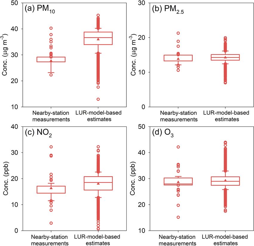
Figure 5. Box plots of nearby-station air pollutant measurements
in the further study. Third, the kriging interpolation method
and LUR-model-based estimates of air pollutant concentration.
(a) PM10 , (b) PM2.5 , (c) NO2 and (d) O3 . The triangle symbol in tends to remove air pollutant peak concentrations, resulting
each box is the mean value, the solid line is the median value, the in an underestimation of air pollution exposure at pollution
box extends from the 25th to the 75th percentile, the whiskers (er- hot spots. Other spatial-mapping methods should be consid-
ror bars) below and above the box are the 10th and 90th percentiles, ered in further studies. It is recommended that air pollutant
and the lower and upper cycle symbols are outliers. concentrations at residential locations of participants should
be estimated directly for cohort studies. Fourth, there may
be uncertainty in spatial estimations of air pollutant concen-
In addition, the concentration ranges of LUR-estimated trations with a limited number of sampling stations. Further
annual-average PM10 (13.0–45.2 µg m−3 ), PM2.5 (6.96– studies are warranted to evaluate the influence of the number
19.9 µg m−3 ), NO2 (0.70–32.2 ppb) and O3 (17.5–44.0 ppb) of sampling stations and their spatial distributions on the de-
exposure concentrations were larger than those of nearby- velopment of LUR models and the air pollution spatial maps.
station measurements for PM10 (22.3–40.3 µg m−3 ), PM2.5
(10.6–21.3 µg m−3 ), NO2 (2.90–32.2 ppb) and O3 (15.2–
42.2 ppb) (Table S5 and Fig. 5). This indicates that the LUR- 4 Conclusions
model-based exposure estimates can capture the large spatial
variability in air pollutant exposure among the cohort par- Following standard development procedures, the annual-
ticipants. Similar findings have been reported in studies of average LUR models of ambient PM10 , PM2.5 , NO2 and
Lee et al. (2014) and Marshall et al. (2008). Furthermore, the O3 were established in the TKMA of northern Taiwan using
LUR-model-based PM10 , PM2.5 , NO2 and O3 exposure esti- only data from the routine monitoring network. These LUR
mates and nearby-station measurements were weakly corre- models were reasonable, based on the evaluation metrics of
lated, with linear regression R 2 values ranging from 0.05 for Cook’s distance, VIF, Moran’s I and p values. The R 2 val-
PM10 to 0.19 for NO2 (Fig. 6). A possible explanation is that ues of the LUR models for ambient PM10 , PM2.5 , NO2 and
LUR-model-based exposure estimates generally accounted O3 were 0.80, 0.72, 0.91 and 0.80, respectively. The traffic-
for neighborhood-scale variations in air pollutant concentra- related predictor variables were the major explanatory factors
tions, while the nearby-station measurements usually only in the LUR models for all the studied air pollutants.
revealed the urban-scale variability in air pollution (e.g., ur- The predictive performance varied greatly among air pol-
ban area versus suburban area versus rural area) (Marshall lutants in examining the transferability of city-specific LUR
et al., 2008). The LUR-model-based exposure estimates and models between New Taipei City and Keelung City and
nearby-station measurements should be further validated if Taipei City, with relatively high transfer-predictive R 2 values
the air quality measurement data at residential locations of for NO2 . Therefore, this study highlights that the established
cohort participants (if not all, at least some of the partici- LUR models in a city area can result in a large estimation
pants) are available. bias when applied to another nearby city area with similar
geographic and urbanization conditions. The transferability
https://doi.org/10.5194/acp-21-5063-2021 Atmos. Chem. Phys., 21, 5063–5078, 20215074 Z. Li et al.: Development and intercity transferability of land-use regression models
Figure 6. The linear regression of nearby-station air pollutant measurements and LUR-model-based air pollutant concentration estimates.
(a) PM10 , (b) PM2.5 , (c) NO2 and (d) O3 .
may even be uncertain in a city with complex terrain (Yim Supplement. The supplement related to this article is available on-
et al., 2007, 2014). It is necessary to conduct more studies line at: https://doi.org/10.5194/acp-21-5063-2021-supplement.
to evaluate and improve the intercity transferability of LUR
models.
The spatial-distribution maps of the four air pollutants Author contributions. SHLY planned, supervised and sought fund-
showed that the developed LUR models are reasonable in ing for this study. ZL performed the data analysis and prepared the
modeling the spatial variabilities in air pollution. Ambient paper with contributions from all co-authors.
PM10 , PM2.5 and NO2 shared similar spatial variations, with
relatively high concentrations in urban areas and along the
Competing interests. The authors declare that they have no conflict
road network. Ambient O3 presented a generally opposite
of interest.
spatial variability compared with PM10 , PM2.5 and NO2 .
These estimated air pollution concentration surfaces provide
information for the management of air pollution and expo- Special issue statement. This article is part of the special issue “Air
sure estimates for epidemiological studies. Compared with Quality Research at Street-Level (ACP/GMD inter-journal SI)”. It
nearby-station measurements, the LUR-model-based con- is not associated with a conference.
centration estimates captured a wider range of exposure to
PM10 , PM2.5 , NO2 and O3 for participants in a cohort study
in the TKMA. Further studies should pay more attention Acknowledgements. We would like to thank the Taiwan Environ-
to utilizing other data sources (e.g., satellite remote-sensing mental Protection Administration for providing air quality and me-
data) with comprehensive spatiotemporal coverage to vali- teorological data.
date the LUR-model-based estimations of air pollutant con-
centrations.
Financial support. This work is funded by the Vice-Chancellor’s
Discretionary Fund of The Chinese University of Hong Kong (grant
Data availability. The model data presented in this article are avail- no. 4930744), the Dr. Stanley Ho Medicine Development Founda-
able from the authors upon request (yimsteve@gmail.com). tion (grant no. 8305509), and the project from the ENvironmental
SUstainability and REsilience (ENSURE) partnership between the
CUHK and UoE.
Atmos. Chem. Phys., 21, 5063–5078, 2021 https://doi.org/10.5194/acp-21-5063-2021Z. Li et al.: Development and intercity transferability of land-use regression models 5075
Review statement. This paper was edited by Sunling Gong and re- and BC models for Western Europe–Evaluation of spatiotempo-
viewed by two anonymous referees. ral stability, Environ. Int., 120, 81–92, 2018.
Eeftens, M., Meier, R., Schindler, C., Aguilera, I., Phuleria, H.,
Ineichen, A., Davey, M., Ducret-Stich, R., Keidel, D., Probst-
Hensch, N., and Künzli, N.: Development of land use regression
models for nitrogen dioxide, ultrafine particles, lung deposited
References surface area, and four other markers of particulate matter pollu-
tion in the Swiss SAPALDIA regions, Environ. Health, 15, 53,
Allen, R. W., Amram, O., Wheeler, A. J., and Brauer, M.: The trans- https://doi.org/10.1186/s12940-016-0137-9, 2016.
ferability of NO and NO2 land use regression models between Gu, Y. and Yim, S. H. L.: The air quality and health impacts of
cities and pollutants, Atmos. Environ., 45, 369–378, 2011. domestic trans-boundary pollution in various regions of China,
Anand, J. S. and Monks, P. S.: Estimating daily surface NO2 con- Environ. Int., 97, 117–124, 2016.
centrations from satellite data – a case study over Hong Kong us- Gu, Y., Wong, T. W., Law, C. K., Dong, G. H., Ho, K. F.,
ing land use regression models, Atmos. Chem. Phys., 17, 8211– Yang, Y., and Yim, S. H. L.: Impacts of sectoral emissions in
8230, https://doi.org/10.5194/acp-17-8211-2017, 2017. China and the implications: air quality, public health, crop pro-
Bertazzon, S., Johnson, M., Eccles, K., and Kaplan, G. G.: Account- duction, and economic costs, Environ. Res. Lett., 13, 084008,
ing for spatial effects in land use regression for urban air pol- https://doi.org/10.1088/1748-9326/aad138, 2018.
lution modeling, Spatial and Spatiotemporal Epidemiology, 14, Hao, H., Chang, H. H., Holmes, H. A., Mulholland, J. A., Klein, M.,
9–21, 2015. Darrow, L. A., and Strickland, M. J.: Air pollution and preterm
Brokamp, C., Brandt, E. B., and Ryan, P. H.: Assessing exposure to birth in the US State of Georgia (2002–2006): associations with
outdoor air pollution for epidemiological studies: Model-based concentrations of 11 ambient air pollutants estimated by com-
and personal sampling strategies, J. Allergy Clin. Immun., 143, bining Community Multiscale Air Quality Model (CMAQ) sim-
2002–2006, 2019. ulations with stationary monitor measurements, Environ. Health
Cai, J., Ge, Y., Li, H., Yang, C., Liu, C., Meng, X., Wang, W., Niu, Persp., 124, 875–880, 2016.
C., Kan, L., Schikowski, T., and Yan, B.: Application of land use Henderson, S. B., Beckerman, B., Jerrett, M., and Brauer, M.: Ap-
regression to assess exposure and identify potential sources in plication of land use regression to estimate long-term concentra-
PM2.5 , BC, NO2 concentrations, Atmos. Environ., 223, 117267, tions of traffic-related nitrogen oxides and fine particulate matter,
https://doi.org/10.1016/j.atmosenv.2020.117267, 2020. Environ. Sci. Technol., 41, 2422–2428, 2007.
Çapraz, Ö., Deniz, A., and Doğan, N.: Effects of air pollution on Ho, C. C., Chan, C. C., Cho, C. W., Lin, H. I., Lee, J. H., and Wu, C.
respiratory hospital admissions in İstanbul, Turkey, 2013 to 2015, F.: Land use regression modeling with vertical distribution mea-
Chemosphere, 181, 544–550, 2017. surements for fine particulate matter and elements in an urban
Chen, M., Dai, F., Yang, B., and Zhu, S.: Effects of neighborhood area, Atmos. Environ., 104, 256–263, 2015.
green space on PM2.5 mitigation: Evidence from five megacities Ho, C. C., Chen, L. J., and Hwang, J. S.: Estimating ground-level
in China, Build. Environ., 156, 33–45, 2019. PM2.5 levels in Taiwan using data from air quality monitor-
Chen, T. H., Hsu, Y. C., Zeng, Y. T., Lung, S. C. C., Su, ing stations and high coverage of microsensors, Environ. Pol-
H. J., Chao, H. J., and Wu, C. D.: A hybrid kriging/land- lut., 264, 114810, https://doi.org/10.1016/j.envpol.2020.114810,
use regression model with Asian culture-specific sources to 2020.
assess NO2 spatial-temporal variations, Environ. Pollut., 259, Ho, W. Y., Tseng, K. H., Liou, M. L., Chan, C. C., and Wang, C. H.:
113875,https://doi.org/10.1016/j.envpol.2019.113875, 2020. Application of positive matrix factorization in the identification
Chi, K. H., Li, Y. N., and Hung, N. T.: Spatial and temporal variation of the sources of PM2.5 in Taipei City, Int. J. Env. Res. Pub. He.,
of PM2.5 and atmospheric PCDD/FS in Northern Taiwan during 15, 1305, https://doi.org/10.3390/ijerph15071305, 2018.
winter monsoon and local pollution episodes, Aerosol Air Qual. Hoek, G., Beelen, R., De Hoogh, K., Vienneau, D., Gulliver, J., Fis-
Res., 17, 3151–3165, 2017. cher, P., and Briggs, D.: A review of land-use regression models
Chiu, H. W., Lee, Y. C., Huang, S. L., and Hsieh, Y. C.: How does to assess spatial variation of outdoor air pollution, Atmos. Envi-
periurbanization teleconnect remote areas? An emergy approach, ron., 42, 7561–7578, 2008.
Ecol. Model., 403, 57–69, 2019. Hou, X., Chan, C. K., Dong, G. H., and Yim, S. H. L.: Impacts of
Chou, C. C.-K., Lee, C. T., Cheng, M. T., Yuan, C. S., Chen, S. J., transboundary air pollution and local emissions on PM2.5 pol-
Wu, Y. L., Hsu, W. C., Lung, S. C., Hsu, S. C., Lin, C. Y., and lution in the Pearl River Delta region of China and the pub-
Liu, S. C.: Seasonal variation and spatial distribution of carbona- lic health, and the policy implications, Environ. Res. Lett., 14,
ceous aerosols in Taiwan, Atmos. Chem. Phys., 10, 9563–9578, 034005, https://doi.org/10.1088/1748-9326/aaf493, 2019.
https://doi.org/10.5194/acp-10-9563-2010, 2010. Hsu, C. Y., Wu, J. Y., Chen, Y. C., Chen, N. T., Chen, M.
De Hoogh, K., Gulliver, J., van Donkelaar, A., Martin, R. V., J., Pan, W. C., Lung, S. C. C., Guo, Y. L., and Wu, C.
Marshall, J. D., Bechle, M. J., Cesaroni, G., Pradas, M. C., D.: Asian culturally specific predictors in a large-scale land
Dedele, A., Eeftens, M., and Forsberg, B.: Development of West- use regression model to predict spatial-temporal variability of
European PM2.5 and NO2 land use regression models incorpo- ozone concentration, Int. J. Env. Res. Pub. He., 16, 1300,
rating satellite-derived and chemical transport modelling data, https://doi.org/10.3390/ijerph16071300, 2019.
Environ. Res., 151, 1–10, 2016. Jeanjean, A. P. R., Monks, P. S., and Leigh, R. J.: Modelling the
De Hoogh, K., Chen, J., Gulliver, J., Hoffmann, B., Hertel, O., Ket- effectiveness of urban trees and grass on PM2.5 reduction via
zel, M., Bauwelinck, M., van Donkelaar, A., Hvidtfeldt, U. A.,
Katsouyanni, K., and Klompmaker, J.: Spatial PM2.5 , NO2 , O3
https://doi.org/10.5194/acp-21-5063-2021 Atmos. Chem. Phys., 21, 5063–5078, 20215076 Z. Li et al.: Development and intercity transferability of land-use regression models
dispersion and deposition at a city scale, Atmos. Environ., 147, Lu, M., Soenario, I., Helbich, M., Schmitz, O., Hoek, G.,
1–10, 2016. van der Molen, M., and Karssenberg, D.: Land use regres-
Ji, W., Wang, Y., and Zhuang, D.: Spatial distribution differences in sion models revealing spatiotemporal co-variation in NO2 , NO,
PM2.5 concentration between heating and non-heating seasons and O3 in the Netherlands, Atmos. Environ., 223, 117238,
in Beijing, China, Environ. Pollut., 248, 574–583, 2019. https://doi.org/10.1016/j.atmosenv.2019.117238, 2020.
Jones, R. R., Hoek, G., Fisher, J. A., Hasheminassab, S., Wang, D., Luo, M., Hou, X., Gu, Y., Lau, N. C., and Yim, S. H. L.: Trans-
Ward, M. H., Sioutas, C., Vermeulen, R., and Silverman, D. T.: boundary air pollution in a city under various atmospheric con-
Land use regression models for ultrafine particles, fine particles, ditions, Sci. Total Environ., 618, 132–141, 2018.
and black carbon in southern California, Sci. Total Environ., 699, Marcon, A., de Hoogh, K., Gulliver, J., Beelen, R., and Hansell, A.
134234, https://doi.org/10.1016/j.scitotenv.2019.134234, 2020. L.: Development and transferability of a nitrogen dioxide land
Jung, C. R., Hwang, B. F., and Chen, W. T.: Incorporating long-term use regression model within the Veneto region of Italy, Atmos.
satellite-based aerosol optical depth, localized land use data, and Environ., 122, 696–704, 2015.
meteorological variables to estimate ground-level PM2.5 con- Marshall, J. D., Nethery, E., and Brauer, M.: Within-urban variabil-
centrations in Taiwan from 2005 to 2015, Environ. Pollut., 237, ity in ambient air pollution: comparison of estimation methods,
1000–1010, 2018. Atmos. Environ., 42, 1359–1369, 2008.
Lee, J. H., Wu, C. F., Hoek, G., de Hoogh, K., Beelen, R., Meng, X., Chen, L., Cai, J., Zou, B., Wu, C. F., Fu, Q., Zhang, Y.,
Brunekreef, B., and Chan, C. C.: Land use regression models Liu, Y., and Kan, H.: A land use regression model for estimating
for estimating individual NOx and NO2 exposures in a metropo- the NO2 concentration in Shanghai, China, Environ. Res., 137,
lis with a high density of traffic roads and population, Sci. Total 308–315, 2015.
Environ., 472, 1163–1171, 2014. Michanowicz, D. R., Shmool, J. L., Tunno, B. J., Tripathy, S.,
Lee, J. H., Wu, C. F., Hoek, G., de Hoogh, K., Beelen, R., Gillooly, S., Kinnee, E., and Clougherty, J. E.: A hybrid land use
Brunekreef, B., and Chan, C. C.: LUR models for particulate regression/AERMOD model for predicting intra-urban variation
matters in the Taipei metropolis with high densities of roads and in PM2.5 , Atmos. Environ., 131, 307–315, 2016.
strong activities of industry, commerce and construction, Sci. To- Miri, M., Ghassoun, Y., Dovlatabadi, A., Ebrahimnejad, A., and
tal Environ., 514, 178–184, 2015. Löwner, M. O.: Estimate annual and seasonal PM1 , PM2.5 and
Lee, M., Brauer, M., Wong, P., Tang, R., Tsui, T. H., Choi, C., PM10 concentrations using land use regression model, Ecotox.
Cheng, W., Lai, P. C., Tian, L., Thach, T. Q., and Allen, R.: Land Environ. Safe., 174, 137–145, 2019.
use regression modelling of air pollution in high density high Morley, D. W. and Gulliver, J.: A land use regression variable gen-
rise cities: A case study in Hong Kong, Sci. Total Environ., 592, eration, modelling and prediction tool for air pollution exposure
306–315, 2017. assessment, Environ. Modell. Softw., 105, 17–23, 2018.
Li, Q. X.: Statistical modelling experiment of land precipitation Naughton, O., Donnelly, A., Nolan, P., Pilla, F., Misstear, B. D.,
variations since the start of the 20th century with external forcing and Broderick, B.: A land use regression model for explaining
factors, China Sci. Bull., 65, 2266–2278, 2020 (in Chinese). spatial variation in air pollution levels using a wind sector based
Li, Z., Che, W., Frey, H. C., Lau, A. K., and Lin, C.: Characteriza- approach, Sci. Total Environ., 630, 1324–1334, 2018.
tion of PM2.5 exposure concentration in transport microenviron- Ning, G., Yim, S. H. L., Yang, Y., Gu, Y., and Dong, G.: Modu-
ments using portable monitors, Environ. Pollut., 228, 433–442, lations of synoptic and climatic changes on ozone pollution and
2017. its health risks in mountain-basin areas, Atmos. Environ., 240,
Li, Z., Yim, S. H. L., and Ho, K. F.: High temporal resolution 117808, https://doi.org/10.1016/j.atmosenv.2020.117808, 2020.
prediction of street-level PM2.5 and NOx concentrations us- Patton, A. P., Zamore, W., Naumova, E. N., Levy, J. I., Brugge, D.,
ing machine learning approach, J. Clean. Prod., 268, 121975, and Durant, J. L.: Transferability and generalizability of regres-
https://doi.org/10.1016/j.jclepro.2020.121975, 2020. sion models of ultrafine particles in urban neighborhoods in the
Li, Z., Tong, X., Ho, J. M. W., Kwok, T. C., Dong, G., Ho, K. Boston area, Environ. Sci. Technol, 49, 6051–6060, 2015.
F., and Yim, S. H. L.: A practical framework for predicting Poplawski, K., Gould, T., Setton, E., Allen, R., Su, J., Larson,
residential indoor PM2.5 concentration using land-use regres- T., Henderson, S., Brauer, M., Hystad, P., Lightowlers, C., and
sion and machine learning methods, Chemosphere, 265, 129140, Keller, P.: Intercity transferability of land use regression mod-
https://doi.org/10.1016/j.chemosphere.2020.129140, 2021. els for estimating ambient concentrations of nitrogen dioxide, J.
Lin, H., Liu, T., Xiao, J., Zeng, W., Li, X., Guo, L., Zhang, Y., Xu, Expo. Sci. Env. Epid., 19, 107–117, 2009.
Y., Tao, J., Xian, H., and Syberg, K. M.: Mortality burden of R Core Team: A Language and Environment for Statistical Com-
ambient fine particulate air pollution in six Chinese cities: results puting, R Foundation for Statistical Computing, available at:
from the Pearl River Delta study, Environ. Int., 96, 91–97, 2016. https://www.Rproject.org/ (last access: 9 July 2020), 2018.
Liu, C., Henderson, B. H., Wang, D., Yang, X., and Peng, Z. R.: Rahman, M. M., Yeganeh, B., Clifford, S., Knibbs, L. D., and
A land use regression application into assessing spatial variation Morawska, L.: Development of a land use regression model for
of intra-urban fine particulate matter (PM2.5 ) and nitrogen diox- daily NO2 and NOx concentrations in the Brisbane metropolitan
ide (NO2 ) concentrations in City of Shanghai, China, Sci. Total area, Australia, Environ. Modell. Softw., 95, 168–179, 2017.
Environ., 565, 607–615, 2016. Ross, Z., Jerrett, M., Ito, K., Tempalski, B., and Thurston, G. D.:
Liu, Z., Guan, Q., Luo, H., Wang, N., Pan, N., Yang, L., Xiao, S., A land use regression for predicting fine particulate matter con-
and Lin, J.: Development of land use regression model and health centrations in the New York City region, Atmos. Environ., 41,
risk assessment for NO2 in different functional areas: A case 2255–2269, 2007.
study of Xi’an, China, Atmos. Environ., 213, 515–525, 2019.
Atmos. Chem. Phys., 21, 5063–5078, 2021 https://doi.org/10.5194/acp-21-5063-2021You can also read