Erosion Rate of the Aliano Biancana Badlands Based on a 3D Multi-Temporal High-Resolution Survey and Implications for Wind-Driven Rain
←
→
Page content transcription
If your browser does not render page correctly, please read the page content below
land
Article
Erosion Rate of the Aliano Biancana Badlands Based on a 3D
Multi-Temporal High-Resolution Survey and Implications for
Wind-Driven Rain
Antonella Marsico * , Vincenzo De Santis and Domenico Capolongo

                                          Dipartimento di Scienze della Terra e Geoambientali, Università degli Studi di Bari “Aldo Moro“, via E. Orabona,
                                          70125 Bari, Italy; vincenzo.desantis@uniba.it (V.D.S.); domenico.capolongo@uniba.it (D.C.)
                                          * Correspondence: antonella.marsico@uniba.it

                                          Abstract: Biancana badlands are peculiar landforms in the Basilicata region of Italy resulting from the
                                          local combination of geological, geomorphological, and climatic settings. The evolution of badlands
                                          mainly depends on slope erosion, which is controlled by the angle, exposure, and vegetation of the
                                          slope and its interactions with insolation, rain, and wind. Multi-temporal, detailed, high-resolution
                                          surveys have led researchers to assess changes in slopes to investigate the spatial distributions of
                                          erosion and deposition and the influence of wind-driven rain (WDR). A comparison between two
                                          terrestrial laser scanner (TLS) point clouds surveyed during 2006 and 2016 fieldwork showed that
                                          the study area suffers from intense erosion that is not spatially uniform on all sides of biancane. By
                                combining slope and exposure data and the cloud of difference (CoD), derived from a 3D model, we

                                          showed that all the steepest southern sides of biancane suffered the most intense erosion. Because
Citation: Marsico, A.; De Santis, V.;
                                          splash and sheet erosion triggers sediment displacement, the analysis was also focused on the
Capolongo, D. Erosion Rate of the
                                          intensity and direction of WDR. We performed a real field experiment analysing erosion rates over
Aliano Biancana Badlands Based on a
                                          10 years in relation to daily and hourly wind data (direction and speed), and we found that frequent
3D Multi-Temporal High-Resolution
Survey and Implications for
                                          winds of moderate force, combined with moderate to heavy rainfall, contributed to the observed
Wind-Driven Rain. Land 2021, 10, 828.     increase in soil erosion when combined with the insolation effect. Our results show how all the
https://doi.org/10.3390/                  considered factors interact in a complex pattern to control the spatial distribution of erosion.
land10080828
                                          Keywords: biancane; badlands; 3D models; multitemporal comparison; erosion; wind-driven rain
Academic Editors: Feliciana
Licciardello, Damien Raclot, Armand
Crabit and Rossano Ciampalini
                                          1. Introduction
Received: 22 June 2021
                                               Badlands are landforms typical of semiarid regions, under a high runoff rate and a
Accepted: 3 August 2021
                                          low vegetation cover [1,2]. These forms are extended in almost all of the Mediterranean
Published: 7 August 2021
                                          basin, depending on the bedrock and soil properties [3–6]. In Italy, badlands landforms
                                          are widespread in almost all regions where there are Plio-Pleistocene marine sediments,
Publisher’s Note: MDPI stays neutral
                                          composed of alternating beds of clay, marl-clay, silt clay, and silt outcrop [7–10]. The
with regard to jurisdictional claims in
                                          badlands forms are known as calanchi and biancane: calanchi are bare, steep slopes with
published maps and institutional affil-
iations.
                                          a sharp drainage network affected by slope processes [11], and biancane are 10–20 m
                                          dome-shaped hills dissected by micro-rills or micro-pipes [12,13].
                                               The badlands of Aliano, covering a central part of the Basilicata region in southern
                                          Italy (Figure 1), are dominated by biancane [13–15]. Several studies have investigated the
                                          processes that act on low-relief landscapes to originate the biancane landforms [7,11,13,14]:
Copyright: © 2021 by the authors.
                                          they develop on reticular joint systems controlling the formation of rill networks, promoting
Licensee MDPI, Basel, Switzerland.
                                          the collapsed-pipe formations that generate block-like small hills with bare flanks and
This article is an open access article
                                          vegetated tops [13,16]. The erosion processes depend on the characteristics of the clay
distributed under the terms and
conditions of the Creative Commons
                                          materials, both in the middle and at the base of slopes [13,14]. As a consequence, subsurface
Attribution (CC BY) license (https://
                                          flows become the main erosion processes; pipe enlargement leads to pipe collapse and the
creativecommons.org/licenses/by/          consequential isolation of cones on slopes. Subsequently, overland flows become dominant
4.0/).                                    since rilling is active on the dome flanks, reducing their sizes and rounding their shapes,

Land 2021, 10, 828. https://doi.org/10.3390/land10080828                                                          https://www.mdpi.com/journal/land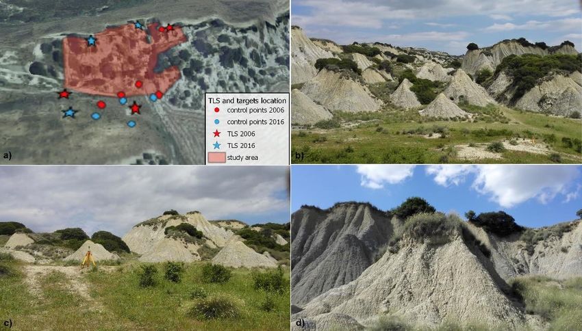
Land 2021, 10, 828                                                                                           2 of 17

                     then canalises in small gullies, forming residual conical domes of different morphologies
                     after the pipes’ roofs collapse [7,10,16]. In the lower topographic areas between domes, less
                     concentrated surface flows and deposition promote vegetation cover and micropediment
                     formation [12,13].
                           Even if the evolution of biancane is quite well known, their spatial continuous erosion
                     rates are not easy to assess [17]. These rates are very important in terms of sediment
                     (dis)connectivity on hillslopes and carbon dynamics [18,19]. In several studies, direct
                     erosion measurements were made with pins placed in slightly accessible areas where
                     piping was usually absent [8,20–23]. Indirect measurements can be calculated by com-
                     paring multi-temporal digital elevation models (DEMs) provided from digital stereopair
                     photograms [20,24] or, more recently, from lidar technology or unmanned aerial vehicle
                     (UAV) photogrammetry [25–29]. Comparative analyses between two or more DEMs of the
                     same area can highlight the slope areas affected by erosion or accumulation and provide an
                     estimation of the spatially distributed erosion rates [24,28,29]. The systematic and random
                     vertical errors in these studies have been assessed by measuring the elevation differences
                     between DEMs and ground control points (GCPs), and these errors are usually of values
                     on the order of centimetres [23,24,27,30], which are acceptable when considering the metric
                     ground level changes that occurred in the considered time span and the relatively large
                     size of the surveyed areas. However, the vertical errors are strictly linked to the DEM
                     resolutions. The choice of resolution is critical when using a DEM to study the spatial
                     patterns of these processes, since erosion and deposition are spatially heterogeneous across
                     hillslopes [31]. The DEM resolutions used in previous analyses ranges from a cell size of
                     5 m [20] or 2 m [24] to those ranging from 5 cm to 15 cm for studies using a terrestrial
                     laser scanner (TLS)- and structures from motion (SfM)-derived DEMs, respectively [27]. In
                     general, TLS provides more precise detection and quantification of changes, whereas SfM
                     DEMs are more appropriate to measure rates in wider areas [26–28].
                           Several studies have also analysed changes in hydrological catchments, quantifying
                     the accumulated or eroded volumes and detecting the morphological processes acting on
                     badlands [22,24,27]. In these studies, the factors acting on badland hillslopes, such as the
                     slope angle, orientation, vegetation, rain, and wind, were identified; in fact, badlands are
                     complex landscapes in which the interaction between different geomorphological processes
                     is present [32].
                           The correlation determined between erosion and the slope angle shows that the
                     steepest biancane sides experience major erosion due to the downward component of
                     splash and sheet erosion, which is dominated by gravity [33]. Additionally, exposure
                     affects the rate of erosion due to the dry and wet balances involved in sediment cohesion;
                     the presence of soil on the top contributes to the maintenance of steeper slope angles; and
                     vegetation can interfere with erosion processes [1]. Moreover, it has been suggested that
                     rills and pipe erosion produce similar quantities of sediment per unit of runoff discharge
                     under rainfall events [1,7]. Piccarreta et al. [14] showed how daily rainfall totals over
                     10 mm exceed the threshold for erosion occurrence, while rainfall amounts of 30 mm cause
                     severe rill erosion and mass movements on slopes. However, research on hydrological
                     and erosional contribution to badlands evolution has been conducted by rainfall field
                     simulation [34] and references therein]. Recently, some studies have pointed out how
                     the combined actions of rain and wind can accelerate erosion on slopes. The diversion of
                     raindrops from the vertical direction is directly proportional to the wind speed, up to a wind
                     speed of 6 m/s (which is a value within the moderate breeze on the Beaufort scale [35]).
                     For wind speeds greater than 6 m/s, the raindrop diversion angle slowly increases until the
                     wind speed reaches 10 m/s, and then remains constant [36]. Wind-driven rain (WDR) has
                     been investigated in several papers and is considered an important factor in soil erosion
                     and runoff generation, particularly under the combined conditions of heavy rainfall with
                     low to moderate winds [36–39]. According to Marzen et al. [38], WDR has a great impact
                     on runoff generation and is a crucial factor for natural hazard risk assessments, since it
                     can increase soil erosion. However, until now, all WDR studies have been carried out in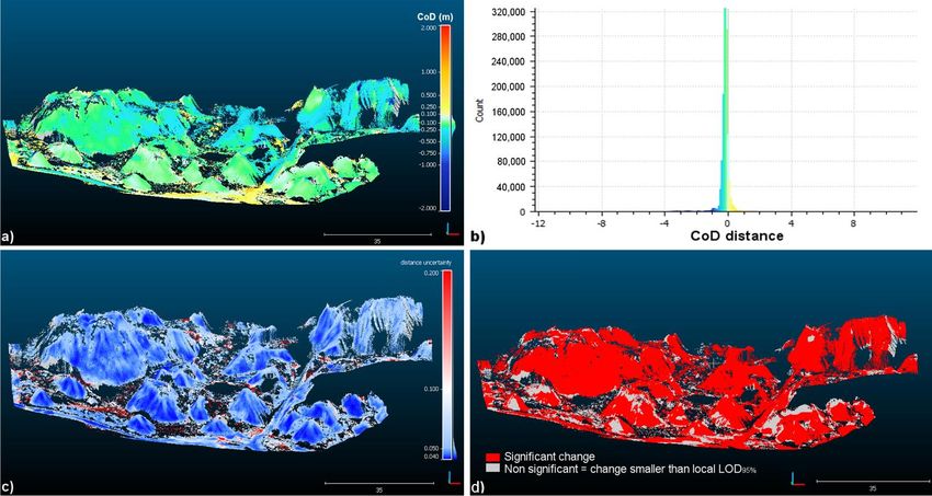
Land 2021, 10, x FOR PEER REVIEW 3 of 18
Land 2021, 10, 828 3 of 17
great impact on runoff generation and is a crucial factor for natural hazard risk assess-
ments, since it can increase soil erosion. However, until now, all WDR studies have been
carried out in laboratory experiments using wind tunnels, and it is difficult to assess the
laboratory experiments using wind tunnels, and it is difficult to assess the contribution of
contribution of WDR to slope erosion under field conditions also taking into account the
WDR to slope erosion under field conditions also taking into account the main direction of
main direction of surface wind in different weather types [40].
surface wind in different weather types [40].
We used multi-temporal surveys carried out by high-precision TLS technology to de-
We used multi-temporal surveys carried out by high-precision TLS technology to
tect where topographic changes occur on biancane hillslopes. The detailed 3D model com-
detect where topographic changes occur on biancane hillslopes. The detailed 3D model
parison led to assessment of the amount of changes, as erosion or deposition, and how the
comparison led to assessment of the amount of changes, as erosion or deposition, and how
influence of the morphological setting, of rainfall, and main direction of WDR can affect
the influence of the morphological setting, of rainfall, and main direction of WDR can affect
changes on the surface.
changes on the surface.
2.
2. Materials
Materials and
and Methods
Methods
2.1. Study
Study Area: Geological
Geological and
and Climate Data
The study area is located in the well-known badlands of the Basilicata region near
Aliano, Italy (Figure 1) on a south-facing hillslope of a monocline, and is approximately
10,000 m
10000 m22. .The
Thearea
areaisissituated
situatedbetween
betweenthethe central
central part
part of
of the
the Bradanic
Bradanic Trough
Trough and the
Lucanian Apennines,
Apennines,and andis is
in in
thethe
north-eastern areaarea
north-eastern of theofPlio-Pleistocene Sant’Arcangelo
the Plio-Pleistocene Sant’Ar-
Basin. The
cangelo Basin.outcropping succession
The outcropping ranges from
succession ranges 500 to 900
from 500mtothick [41,42]
900 m thick and is mainly
[41,42] and is
characterised by grey-blue marls, with rare beds of sands and shallow
mainly characterised by grey-blue marls, with rare beds of sands and shallow marine marine clays with
middle–high
clays plasticities.plasticities.
with middle–high The sediments include minerals
The sediments includewith highwith
minerals Na content
high Naminerals
content
with the tendency
minerals to disperse
with the tendency to rapidly
dispersewhen wetted
rapidly when [43].
wetted [43].
The study area was affected by the uplift of the eastern margin of the Apennine chain
during the
during the Upper
Upper Pliocene
Pliocene and
and Pleistocene
Pleistocene ages
ages [43].
[43]. Starting
Starting inin the
the Middle
Middle Pleistocene,
Pleistocene,
rivers incised deep valleys that extended perpendicularly to the coast due to continuous
rivers incised deep valleys that extended perpendicularly to the coast due to continuous
regional uplift,
regional uplift, climatic
climaticchanges,
changes,and andrelated sea-level
related sea-level movements
movements [44–47], whereas
[44–47], whereaserosion
ero-
affected the hillslopes, exposing highly erodible clayey bedrock.
sion affected the hillslopes, exposing highly erodible clayey bedrock.
Figure 1. Geological setting of the Aliano area; the studied hillslope area is shown by the red rectangle.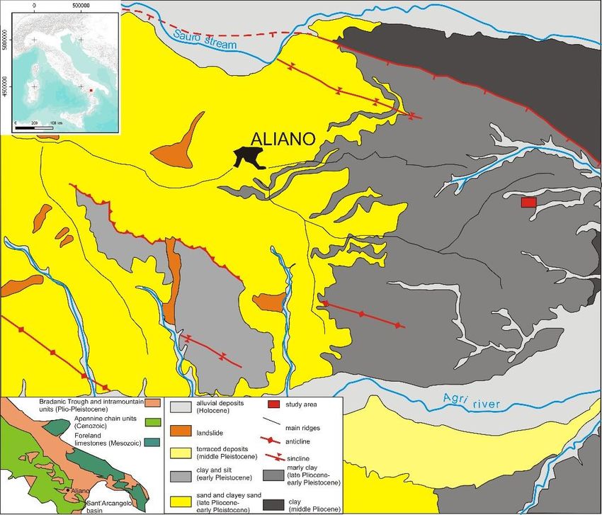
Land 2021, 10, x FOR PEER REVIEW 4 of 18
Land 2021, 10, 828 4 of 17
Figure 1. Geological setting of the Aliano area; the studied hillslope area is shown by the red rectangle.
In
Inthe
theAliano
Alianoarea,
area,the
thetopography
topographyis is characterised
characterisedbybya simple
a simpleNE-dipping
NE-dipping monoclinal
monocli-
landscape
nal landscape[13,14], withwith
[13,14], erosion
erosionfeatures common
features common to to
clayey-silty
clayey-silty terrain
terrainexposed
exposedtotothethe
south
south[48].
[48]. The
The seasonal
seasonal rainfall
rainfalldistribution,
distribution,highhighrelative
relativerelief,
relief,and
andnature
natureof ofthe
thebedrock
bedrock
have
have contributed
contributed to to creating
creating thethebiancane
biancanelandscape
landscape (Figure
(Figure2a,b).
2a,b). In
In the
the study
study area,
area,aa
high-density
high-density drainage network of small, inclined pipes in the middle part of theslope
drainage network of small, inclined pipes in the middle part of the slope
(Figure
(Figure2c)
2c)originates
originatesfrom
fromaasubsurface
subsurfaceflow flowthat
thatcauses
causescollapses,
collapses,andandthen
thenisolates
isolatescones
cones
at
atthe
thebases
basesofofthe
thehillslopes
hillslopes(Figure
(Figure2d),
2d),where
wherethetheoverland
overlandflows
flowsprevail
prevailandandthe
thecrust
crust
crumbles
crumblesin insmall
smallgullies
gulliesthat
thatcreate
createresidual
residualcones
cones[14].
[14].AArecent
recentstudy
study[15][15]showed
showedthatthat
the dome-shaped features are influenced by NW-SE strike-slip shear
the dome-shaped features are influenced by NW-SE strike-slip shear fractures and that fractures and that
structural
structural discontinuities
discontinuities within
within thethe claystones
claystones are
are the
the main
main factors
factors responsible
responsible forforthe
the
gravity-driven mass movements and erosion
gravity-driven mass movements and erosion processes. processes.
Figure2.
Figure 2. (a)
(a) 3D
3D view
view ofofthe
thestudy
studyarea
areaand
andlocation
locationofof
TLS and
TLS control
and points
control in both
points 2006
in both andand
2006
2016surveys;
2016 surveys; (b)
(b) the
the surveyed
surveyed biancana
biancana landscape
landscape characterised
characterised by
by isolated
isolateddomes
domesat atthe
themiddle
middle
and at the base of the slope; (c) dome-shaped features at the base of a slope, showing one of the
and at the base of the slope; (c) dome-shaped features at the base of a slope, showing one of the
highest-resolution control points (targets) used to overlap the scans; (d) a typical dome-shaped
highest-resolution control points (targets) used to overlap the scans; (d) a typical dome-shaped
feature with vegetation on its top; rills are visible on the slope.
feature with vegetation on its top; rills are visible on the slope.
This part of the Basilicata region enjoys the Mediterranean climate, characterised by
This part of the Basilicata region enjoys the Mediterranean climate, characterised by
warm, dry summers with a mean maximum summer temperature of approximately◦ 25
warm, dry summers with a mean maximum summer temperature of approximately 25 C,
°C, and temperate, wet winters with a mean minimum temperature of 9 °C. Here, the
and temperate, wet winters with a mean minimum temperature of 9 ◦ C. Here, the mean
mean annual
annual rainfallrainfall is between
is between 530 and 530 and
740 mm, 740with
mm,awith
heavy a heavy rain period
rain period from Novem-
from November to
ber to January [11], and then this area can be classified as semi-arid
January [11], and then this area can be classified as semi-arid biancana badlands [49]. biancana badlands
The
[49].follows
rain The rain follows
the the Mediterranean
Mediterranean rainfall
rainfall trend thattrend
showedthatashowed
general areduction
general reduction in
in the total
the total
annual annual precipitation,
precipitation, as well as as an well as an
increase in increase in the
the rainfall rainfall
intensity in intensity in the last
the last decades of
decades of the 20th century, followed by an increase in both the total
the 20th century, followed by an increase in both the total precipitation and daily rainfall precipitation and
daily rainfall
amounts sinceamounts
the beginningsince the
of thebeginning of the
21st century 21stFurthermore,
[50]. century [50].the Furthermore, the pre-
previous increases
vious increases in the lengths of the dry periods during winter and
in the lengths of the dry periods during winter and spring were followed by a decrease spring were followed
bythe
in a decrease
dry-spell inlengths
the dry-spell lengths in
in all seasons in all seasons
recent in recent
decades. decades.
In the study In theat
area, study area, at
the Aliano
the Aliano
gauge gauge
station, station, an
an analysis of analysis of pluviometric
pluviometric data shows data
an shows
annualan annual
mean mean precip-
precipitation of
itation of approximately
approximately 750 mm, with 750 mm, with precipitation
precipitation mainly concentrated
mainly concentrated betweenbetween
OctoberOcto-
and
ber and January.
January. An increase An increase
in rainfallin intensity
rainfall intensity
occurred occurred
between between
1955 and 1955 anddespite
2000, 2000, despite
a net
a net decrease in the total annual precipitation, highlighted by the increase
decrease in the total annual precipitation, highlighted by the increase in consecutive dry in consecutive
dry days
days anddecrease
and the the decrease in consecutive
in consecutive wet dayswet days recorded
recorded at Aliano
at Aliano [50]. [50].
2.2. TLS Survey and Data Processing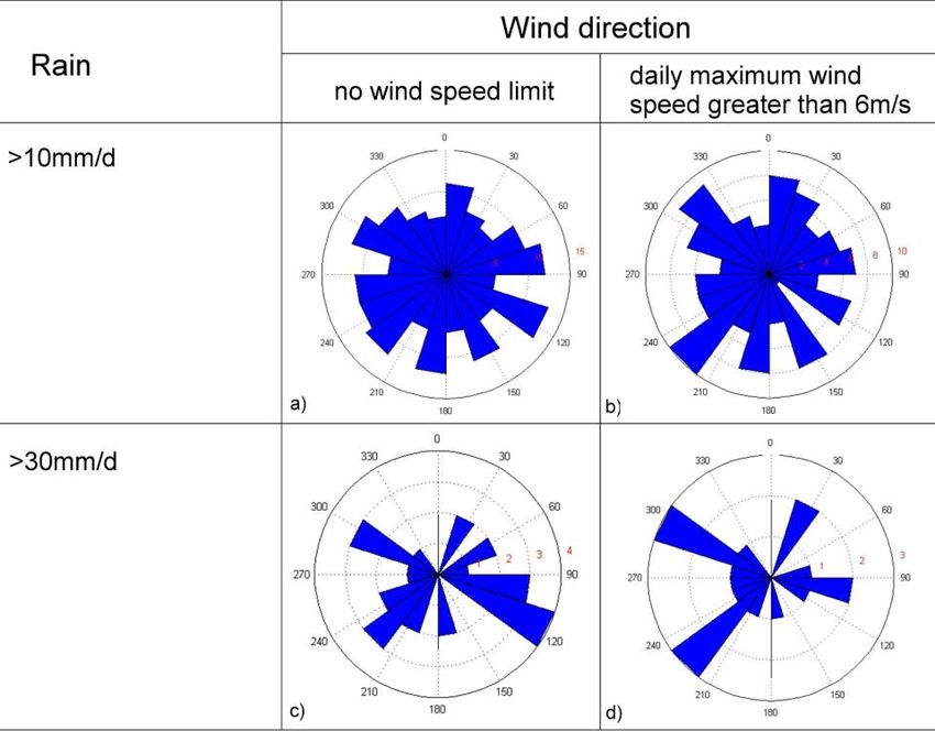
Land 2021, 10, 828                                                                                            5 of 17

                     2.2. TLS Survey and Data Processing
                           The lidar technology and the photogrammetry are non-contact survey methods avoid-
                     ing unnecessary disturbance to highly erodible badland surfaces, obtaining 3D models of
                     great accuracy and density [25]. The lidar technology is based on the principle of sending
                     out a laser pulse and observing the time it takes for the pulse to reflect off an object and
                     return to the instrument sensor. The distance range is combined with high-resolution
                     angular encoder measurements to provide the three-dimensional location of the observed
                     point [51]. A high-speed, high-accuracy Leica HDS 3000 terrestrial laser scanner was
                     used [52], and the result obtained was a point cloud.
                           TLS surveys of the Aliano badlands were conducted in 2006, between the 30th and 31st
                     of March, and on the 19th of May in 2016. In accordance with the topography of the study
                     area, the TLS was strategically positioned in several locations to cover, as much as possible,
                     the ground surface (Figure 2a). In fact, multiple scans at different locations were required to
                     capture the entire survey site because the scanner line-of-flight was obscured by domes and
                     brushes in one or more of the scan locations. We also chose these locations as a compromise
                     between the survey cover needs and the battery life. The scan resolutions ranged between
                     30 and 50 mm, both horizontally and vertically, to obtain the ground morphology. Each
                     scan had to contain the highest-resolution control points (targets, Figure 2c) of the previous
                     scan, thus providing overlap locations at which to join the scans into one single point cloud
                     representing the whole site.
                           The data processing, conducted with Cyclone© software [52], generated 3D point
                     clouds composed of millions of points according to the previously arranged spatial res-
                     olution; the positions of the overlapping targets were surveyed by differential GPS to
                     geo-reference the whole point cloud. We collected 5 scans in 2006 and 3 scans in 2016, and
                     we merged the scans of each year using a registration process. The RMSEs in the scan
                     registration were 0.002 m for the 2006 survey and 0.003 m for the 2016 survey.
                           Further data processing was performed using CloudCompare software version 2.10 [53].
                     The sparse vegetation on the ground surface was mostly removed by the filter tool (CANUPO)
                     based on user-defined ground identifications [54], while multi-temporal change detection
                     between the 2006 and 2016 point clouds was performed by the Multiscale Model to Model
                     Cloud Comparison (M3C2) plugin [55]. This algorithm produces a new point cloud that
                     shows the distance between the previous point clouds (CoD, cloud of difference) and al-
                     lows the assessment of data accuracy by showing the level of detection (LOD) at 95% and
                     the significant changes using 3D models. The LOD95% represents the spatially variable
                     confidence intervals of distance measurements and comes from the given combination of
                     different sources of uncertainties, such as the position uncertainty of the point clouds due to
                     instrument precision, the registration errors between point clouds, and the surface rough-
                     ness [30,55]. Hence, the measured distance was accurate where the change was greater
                     than the estimated errors in 95% of the cases and where the statistically significant changes
                     were visible on the point clouds, since the algorithm returned all these values stored in the
                     attribute table of the point cloud.
                           A further step in point cloud processing was made using a geographic information
                     system (GIS) to combine the biancane morphology with the multi-temporal changes and
                     to detect the locations where erosion and accumulation take place. Interpolating the 2016
                     biancane point cloud produced a DEM of the study area; by operating on this DEM, the
                     QGIS 3.2 tools allowed the slope angle and the exposure to be calculated. IDW interpolation
                     was applied on the CoD derived with the M3C2 plugin to create a raster of changes detected
                     on the slope. Finally, this CoD raster was combined with the both slope (45◦ ) and
                     exposure (315◦ < x < 45◦ ; 45◦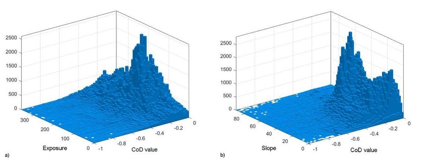
Land 2021, 10, 828                                                                                                 6 of 17

                     2.3. Rain and Wind Data
                          We collected rain and wind data from the ALSIA (Agenzia Lucana di Sviluppo e di
                     Innovazione in Agricoltura) station at Baderta Murgine (40.285929◦ N latitude, 16.316918◦
                     E longitude) near Aliano, approximately 2.8 km south-eastward from the study area. These
                     data cover the timespan between the first and last survey, and they were collected at both
                     daily and hourly rates.
                          The data were filtered accordingly with daily and hourly combined conditions of rain
                     and wind, and then displayed in rose diagrams.
                          We considered the wind direction of the events with daily rainfall amounts greater
                     than 30 mm, according to the method of Piccarreta et al. [14], to highlight on what sides and
                     how many times rainfall events caused severe rill erosion and mass movements. Moreover,
                     among these events, we selected those that occurred with a daily maximum wind speed
                     greater than 6 m/s, as this is an important threshold value for raindrop diversion in
                     WDR [36].
                          Similarly, we considered the wind direction during events with daily rainfall amounts
                     greater than 10 mm, the threshold for erosion occurrence according to Piccarreta et al. [14],
                     and we also investigated when these events occurred coupled with a daily maximum wind
                     speed greater than 6 m/s.
                          To support the contemporary occurrence of both intense rain and intense wind,
                     we also analysed the hourly data. According to the rainfall intensity classification [56]
                     (Table 1), rainfall rates between 2.5 and 10 mm/h are considered moderate, while rainfall
                     rates over 10 mm/h are considered heavy. We took into account the wind directions
                     during events with rainfall rates > 10 mm/h and those with rainfall rates > 6 mm/h, since
                     the latter is the rainfall intensity that causes significant erosion according to Foulds and
                     Warburton [57]. We then combined the rain events with rainfall rates > 10 mm/h and
                     >6 mm/h with contemporaneous occurrences of hourly mean wind speeds greater than
                     the threshold representing a gentle breeze on the Beaufort scale [35]. This value is 3.4 m/s
                     and also corresponds to the middle of the ascending stretch of the graph in Figure 3 in
                     Schmidt et al. [36], showing raindrop diversion from the vertical direction as a function
                     of wind speed. Since hourly mean wind speeds greater than 3.4 m/s rarely occur, we
                     also investigated rain events with rainfall rates > 10 mm/h and >6 mm/h that occurred
                     contemporaneously with maximum hourly wind speeds greater than 6 m/s, corresponding
                     to a moderate breeze, that is, the wind speed over which the splash and sheet erosion
                     process increases significantly [39].

                     Table 1. Rain intensity classifications according to the World Meteorological Organization, 2018.

                              Rain Range Intensity, i (mm/h)                             Classification
                                        < 2.5 mm/h                                           Slight
                                        2.5 ≤ i < 10                                       Moderate
                                        10 ≤ i < 50                                         Heavy
                                           i ≥ 50                                           Violent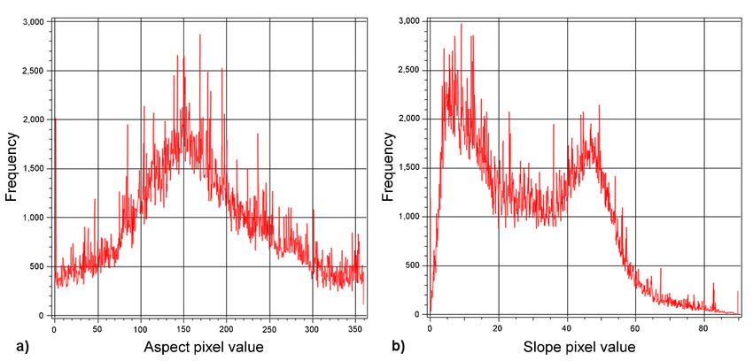
the slopes. The bulk of the values range between −0.43 m and −0.045 m, with a mean of
−0.23 m, resulting in a mean erosion rate of approximately 0.023 m/y (Figure 3b). The bulk
of positive values range from 0.04 m to 0.14 m. with a mean of 0.09 m, for an accumulation
Land 2021, 10, 828 rate of 0.009 m/y. Figure 3c shows the spatial distribution of the measurement uncertain-
7 of 17
ties. The uncertainty distribution is low almost everywhere and, as consequence, the
changes detected are significant on almost all the hillslope (Figure 3d).
Figure 3. Topographical
Figure 3. Topographicalchanges
changesdetected
detectedininthe
the biancane
biancane point
point clouds;
clouds; all all numeric
numeric values
values aremetres;
are in in metres; (a) south-side
(a) south-side view
view
of the CoD; (b) histogram showing the distribution of the values in (a); (c) uncertainty values shown as levelas
of the CoD; (b) histogram showing the distribution of the values in (a); (c) uncertainty values shown of level of
change
change detection at 95%; (d) statistically significant changes [55] derived from the combination of the CoD (a) and uncer-
detection at 95%; (d) statistically significant changes [55] derived from the combination of the CoD (a) and uncertainty (c).
tainty (c).
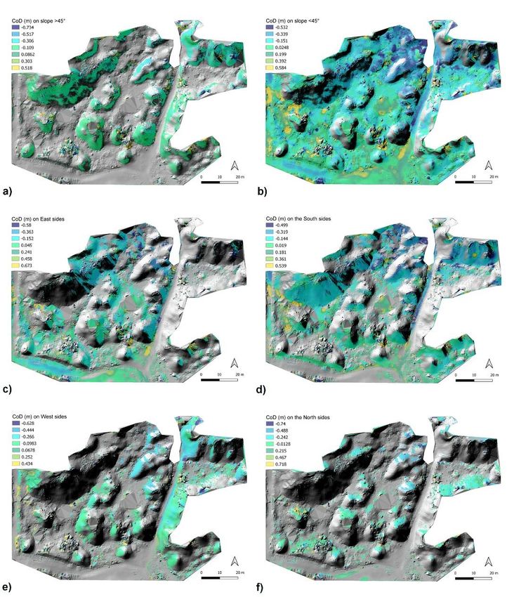
3. Results
Most ofDynamics:
3.1. Erosion the biancaneTLSsides areand
Survey steeper than 45°, with the steepest slope values greater
3D Model
than 60°, and most biancane are south- and southeast-oriented (Figures 4 and 5). The pro-
Erosion and accumulation are represented by negative and positive values, respec-
cessing of digital
tively, since these data allows
amounts us to measure
represent how the
the distances CoD the
between varies in the
points area,
in the both
2006 for
cloud
biancane sides with slope
and those in the 2016 cloud. angles greater and lower than 45° and according to the orienta-
tion of
Thetheresulting
sides (Figure
values5).are
Innegative
the CoD in raster
almostwith
theslope angles
entire studylower
area, than 45°, there
indicating are
erosion,
more pixels with positive values, indicating accumulation, than in the raster
while positive values showing accumulation are present only in the areas between biancane with slope
angles greaterpart
in the lower thanof45°.
the Even
studythough
area. Thethe erosion
majorityvalues
of the are
arealarger
has aon slope
the angle
tallestunder 45°
biancane
(Figure
located 5a,b),
in themost
upperof the
partpixels
of thewith
studythearea,
highest negative
while values,values
the erosion indicating erosion,
are lower oncor-
the
respond to slopes greater than 45°. The CoD rasters containing the east-
smallest biancane located in the lower part of the study area (Figure 3a). However, the and south-facing
sides
tallest(Figure
biancane 5c,d) showby
topped many more
shrubs pixels
shows witherosion
lower positivevalues
valuesonthan do the parts
the upper north-ofand
the
west-facing CoD rasters (Figure 5e,f). However, the CoD raster containing
slopes. The bulk of the values range between −0.43 m and −0.045 m, with a mean of north-oriented
sides
−0.23shows the highest
m, resulting negative
in a mean pixel
erosion values,
rate followed by0.023
of approximately the west-oriented
m/y (Figure 3b). CoDTheraster.
bulk
of positive values range from 0.04 m to 0.14 m. with a mean of 0.09 m, for an accumulation
rate of 0.009 m/y. Figure 3c shows the spatial distribution of the measurement uncertainties.
The uncertainty distribution is low almost everywhere and, as consequence, the changes
detected are significant on almost all the hillslope (Figure 3d).
Most of the biancane sides are steeper than 45◦ , with the steepest slope values greater
than 60◦ , and most biancane are south- and southeast-oriented (Figures 4 and 5). The
processing of digital data allows us to measure how the CoD varies in the area, both
for biancane sides with slope angles greater and lower than 45◦ and according to the
orientation of the sides (Figure 5). In the CoD raster with slope angles lower than 45◦ ,
there are more pixels with positive values, indicating accumulation, than in the raster
with slope angles greater than 45◦ . Even though the majority of the area has a slope angle
under 45◦ (Figure 5a,b), most of the pixels with the highest negative values, indicating
erosion, correspond to slopes greater than 45◦ . The CoD rasters containing the east- and
south-facing sides (Figure 5c,d) show many more pixels with positive values than do
the north- and west-facing CoD rasters (Figure 5e,f). However, the CoD raster containing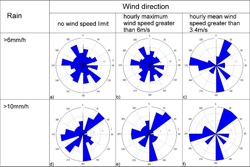
Land 2021, 10, 828 8 of 17
Land 2021, 10, x FOR PEER REVIEW 8 of 18
north-oriented sides shows the highest negative pixel values, followed by the west-oriented
CoD raster.
Figure4.
Figure 4. (a)
(a) Pixel
Pixel value
value frequency
frequency of
of the
the aspect
aspect raster
raster that
that shows
shows the
the exposure
exposure of ofbiancane
biancanerelief;
relief;the
thehighest
highestfrequency
frequencyisis
between90
between 90and
and220,220,that
thatis,
is,from
fromE-SE
E-SEtotoSW;
SW;(b)
(b)pixel
pixelvalue
valuefrequency
frequencyofofthe
theslope
sloperaster;
raster;although
althoughmostmostpixel
pixelvalues
valuesare
are
lowerthan
lower than40 40°, several pixels
◦ , several pixels have
havevalues
valuesover
over60
60°, and aa secondary
◦ , and secondary peak
peak is
is visible
visible around
aroundaavalue
valueof of50
50°.
◦.
Statistical analyses aided in determining how the erosion changed on the hillslope
sides. The statistical parameter distribution for each raster considered all the pixels that
ranged from the maximum value of approximately 8 m to the minimum value of approxi-
mately −6 m. These extreme values occurred due to noise still present in the point clouds
since it was very difficult to erase all the no-terrain points (e.g., vegetation). Table 2 reports
the statistical parameters of the six rasters processed according to the slope and aspect
distributions: differences are noticeable in the ranges of the most frequent pixel values and
in the quantities of these pixels, as noticeable by the % of area.
The mean, median, mode, and standard deviation values of the pixel distributions in
the CoD rasters on slopes over 45◦ confirm that the most negative values, corresponding to
higher erosion rates, are located on the steepest slopes.
The analysis of the pixel distribution of the CoD rasters selected according to the
exposure shows that the highest mean and median values are those of the west-exposure
raster, while the highest mode is that of the south-exposure raster. These results can be
related to the large quantity of pixels in the south-exposure raster, many of which have
positive values that lower both the mean and the median, although most of the pixels
consist of the highest negative values of the whole study area.
The mean pixel values of the raster with slope angles greater than 45◦ are the highest
among all rasters, even though the raster of the west exposure has a quite similar mean.
The great difference between these two rasters is in the mode value, which is higher for
the slope raster and indicates that the negative values are higher in the slope raster than
those in the west-exposure raster. Additionally, the mode value of the slope angle raster is
greater than that of the south-exposure raster, showing that the slope is an important factor
leading to erosion.
To highlight the correlations between erosion and exposure and between erosion
and slope angle, a bivariate histogram was calculated with only the negative CoD values
ranging between −1 m and 0 m (Figure 6); the greatest negative outlier values were not
taken into account since they probably occurred due to noise in the point clouds. Figure 6aLand 2021, 10, 828 9 of 17
shows that most of the pixels with low negative values are concentrated in the SW hillsides,
while the pixels with slightly higher negative values are located in the S and W hillsides of
Land 2021, 10, x FOR PEER REVIEW 9 of 18
biancane. Figure 6b shows that most of the pixels with negative values are concentrated on
◦
the steepest slopes, with angles around 60 , and a second peak is observed around slope
angles just beneath 20◦ .
Figure 5. The
Figure 5. CoD rasters
The CoD selected
rasters according
selected accordingtotothe
theside
side slope angles:(a)
slope angles: (a)greater
greater 45◦45°
than
than andand (b) lower
(b) lower 45◦ ; and
than than 45°;the
and the
side exposures facing:
side exposures (c) east,
facing: (d)(d)
(c) east, south, (e)(e)west,
south, west,and
and (f)
(f) north. TheCoD
north. The CoDvalues
valuesareare in metres.
in metres.
Statistical analyses aided in determining how the erosion changed on the hillslope
sides. The statistical parameter distribution for each raster considered all the pixels that
ranged from the maximum value of approximately 8 m to the minimum value of approx-
imately −6 m. These extreme values occurred due to noise still present in the point cloudsTable 2. Quantity (%) of study area occupied by pixel values and the statistical parameters computed for the pixel distri-
butions of the six rasters processed according to the slopes and exposures of biancane hillsides.
% of Area Mean Value Standard Deviation Median Mode (Distribution Peak)
Slope over 45° 23.52 −0.13567 0.40428 −0.14830 −0.16416
Land 2021, 10, 828 under 45°
Slope 76.37 −0.07019 0.34575 −0.10719 −0.1224 10 of 17
North sides (315° < x < 45°) 11.92 −0.10162 0.42931 −0.12574 −0.1375
East sides (45° < x < 135°) 28.1 −0.05777 0.35807 −0.09873 −0.102
South
Tablesides (135° < x(%)
2. Quantity < 225°) 39.8occupied
of study area −0.07755
by pixel values and0.35020
the statistical −0.12055
parameters computed−0.1586
for the pixel
distributions
West of the
sides (225° < xsix rasters processed
< 315°) 19.79 according to the slopes and0.33589
−0.13247 exposures of biancane hillsides.
−0.14227 −0.11915
Standard
% ofTo
Area Mean
highlight the Value
correlationsDeviation Median
between erosion Mode
and exposure and(Distribution Peak)and
between erosion
slope angle, a bivariate histogram was calculated with only the negative CoD values rang-
Slope over 45◦ 23.52 −0.13567 0.40428 −0.14830 −0.16416
ing between −1 m and 0 m (Figure 6); the greatest negative outlier values were not taken
Slope under 45◦ into76.37 −0.07019
account since occurred due−to
they probably0.34575 noise in the point−clouds.
0.10719 0.1224 Figure 6a
North sides (315◦ < x < 45◦ ) shows
11.92that most−0.10162
of the pixels with low negative
0.42931 values are concentrated
−0.12574 −0.1375 in the SW
East sides (45◦ < x < 135◦ ) hillsides,
28.1 while the pixels
−0.05777 with slightly higher
0.35807 negative
−0.09873 values are located in the S and W
−0.102
hillsides of biancane. Figure 6b shows that most of the pixels with negative values are
South sides (135◦ < x < 225◦ ) 39.8 −0.07755 0.35020 −0.12055 −0.1586
concentrated on the steepest slopes, with angles around 60°, and a second peak is ob-
West sides (225◦ < x < 315◦ ) 19.79 − 0.13247 0.33589
served around slope angles just beneath 20°. − 0.14227 − 0.11915
Figure6.6.Bivariate
Figure Bivariatehistograms
histogramscalculated byby
calculated comparing thethe
comparing CoD values
CoD with
values (a) the
with exposures
(a) the and and
exposures (b) the
(b) slope angles;
the slope the
angles;
the CoD
CoD valuesvalues ranged
ranged between
between −1 and
−1 and 0 metres.
0 metres.
3.2.
3.2.Rain
RainIntensity
Intensityand
andWDR
WDRCondition
Condition
Rain and wind data collected at the Baderta Murgine gauge station were filtered
to highlight the wind directions during different events. The climatic data collected in
the time lapse between the first and last TLS surveys show approximately 200 days with
daily rainfall amounts greater than 10 mm (Figure 7a), and only approximately 30 days
with daily rainfall amounts over 30 mm (Figure 7c). Figure 7a shows the wind directions
during events with daily rainfall amounts greater than 10 mm; heavy rainfall occurred
contemporarily with wind from all the main cardinal points. Events with a daily rainfall
amount greater than 30 mm mainly occurred with the ESE wind direction and with wind
coming from the NW and SW directions (Figure 7c).
Filtering the events of daily rainfall amounts greater than 10 mm and the daily maxi-
mum wind speeds greater than 6 m/s, we observe that there is a prevalent SW and NW
wind direction, but wind coming from the eastern side is also important (Figure 7b).
For the events of daily rainfall amounts greater than 30 mm with a daily maximum
wind speed greater than 6 m/s, we observe that there is a strong prevalence of the SW and
NW wind directions (Figure 7d).
The above analyses do not endorse the contemporary occurrence of both intense rain
and fast wind, which we investigated considering the hourly data. The number of events
with rainfall rates > 6 mm/h (moderate rain) was 159, and most of these events continued
for more than one hour, with wind that mainly came from the NW, W, SW, S, and SE
directions (Figure 8a). The number of events with recorded rainfall rates > 10 mm/h (heavy
rain) was 56; only in a few cases did heavy rainfall continue for two hours, and these events
were contemporary with winds coming from the NE, S, and W directions (Figure 8d). We
combined rainfall rates greater than 6 mm/h (Figure 8b,c) and greater than 10 mm/h
(Figure 8e,f) with both hourly maximum wind speeds greater than 6 m/s and hourly meanRain and wind data collected at the Baderta Murgine gauge station were filtered to
highlight the wind directions during different events. The climatic data collected in the
time lapse between the first and last TLS surveys show approximately 200 days with daily
Land 2021, 10, 828 rainfall amounts greater than 10 mm (Figure 7a), and only approximately 30 days with 11 of 17
daily rainfall amounts over 30 mm (Figure 7c). Figure 7a shows the wind directions during
events with daily rainfall amounts greater than 10 mm; heavy rainfall occurred contem-
porarily with wind from all the main cardinal points. Events with a daily rainfall amount
greaterspeeds
wind than 30 mm mainly
greater occurred
than with the
3.4 m/s. ForESE wind direction
rainfall and withthan
rates greater wind6coming
mm/h, we found that
from the NW and SW directions (Figure 7c).
the predominant wind directions were the NW, W, and SW directions
Filtering the events of daily rainfall amounts greater than 10 mm and the daily max-
for maximum hourly
wind speeds greater than 6 m/s (Figure 8b), and the S, W, and
imum wind speeds greater than 6 m/s, we observe that there is a prevalent SW and NW NE directions for hourly
mean wind speeds
wind direction, but windgreater
coming than 3.4eastern
from the m/s (Figure
side is also8c). The number
important of hours for which the
(Figure 7b).
For theofevents
first type eventofwas
dailyrecorded
rainfall amounts greater
was 133, thanthe
while 30 mm with aof
number daily maximum
hours for which the last type
wind speed greater than 6 m/s, we observe that there is a strong prevalence of the SW and
of event was recorded was only 21.
NW wind directions (Figure 7d).
Land 2021, 10, x FOR PEER REVIEW 12 of 18
hourly mean wind speeds greater than 3.4 m/s (Figure 8c). The number of hours for which
the first type of event was recorded was 133, while the number of hours for which the last
Figure 7. Wind directions during events with: (a) rainfall rates greater than 10 mm/d; (b) rainfall
Figure
type
rates of 7. Wind
event
greater was10
than directions
recorded
mm/d andwas during
dailyonly events
21.
maximum with:
wind (a) greater
speeds rainfall rates
than greater
6 m/s; than
(c) rainfall 10 mm/d; (b) rainfall
rates
rates For
greater rainfall
greater
than 30 thanrates
mm/d;10 greater
andmm/d than 10
andrates
(d) rainfall mm/h,
daily 50 events
maximum
greater were
wind
than 30 mm/d recorded,
speeds
and and the
greater wind
daily maximum predomi-
than 6 m/s; (c) rainfall rates
nant
speedswind directions
greater than 6 m/s.duringnumber
these of events were theinNE,
red. S, and W directions for hourly
greater than 30 mm/d;The and (d) rainfall days is shown
rates greater than 30 mm/d and daily maximum wind speeds
maximum wind speeds greater than 6 m/s (Figure 8e), while, during 13 events, the same
greaterThethan
directions 6 m/s.
were
above analysesThedonumber
also prevalent
notfor of days
hourly
endorse mean
the is shown in red.
wind speeds
contemporary greater than
occurrence 3.4 m/s
of both (Figure
intense rain
8f).
and fast wind, which we investigated considering the hourly data. The number of events
with rainfall rates > 6 mm/h (moderate rain) was 159, and most of these events continued
for more than one hour, with wind that mainly came from the NW, W, SW, S, and SE
directions (Figure 8a). The number of events with recorded rainfall rates > 10 mm/h (heavy
rain) was 56; only in a few cases did heavy rainfall continue for two hours, and these
events were contemporary with winds coming from the NE, S, and W directions (Figure
8d). We combined rainfall rates greater than 6 mm/h (Figure 8b,c) and greater than 10
mm/h (Figure 8e,f) with both hourly maximum wind speeds greater than 6 m/s and hourly
mean wind speeds greater than 3.4 m/s. For rainfall rates greater than 6 mm/h, we found
that the predominant wind directions were the NW, W, and SW directions for maximum
hourly wind speeds greater than 6 m/s (Figure 8b), and the S, W, and NE directions for
Figure 8. (a) Wind directions during hourly rainfall events greater than 6 mm; (b) wind directions
Figure 8. (a) Wind directions during hourly rainfall events greater than 6 mm; (b) wind directions
during rainfall rates greater than 6 mm/h and hourly maximum wind speeds greater than 6 m/s;
during rainfall rates
(c) wind directions duringgreater thangreater
rainfall rates 6 mm/hthan 6and
mm/h hourly maximum
and hourly wind
mean wind speeds greater than 6 m/s;
speeds
greater
(c) windthan 3.4 m/s; (d)during
directions wind directions
rainfallduring
rateshourly
greater rainfall
thanrates greaterand
6 mm/h than hourly
10 mm; (e) windwind speeds greater
mean
directions during rainfall rates greater than 10 mm/h and hourly maximum wind speeds greater
than
than 63.4 m/s;
m/s; (d)wind
and (f) wind directions
directions during
during rainfallhourly rainfall
rates greater thanrates greater
10 mm/h than mean
and hourly 10 mm; (e) wind directions
wind speeds
during greater
rainfall thangreater
rates 3.4 m/s. The
thannumber of hours
10 mm/h is shown
and hourlyin red.
maximum wind speeds greater than 6 m/s;
and (f) wind directions during rainfall rates greater than 10 mm/h and hourly mean wind speeds
Analysing the events, most of the time, rainfall amounts > 6 mm are characterised by
greater than
associated 3.4 m/s.
moderate to The
strongnumber
breezesof(Beaufort
hours isscale
shown in while
[35]), red. events with more in-
tense winds are less frequent (Figure 9a), and their quantities decrease with increasing
wind speeds. Hourly rainfall amounts >10 mm are frequently combined with strong
breezes, followed by winds from moderate to fresh breezes, and many events are linked
to near-gales or gales (Figure 9b).Land 2021, 10, 828 12 of 17
For rainfall rates greater than 10 mm/h, 50 events were recorded, and the predominant
wind directions during these events were the NE, S, and W directions for hourly maximum
wind speeds greater than 6 m/s (Figure 8e), while, during 13 events, the same directions
were also prevalent for hourly mean wind speeds greater than 3.4 m/s (Figure 8f).
Analysing the events, most of the time, rainfall amounts > 6 mm are characterised
by associated moderate to strong breezes (Beaufort scale [35]), while events with more
intense winds are less frequent (Figure 9a), and their quantities decrease with increasing
wind speeds. Hourly rainfall amounts >10 mm are frequently combined with strong
Land 2021, 10, x FOR PEER REVIEW breezes, followed by winds from moderate to fresh breezes, and many events are linked to
13 of 18
near-gales or gales (Figure 9b).
Figure 9.
9. (a)
(a)Frequencies
Frequenciesofofthe different
the wind
different windspeed classes
speed forfor
classes all events withwith
all events hourly rainfall
hourly amounts
rainfall greater
amounts than 6than
greater mm;6
the most frequent events are linked to wind speeds > 6 m/s andLand 2021, 10, 828 13 of 17
comparison of only two multi-temporal point clouds over a 10-year timespan is quite long
and is not a common timespan record to be surveyed by TLS. Nevertheless, thanks to a
continuous dataset of weather conditions recorded in the same time span, this approach
allowed us to appreciate how topographic changes occur on the biancane hillslope in
relation to the occurrence of all effective combinations of wind direction and rain intensity.
Our results show that the mean rate of erosion is approximately 0.023 m/y, which is
in accordance with the rates found in previous works (e.g., [10] and references therein),
and the mean rate of deposition is about 0.009 m/y, but topographic changes are not
evenly distributed on the hillslope and on dome sides. The sediment movement and
its budget in the biancane landscape is a consequence of the tectonic–lithological and
climatic setting [4,8,40,58–61], and changes in the erosion and deposition rates drive the
geomorphological evolution of the biancane reliefs.
On the other hand, the relief and exposure of the land surface can influence the erosion
and deposition rates in the biancana badlands. Over approximately 10 years, the study
area suffered a more intense erosion than deposition, as shown by the descriptive statistical
analysis on the CoD value. These topographical changes were not spatially uniform on the
biancane hillsides, since high slope angle and exposure played an important role in the
erosion of the slopes. A significant relationship between aspect and topographic change
was demonstrated by several authors [9,13,20,27]. In semi-arid badlands, the south facing
slopes show poor or no vegetation cover due to control of soil water availability, while the
north-facing slopes show higher vegetation cover [4,62–64]. In the study area, although
erosion was widespread on almost all domes, the analysis of the CoD raster showed that
all the southern (with the highest mode, Table 2) and western (with the highest median and
mean value, Table 2) sides of biancane suffer the most intense erosion, and sediments come
from steep bare south- and west-oriented slopes into lower topographic areas between
domes. Moreover, our analysis highlighted that erosion does not act evenly on the whole
hillside, but is more intense in the upper part of the surveyed area where the slopes were
greater than 45◦ . Combining these factors, we can assess that the steepest southwestern part
of the hillsides suffered the highest erosion. These results could be due to both the greater
insolation acting on the clay cohesion (exposure effect) and to the sediment movement
that acts on the slope under the control of gravity (slope angle effect). Although previous
study fixed the role of topography in the badlands slope gradient maintenance [9,13,17,25],
the CoD shows in detail how the sediments moved on hillslopes. The detailed survey
and the long timespan are also useful in order to suppose the way the runoff took place
under different rainfall conditions. In fact, our results confirm what was previously stated
under rainfall simulation [34]: sediment concentration in runoff is positively influenced by
slope angle, as sediment displacement is caused by splash and sheet erosion due to the
rainfall [37–39,63,65] that hits the sides of biancane. Our study shows that the necessary
conditions for intense rill erosion and mass movements on slopes (rain > 30 mm/d, [14])
rarely occur (approximately 30 days in 10 years) in the study area, but the conditions that
cause erosion (rain > 10 mm/d, [14]) are more frequent, occurring approximately 200 days
in the 10-year study period in these semi-arid badlands, where the mean annual rainfall is
between 530 and 740 mm [10]. As a consequence, the rainfall intensity over 10 mm/d is
critical in generating runoff in the area but, as several studies have shown [36–38,66,67],
wind is also an important factor in controlling runoff and soil erosion, since it contributes
to increasing rainfall action. Despite the important role of WDR, all previous studies were
performed in controlled environments (e.g., artificial rain and wind in wind tunnel) and no
relation was stated with erosion rate on biancana badlands. By combining the daily rain
with wind speed, our analysis highlights that the unstable weather linked to intense wind
comes from all E quadrants, from S and W. The more intense events are mostly linked to
western winds; they rarely occurred in the surveyed timespan, but their action on slopes
contributed anyway to the changes detected in this study on the exposed sides.
The daily values did not guarantee the simultaneous occurrence of wind and rainfall;
hence, we combine the rain and wind speed records of the same hours greater than theLand 2021, 10, 828 14 of 17
thresholds indicated in Section 2.3 in order to find the WDR. The rainfall with moderate to
strong breeze mostly affected dome sides facing W and S directions; when rainfall intensity
and wind speed increase, the most affected sides were those facing NE, S, and W. Finally, we
observed that rainfall > 6 mm/h was relatively frequent and was associated with winds of
moderate force coming from the western and southern sides. As the wind speed increased,
more intense events generally came from the NE direction and from the western directions,
and, despite their low frequency, the actions of these events could cause erosion on slopes
in any case, as shown by the CoD. In the study area, stronger events rarely occurred, and
the contribution to slope erosion was mainly due to the more frequent winds of moderate
forces, combined with moderate-to-heavy rainfall events. Since this WDR generally comes
from the southern directions (mainly SW and S), it is also combined with the insolation
(due to exposure) and gravity (due to slope angle) effects and contributes to an increase in
soil erosion on the south and southwestern facing hillslopes. However, we detected that,
in the case of more intense events, they acted also on slopes facing NE since WDR mainly
comes from this direction and potentially contributes to erosion on these biancane sides,
although insolation is less effective and particle cohesion is higher on these sides than those
on the other sides. The relation between the main WDR directions and the orientation and
slope of biancana hillslopes in the study area confirms how the local geomorphological
setting strictly affects the runoff distribution.
Even if our work was not focused on this topic, the role of scrubs and bushes on top
of some biancane is not negligeable in relation to both insolation and moderate or intense
WDR. We know that the roots retain sediments [1,2], but the bush foliage also acts as an
umbrella by shielding the upper part of slopes from both sun and WDR, partially reducing
erosion. In fact, on the domes that had bushes on top, we could observe a reduction in
erosion just beneath the shrubs, and this effect contributed to the steepness of the biancane
slopes (Figure 3a).
5. Conclusions
The multi-temporal high-resolution topographical survey of biancane-dominated hill-
sides conducted in this study measured the medium-term rates of erosion and deposition
over a 10-year timespan in this kind of landscape, and provided a detailed indication of
how the erosion and deposition rates were spatially distributed. A comparison of two
point clouds conducted by detecting the distances between homologous points led to a
survey of how erosion and sediment accumulation act on domes and in the areas between
them, allowing the assessment of the spatial distribution on erosion and deposition in a
complex topographic setting. We related different rates of sediment loss to different side
exposures and slope angles, obtaining the great influences of insolation, rainfall, and wind
on erosion and sediment movement. In fact, the sides that suffered the greatest erosion
were the southern and southwestern sides, clearly showing the relevance of insolation,
cracking, and scarce vegetation to sediment loss. Rain is an important factor in sediment
displacement, and its effect was directly dependent on the rainfall intensity and wind
direction. Our results confirmed the role of WDR in sediment erosion since raindrops and
soil particles are affected by the wind shear velocity. The most frequent WDR direction
corresponded to the exposure direction that suffered the greatest erosion. We found that
the most frequent moderate and heavy rains combined with moderate and heavy breezes
came from the S and SW directions, where the erosion was higher. We found that more
intense events acted on slopes facing NE, since WDR mainly came from this direction and
potentially contributed to erosion on these biancane sides, although insolation was less
effective and particle cohesion was higher than those on the other sides. The role of the
bushes on top of the domes slightly mitigated the effects of WDR.Land 2021, 10, 828 15 of 17
Author Contributions: Conceptualization, A.M.; methodology, A.M.; software, A.M.; validation,
A.M., V.D.S. and D.C.; formal analysis, A.M.; investigation, A.M. and D.C.; resources, D.C.; data cura-
tion, A.M. and V.D.S.; writing—original draft preparation, A.M.; writing—review and editing, V.D.S.
and D.C.; visualization, A.M.; supervision, D.C.; project administration, D.C.; funding acquisition,
D.C. All authors have read and agreed to the published version of the manuscript.
Funding: This research was funded by Program 2011–2013 PRIN (Response of morphoclimatic
system dynamics to global changes and related geomorphologic hazard; National co-ordinator: C.
Baroni; local Research Unit co-ordinators: G. Mastronuzzi).
Acknowledgments: We would like to thank the ALSIA (Agenzia Lucana di Sviluppo e di Innovazione
in Agricoltura) for the rain and wind data from Baderta Murgine station, and M. Zingaro for MATLAB
processing. We should like to thank the anonymous reviewers for their comments and suggestions
that improved the content of the manuscript.
Conflicts of Interest: The authors declare no conflict of interest.
References
1. Torri, D.; Santi, E.; Marignani, M.; Rossi, M.; Borselli, L.; Maccherini, S. The recurring cycles of biancana badlands: Erosion,
vegetation and human impact. Catena 2013, 106, 22–30. [CrossRef]
2. Bierbaß, P.; Wündsch, M.; Michalzik, B. The impact of vegetation on the stability of dispersive material forming biancane badlands
in Val d’Orcia, Tuscany, Central Italy. Catena 2014, 113, 260–266. [CrossRef]
3. Bryan, R.B.; Yair, A. Perspectives of studies of badland geomorphology. In Badland Geomorphology and Piping; Bryan, R., Yair, A.,
Eds.; Geo Books: Norwich, UK, 1982; pp. 1–12.
4. Calvo-Cases, A.; Harvey, A.M. Morphology and development of selected badlands in southeast Spain: Implications of climatic
change. Earth Surf. Process. Landf. 1996, 21, 725–735. [CrossRef]
5. Kuhn, N.; Yair, A. Spatial distribution of surface conditions and runoff generation in small arid watersheds, Zin Valley Badlands,
Israel. Geomorphology 2004, 57, 183–200. [CrossRef]
6. Cocco, S.; Brecciaroli, G.; Agnelli, A.; Weindorf, D.; Corti, G. Soil genesis and evolution on calanchi (badland-like landform) of
central Italy. Geomorphology 2015, 248, 33–46. [CrossRef]
7. Calzolari, C.; Ungaro, F. Geomorphic features of a badland (biancane) area (Central Italy) characterization, distribution and
quantitative spatial analysis. Catena 1998, 31, 237–256. [CrossRef]
8. Vergari, F.; Della Seta, M.; Del Monte, M.; Fredi, P.; Lupia Palmieri, E. Long- and short-term evolution of several Mediterranean
denudation hot spots: The role of rainfall variations and human impact. Geomorphology 2013, 183, 14–27. [CrossRef]
9. Pulice, I.; Di Leo, P.; Robustelli, G.; Scarciglia, F.; Cavalcante, F.; Belviso, C. Control of climate and local topography on dynamic
evolution of badland from southern Italy (Calabria). Catena 2013, 109, 83–95. [CrossRef]
10. Brandolini, P.; Pepe, G.; Capolongo, D.; Cappadonia, C.; Cevasco, A.; Conoscenti, C.; Marsico, A.; Vergari, F.; Del Monte, M.
Hillslope degradation in representative Italian areas: Just soil erosion risk or opportunity of development? Land Degrad. Dev.
2018, 29, 3050–3068. [CrossRef]
11. Alexander, D. Difference between “Calanchi” and “biancane” badlands in Italy. In Badland Geomorphology and Piping; Bryan, R.,
Yair, A., Eds.; Geo Books: Norwich, UK, 1982; pp. 71–88.
12. Torri, D.; Bryan, R.B. Micropiping processes and biancana evolution in southeast Tuscany, Italy. Geomorphology 1997, 20, 219–235.
[CrossRef]
13. Farifteh, J.; Soeters, R. Origin of calanchi and biancane in East Aliano, southern Italy. Geomorphology 2006, 77, 142–152. [CrossRef]
14. Piccarreta, M.; Faulkner, H.; Bentivenga, M.; Capolongo, D. The influence of physico-chemical material properties on erosion
processes in the badlands of Basilicata, Southern Italy. Geomorphology 2006, 81, 235–251. [CrossRef]
15. Bentivenga, M.; Agosta, F.; Palladino, G.; Piccarreta, M.; Prosser, G. Structural control on badland slope evolution: A case study
from the southern Apennines (Italy). Geomorphology 2021, 374, 107518. [CrossRef]
16. Torri, D.; Colica, A.; Rockwell, D. Preliminary study of the erosion mechanisms in a Biancana badland (Tuscany, Italy). Catena
1994, 23, 281–294. [CrossRef]
17. Cantón, Y.; Solé-Benet, A.; De Vente, J.; Boix-Fayos, C.; Calvo-Cases, A.; Asensio, C.; Puigdefábregas, J. A review of runoff
generation and soil erosion across scales in semiarid south-eastern Spain. J. Arid. Environ. 2011, 75, 1254–1261. [CrossRef]
18. Zingaro, M.; Refice, A.; Giachetta, E.; D’Addabbo, A.; Lovergine, F.; De Pasquale, V.; Pepe, G.; Brandolini, P.; Cevasco, A.;
Capolongo, D. Sediment mobility and connectivity in a catchment: A new mapping approach. Sci. Total. Environ. 2019, 672,
763–775. [CrossRef]
19. Zingaro, M.; Refice, A.; D’Addabbo, A.; Hostache, R.; Chini, M.; Capolongo, D. Experimental Application of Sediment Flow
Connectivity Index (SCI) in Flood Monitoring. Water 2020, 12, 1857. [CrossRef]
20. Ciccacci, S.; Galiano, M.; Roma, M.A.; Salvatore, M.C. Morphological analysis and erosion rate evaluation in badlands of
Radicofani area (Southern Tuscany—Italy). Catena 2008, 74, 87–97. [CrossRef]You can also read