Dispersion control in deformable microchannels
←
→
Page content transcription
If your browser does not render page correctly, please read the page content below
Journal manuscript No.
                                                        (will be inserted by the editor)

                                                    Dispersion control in deformable microchannels
                                                    Garam Lee1 · Alan Luner2 · Jeremy Marzuola2 · Daniel M. Harris1∗
arXiv:submit/3543196 [physics.flu-dyn] 6 Jan 2021

                                                    Received: date / Accepted: date

                                                    Abstract In fully-developed pressure-driven flow, the spread-     desirable to enhance dispersion (e.g. for mixing or reactions
                                                    ing of a dissolved solute is enhanced in the flow direction       [17,11]) or to minimize dispersion (e.g. for separations or
                                                    due to transverse velocity variations in a phenomenon now         chromatography [9,21]). In the present work, we develop a
                                                    commonly referred to as Taylor-Aris dispersion. It is well        novel technique for experimental control of dispersion on a
                                                    understood that the characteristics of the dispersion are sen-    single microchip via the continuous deformation of a rect-
                                                    sitive to the channel’s cross-sectional geometry. Here we         angular channel’s side wall. We first summarize the relevant
                                                    demonstrate a method for manipulation of dispersion in a          physical quantities associated with the problem in what fol-
                                                    single rectangular microchannel via controlled deformation        lows, also reviewed in detail within the 2006 review paper
                                                    of its upper wall. Using a rapidly prototyped multi-layer mi-     by Dutta et al. [10].
                                                    crochip, the channel wall is deformed by a controlled pres-           Consider steady, fully-developed, pressure-driven flow
                                                    sure source allowing us to characterize the dependence of         through a channel of uniform cross-section. At some instant
                                                    the dispersion on the deflection of the channel wall and over-    in time, a localized patch of a passive solute is introduced
                                                    all channel aspect ratio. For a given channel aspect ratio, an    into the flow and transported downstream and spreads due to
                                                    optimal deformation to minimize dispersion is found, con-         the effects of advection and diffusion. On long time scales,
                                                    sistent with prior numerical and theoretical predictions. Our     the solute assumes a Gaussian shape and grows diffusely
                                                    experimental measurements are also compared directly to           with an enhanced dispersion in the flow direction that can
                                                    numerical predictions using an idealized geometry.                be described by a Taylor-Aris dispersivity K

                                                    Keywords Taylor dispersion · Dispersion control ·
                                                    Deformable microchannel · Xurography                              K       1

                                                                                                                                        Uh
                                                                                                                                             2
                                                                                                                                                            1
                                                                                                                        = 1+                      f = 1+       Pe2 f           (1)
                                                    1 Introduction                                                    κ      210        κ                  210

                                                    When a localized patch of dissolved solute or other passive       where κ is the molecular diffusivity of the solute, U is the
                                                    tracer is introduced into a pressure-driven flow, it spreads      mean flow velocity, h is the characteristic channel height,
                                                    rapidly as it moves downstream through the subtle inter-          and f is a scale-free parameter that depends only on the
                                                    play of fluid advection and molecular diffusion [19,3]. This      cross-sectional shape of the channel. The Peclet number Pe =
                                                    phenomenon is now commonly referred to as Taylor-Aris             Uh/κ represents a ratio of the diffusive to advective time
                                                    dispersion and plays a critical role in many continuous mi-       scales. The second term on the right hand side of equation
                                                    crofluidic devices. Depending on the application, it may be       (1) represents the enhancement due to the presence of a non-
                                                                                                                      uniform fluid flow and becomes dominant for large Peclet
                                                    Daniel M. Harris
                                                                                                                      numbers.
                                                    E-mail: daniel harris3@brown.edu
                                                    1
                                                                                                                          Over the past several decades, there has been persistent
                                                     School of Engineering, Brown University, Providence, RI 02912,
                                                    USA.
                                                                                                                      interest in understanding the role of a microchannel’s cross-
                                                                                                                      sectional shape on its dispersion characteristics [7,8,10,1,
                                                    2 Department of Mathematics, University of North Carolina at      5,4,6,22,2]. As defined in equation (1), the cross-sectional
                                                    Chapel Hill, Chapel Hill, NC 27599, USA.                          shape defines the dispersion factor f through the boundary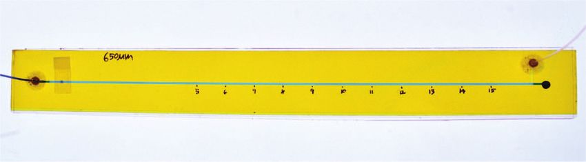
2                                                                                                                                Garam Lee1 et al.

    8                                                                         (a)                              (b) 2
                                                                                                                                δ = 0.6
    7                                                                                                                1.5         δ = 0.3
                                                                                             d                                    δ=0

                                                                                                               y h
    6                                                                                                                 1
                                                                                                                                δ = - 0.3
                                                                               h                                     0.5        δ = - 0.6
    5
                                                                                                                      0
    4                                                                                                                 -0.5         0           0.5
f

                                                                                                 w
                                                                                                                                  x w
    3                                                                         Fig. 2 Cross-sectional geometry. (a) Geometrical parameters of the
                                                                              channel with deformation of one wall. (b) The deflection parameter
    2                                                                         δ is defined as the ratio of the maximum deformation d over the orig-
                                                                              inal undeformed channel height h as δ = d/h. Positive δ represents
    1                                  w                                      outward deformation, and negative δ represents inward deformation.
                               h
    0
     1      2      3       4       5           6   7     8       9      10
                                           α                                  that a positive deflection parameter δ > 0 corresponds to an
Fig. 1 Dispersion factor f of a rectangular channel as a function of          outward bowing of the channel wall, a negative deflection
the channel’s aspect ratio α = w/h. The dispersion factor f is defined        parameter δ < 0 refers to an inward bowing, and δ = 0 is the
in equation (1). For reference, the case of infinite parallel plates corre-   undeformed rectangle. For all geometries studied, we define
sponds to a dispersion factor of f = 1.                                       h as the height of the undeformed rectangular geometry.
                                                                                  Dutta et al. [10] theoretically and numerically analyzed
conditions imposed on the flow problem. Physically, the dis-                  a similar “bowed” geometry (with a parabolic height profile
persion factor f is directly correlated to how “uniform” the                  on both top and bottom) and demonstrated that an optimal
velocity profile is across a particular channel’s cross-section.              bowing exists to minimize the dispersion coefficient for a
A more uniform flow field will tend to lead to lower disper-                  given channel aspect ratio. In particular, in the asymptotic
sion.                                                                         limit of |δ | ≪ 1 and α ≫ 1 it was predicted that this local
                                                                              minimum in the dispersion coefficient should occur at a de-
    The dispersion factor for a rectangular channel as a func-
                                                                              flection parameter of
tion of the aspect ratio α = w/h is shown in Figure 1. As
a point of reference, the case of two infinite parallel plates                               h    1.654
corresponds to a dispersion factor of f = 1. All rectangu-                    δo = −1.654      =−       .                                      (2)
                                                                                             w      α
lar geometries exceed this value due to the presence of the
vertical side walls. More recently, numerical and theoretical                 This asymptotic analysis can be applied to our idealized ge-
work have focused on how practical modifications to the tra-                  ometry as well, and yields the same result. According to
ditional rectangular channel geometry might reduce the dis-                   their result, the optimal deflection parameter is predicted to
persion factor [8,10,6]. One particular message that arises                   be inwards (δo < 0) with its magnitude decreasing with the
throughout these works is that by preferentially enlarging                    channel’s aspect ratio.
the cross-section near the vertical side walls, it is possible                    To the best of the authors’ knowledge, there remains no
to reduce the dispersion factor below the value for the pure                  experimental validation of the prediction of an optimal bow-
rectangle. This finding is rationalized physically in the re-                 ing. One recent experiment work relevant to the present dis-
view by Dutta et al. [10]: since a considerable amount of                     cussion was contributed by Miles et al. [16] who demon-
flow restriction (i.e. locally slower fluid flow) arises due to               strated the possibility of “flattening” the velocity profile in a
the presence of the vertical side walls, decreasing the lo-                   high-aspect ratio channel via bowing. However only a single
cal hydrodynamic resistance in these side regions leads to                    channel and deflection parameter were studied, and disper-
a more uniform velocity profile across the channel, thereby                   sion coefficients were not measured as part of this work.
reducing overall dispersion. Despite the numerical and the-                       The principal contributions of the present work are as
oretical progress in this direction, experimental results are                 follows. First, we develop and describe a novel and acces-
lacking.                                                                      sible rapid-prototyping fabrication technique which allows
    The present work focuses on a single class of cross-                      for continuous control of a microchannel’s cross-section by
sectional geometries shown in Figure 2. One wall of a rect-                   deforming one channel wall using a controlled external pres-
angular channel of overall aspect ratio α is deformed in a                    sure source. Dispersion experiments are then performed which
continuous curve with a peak deformation d. For this class                    demonstrate that the dispersion factor can be directly con-
of shapes, we expect the dispersion factor f to depend pre-                   trolled on a single microchip by nearly an order of magni-
dominantly on two dimensionless geometric quantities: the                     tude. Finally, the measured dispersion factors are shown to
base aspect ratio α and deflection parameter δ = d/h. Note                    be in good agreement with numerical predictions of an ide-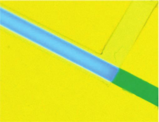
Dispersion control in deformable microchannels                                                                                            3

alized geometry and both exhibit a local minimum in the                0.8
dispersion factor at an optimal deflection parameter.                                                                                   10 2
                                                                       0.6
2 Numerical method and prediction
                                                                       0.4
The dispersion factor f can be computed as sequence of two
2D Poisson problems over the cross-sectional domain of the             0.2
channel. The theoretical formulation of this problem is re-
viewed in detail in prior work [10]. We parameterize the

                                                                   δ
                                                                         0
cross-sectional domain via a polygonal approximation made                                                                               10 1
with a fine discretization of the boundary curves. Then, we            -0.2

solve the corresponding Poisson problems through the MAT-
                                                                       -0.4
LAB PDE solver package by generating a reasonably fine
triangular mesh and the resulting finite-element stiffness ma-         -0.6
trices for both Dirichlet and Neumann boundary conditions.
From these, we are able to accurately integrate the numerical          -0.8                                                             100
                                                                               2           4            6         8          10
solution over the domain and compute the dispersion factor                                          α
 f for an arbitrary cross-sectional geometry.
                                                                   Fig. 3 Numerical calculation of the dispersion factor f as a function of
     In the present work, the cross-sectional geometry is de-      the aspect ratio α = w/h and deflection parameter δ . The white solid
fined by two non-dimensional parameters: the aspect ratio          line indicates a local minimum in the numerically determined disper-
α = w/h and the deflection parameter δ = d/h. For the pur-         sion factor corresponding to an “optimal” value δo for each aspect ratio.
                                                                   The dashed line represents an asymptotic analytical prediction for such
poses of the numerical calculation we assume the deformed
                                                                   a minimum (Eq. (2), [10]).
boundary to take the form of a parabola, as plotted in Fig-
ure 2(b). For small deformations, the numerical results are
found to be relatively insensitive to the exact functional form    are not readily accessible to all researchers. Furthermore
of the smooth upper curve.                                         the resources typically required for a single mold can limit
     The results of the numerical calculation are summarized       early-stage prototyping of channel designs.
in Figure 3. Of particular note, is that for each aspect ratio         For our work, we use a fabrication method that relies on
an optimal deflection parameter δo exists at which the dis-        a commercial desktop craft cutter. In this technique, some-
persion factor achieves a local minimum. These results are         times referred to as xurography, double-sided tape is cut into
consistent with the prior numerical work on bowed chan-            the designed channel shape by a commercial craft cutter and
nels wherein both the top and bottom walls are deformed            adhered to a transparent film and an acrylic sheet as an up-
symmetrically [10]. In the figure, we have also overlaid the       per and lower boundary of the channel. Using a craft cutter
asymptotic prediction for the optimal deflection parameter         for microchannel fabrication has been proposed before [23];
for a bowed channel (Eq. (2)) as predicted by Dutta [10]           however, the lack of the necessary wall smoothness and res-
which shows good agreement with our numerical predic-              olution for many microfluidic experiments have limited the
tions, particularly for large aspect ratios, the regime in which   implementation of the technique. Recent work [18] demon-
this theoretical result is derived.                                strated an optimized fabrication technique which achieved
     The numerical code used to perform these calculations         a surface roughness comparable to other leading fabrica-
is included as supplementary material. The results of the          tion techniques and can produce channels with dimensions
numerical study will be compared directly to experimental          as small as ∼ 100 µm. Ease of use of the devices and ex-
measurements in a following section.                               tremely short fabrication time makes prototyping of differ-
3 Experimental methods                                             ent channel designs significantly less costly. Furthermore,
                                                                   for controlled Taylor dispersion experiments, a channel with
3.1 Background                                                     a much longer length than typical microchannel sizes is re-
In the field of microfluidics, a commonly used technique to        quired to faithfully reach the Taylor-Aris dispersion regime.
fabricate a microchannel is soft lithography. Soft lithogra-       With the craft cutter used in this work we are able to cut a
phy uses a PDMS layer made by pouring an uncured PDMS              straight channel with length up to 20 cm (typically limited to
mixture on a patterned mold. This mold is generally a pro-         a few centimeters in soft lithography due to the wafer size)
duced by an optical lithography technique. The cured layer         and thus avoid the need for a serpentine channel [5,22].
of PDMS is peeled off of the mold and bonded to a substrate            Multi-layer soft lithography, which was first introduced
using plasma cleaning. Despite the wide applications and           by S.R. Quake and co-workers, is a technique to build an ac-
advantages of this technique, the required expensive equip-        tive microfluidic system containing microvalves and pumps
ment, highly trained personnel, and cleanroom environment          [20]. The system made from this technique consists of a flow
4                                                                                                                                Garam Lee1 et al.

(a)
                                                Air inlet                       (d)
              Dye hole

      Flow inlet                                        Flow outlet                                                                     Top

(b)                                                                                                                                     Flow layer

                               Flow channel
                                                                                                                                        Membrane
                               Air channel

                                                                                                                                        Air layer
(c)

                                                                                                                                        Base
                                Negave P             Posive P

(e)
                   Dye inlet                                                Air inlet

         Flow inlet                                                           Flow outlet

Fig. 4 Double-layer deformable microchip design. (a - c) Schematic and sectional views of the microchip. The flow channel includes an inlet and
an outlet while the air channel is a closed channel without an outlet. A flexible membrane placed between two channels is deformed via applied
pressure (or vacuum) in the air channel. (d) The complete chip is composed of five layers. Double-sided polyimide tape is used for the flow and the
air layer. The top and the base layer are made of transparent PET film and acrylic, respectively. (e) Fabricated microchip. The deformed channel
shape can be observed in the zoomed image; in this case, a positive pressure is applied to the air channel. Blue food dye was used here for ease of
visualization.

channel and an air channel stacked perpendicular to each                    a flexible membrane between the two channels. Fluids flow
other, and the two channels are separated by a thin PDMS                    along the straight flow channel and the air channel allows
membrane. When pressurized air is applied in the air chan-                  for control of the cross-sectional geometry of the flow by
nel, the membrane is deflected and obstructs the flow in the                changing the pressure in the channel as shown in Figure 4.
flow channel resulting in a flexible actuator or valve without                  For the flow layer and the air layer, double-sided poly-
the need for manufacturing or control processes with reso-                  imide tape (Bertech PPTDE-1) is used as the base material.
lution smaller than the scale of the channel itself.                        This tape is of total thickness 101.6 µm and is composed of
    Inspired by this multi-layer soft lithography technique, a              a 25.4 µm polyimide film with 38.1 µm of silicone adhesive
novel design of double-layer parallel channels is presented                 coating on each side. In the present work, we study three
within this work. Instead of placing the air channel and the                chips with different aspect ratios α = 3.0, 4.8, and 7.4 cor-
flow channel perpendicular to each other, the channels are                  responding to channel widths w of 300.4 µm, 488.6 µm, and
designed to be aligned parallel and exactly over top of one                 752.9 µm, respectively.
another. The parallel placement of two channels allows for
direct control of the channel’s cross-sectional shape by de-                     To form an upper boundary of the flow channel, 0.1 mm
forming one of the channel’s walls as depicted in Figure                    thick trasparent PET film (Grafix Dura-Lar Clear Acetate
4. The flow channel and the air channel are separated by a                  Alternative) is cut into the chip size with four holes: two
flexible membrane so that the membrane can bulge upward                     holes for the flow channel, one for the air channel, and one
and downward in a controlled manner in response to the ad-                  for introducing the tracer dye. A laser cutter (Universal Laser
justable static pressure in the air channel.                                Systems 4.60 with 30 Watt laser) is used to cut the PET
                                                                            film. The small hole on the top layer is sealed with tape,
3.2 Deformable microchip fabrication                                        and serves as direct access to the flow channel to introduce
Each deformable microchip incorporates two channels which                   the tracer dye. We observed that the experimental results
are placed parallel and directly over top of each other, with               are insensitive to minor variations to the details of the ini-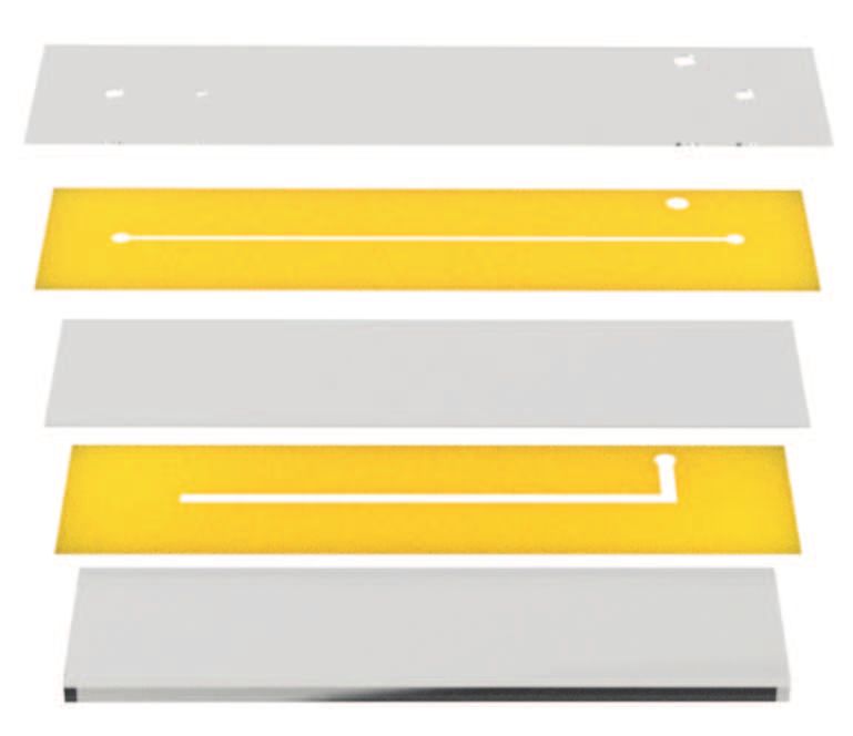
Dispersion control in deformable microchannels 5
(a) (e)
Light panel 250
200
Focusing rail
150
I
Microchip Camera 100
h = 101.6 µm
h = 203.2 µm
50 h = 304.8 µm
(b) (c) (d) h = 406.4 µm
h = 508.0 µm
0
0 0.05 0.1 0.15 0.2 0.25 0.3 0.35
1 mm Co h (g/m2)
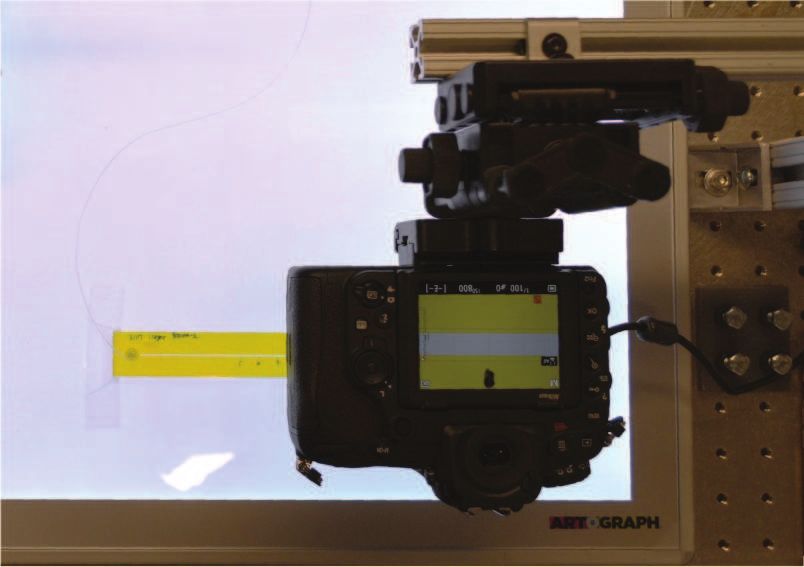
Fig. 5 Setup and image processing for bright-field imaging. (a) Optical setup. (b) Raw image, (c) decomposed B channel, (d) inverted result from
(c). (e) Intensity linearity validation. Channels of different thickness h (fabricated by changing the number of stacked double-sided tape layers) are
filled with dye solutions of known concentration Co and the intensity I of the inverted B channel is measured. The dashed line corresponds to a
linear fit of I = 137.3Co h + 37.4 up to an intensity of 160. The value Io = 37.4 corresponds to the value measured when no dye is present (Co = 0).
tial dye patch we achieved using this direct dye introduc- ily tunable cross-section. In this work, the entire experiment
tion method, as documented in prior work for rectangular is conducted within the flat region of 15 cm length, always
geometries [18]. at least 5 mm away from the ends of the membrane.
To construct the channels’ side walls, double-sided poly- In addition to the uniform pressure from the air channel,
imide tape is cut by a craft cutter (Silhouette Cameo 3) to the fluid movement in the flow channel generates a pres-
the desired channel design using the optimized protocol de- sure gradient along the channel length due to its viscosity. In
scribed in detail by Taylor & Harris [18]. Once the cut is this experiment, however, the pressure applied from the flow
complete, the channel negative and the circular part for the channel to the membrane can be safely neglected as the typi-
air inlet is removed. The cut flow layer is placed over the top cal pressure applied from the air channel required to deform
transparency and aligned with the inlet and the outlet holes the channel significantly is on the order of 10 kPa whereas
on the transparency. The flexible membrane is attached on the pressure drop along the flow channel is in the order of
the tape, and the cut air layer is sealed on the membrane en- 0.1 kPa (for the mean flow speeds of 1.0 mm/s used in this
suring that two channels share the same centerline. The min- work).
imum misalignment error that could be regularly achieved in
For a given membrane material, a larger air pressure is
this process was on the order of 15 µ m, although this step
could take several attempts and became easier with prac- needed to deform a narrower channel to the same deflec-
tice. A 3 mm thick optically clear acrylic sheet is attached tion parameter. Since a high pressure difference across the
membrane was observed to result in air passing through the
on the air layer as a chip base ensuring mechanical stability
membrane, pressure differences higher than 200 kPa were
and flatness. Capillary tubing (Cole Parmer PTFE #30 AWG
Thin wall tubing) and a tape gasket are adhered to the flow not used in our experiments. Considering the elastic behav-
and air inlets using an epoxy adhesive (PARTS Express 5 ior of the material and the applicable pressure range, plasti-
Minute Quik-cure Epoxy adhesive). cized PVC film (Stretch-tite premium plastic food wrap) is
used for α = 4.8 and 7.4 chips, and cross-linked silicon rub-
3.3 Membrane deformation ber film (Wacker ELASTOSIL Film 2030 250/50) is used
A long and narrow rectangular membrane deformed under a for the narrowest chip at α = 3.0.
uniform pressure loading takes an approximately 2D geom- To apply pressure to the air channel, an empty syringe
etry for the majority of its length. We will henceforth refer to (filled with air at atmospheric pressure) is used and con-
this region of the membrane with a uniform cross-sectional nected to a check valve. A pressure gauge is placed after the
shape as the ‘flat region.’ By avoiding the ends where 3D ef- check valve and connected to the air channel by a capillary
fects are observed (measured to be approximately 1 mm in tubing. Once the channel reaches a desired pressure by fill-
length in the present work), the long flat region allows us to ing or removing air in the system, the pressure is monitored
realize the experiment in a channel with a uniform but read- to ensure there is no pressure change during the experiment.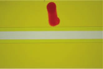
6                                                                                                                          Garam Lee1 et al.

3.4 Bright field imaging                                                                                             Pressure gauge

Fluorescence microscopy has been widely used in numer-                                                                          Pressurized air
                                                                                                      Check valve
ous fields of modern science including microfluidics due to
its superior sensitivity and the linear relationship between                                                         Camera

                                                                                                       e
                                                                                                        y
the concentration of a fluorophore and its fluorescence in-

                                                                                                           D
                                                                                     Water inflow
tensity [12,13]. However, the use of this technique requires
a special excitation source such as a mercury lamp and a          Syringe pump                                      Microchip
series of optical filters. While the system has many advan-
tages for measurements requiring high accuracy, a variety of      Fig. 6 Schematic of the overall experimental setup. The pressure in
                                                                  the air channel is controlled using an air filled syringe, and monitored
issues have to be considered [12]. One significant issue for
                                                                  with a pressure gauge. Fluid flow in the flow channel is introduced via
the present experiments is the photobleaching effect which        a syringe pump.
refers to a permanent loss of the ability for a fluorescent
chemical compound to fluoresce. This effect can add sig-
nificant error in the calibration between the intensity signal    read by the camera into a 2D map of the dye concentration
and the concentration field. Considering the apparent disad-      as it moves through the chip.
vantages of using fluorescence microscopy as well as overall      3.5 Dispersion experiment
higher equipment costs, bright field imaging on a flat light      The overall experimental setup is shown schematically in
panel was used in the present work.                               Figure 6. The fabricated microchip is connected to a glass
    The imaging setup is shown in Figure 5(a). The microflu-      syringe installed on a syringe pump (Harvard apparatus Stan-
dic chip is placed on 17 x 24 inch light panel (Artograph         dard Infuse-Withdraw Pump 11 Elite). A macro lens (Mi-
LightPad A950) to illuminate the microchip with uniform           takon Zhongyi 20 mm f/2 4.5x Super Macro Lens) is mounted
back lighting. To capture the intensity changes in the chan-      on the camera to image the channel. The resolution of the
nel, a camera (Nikon D500) is placed vertically over the chip     images taken in this setup is 1.04 µ m per pixel. The cam-
mounted on a focusing rail (Oben MFR4-5 Macro Focus-              era is centered 15 cm downstream from the dye inlet to en-
ing Rail) for precise camera alignment and focusing. To as-       sure that the solute patch reaches the long-time asymptotic
sess contrast between the channel region and the yellow tape      regime. Prior work [8] has shown that in rectangular chan-
representing the channel walls, the RGB channels of chan-         nel, the dispersivity approaches 95% of its long-time asymp-
nel images with and without flurescein dye were decom-            totic value after a time
posed and compared. Among the three channels, the Blue
(‘B’) channel demonstrated the best ability to distinguish             1 W2
                                                                  t≈        .                                                              (3)
the channel region. In fluorescence microscopy, higher in-             20 κ
tensity represents a higher concentration of dye molecules        For the mean flow velocity of 1.0 mm/s used throughout the
along the light path. In the contrary, in bright field imaging,   present work, the system is estimated to be in the asymptotic
a larger number of dye molecules block the light arriving to
the camera sensors which yields lower intensity. Hence, the
                                                                         1
raw B channel intensity values are first inverted by subtract-
ing them from the maximum possible intensity value 255 to
arrive a final map of the intensity I. This sequence of image          0.8

processing steps is shown for a sample channel in Figure
5(b-d).                                                                0.6
    Images processed as above were obtained to verify and
characterize a linear relationship between the measured in-            0.4
tensity and the product of the channel thickness and a pre-
scribed concentration of uniform dye solution in the chan-             0.2
nel. This product (height times concentration) is proportional
to the number of dye molecules within the cross-sectional
                                                                         0
area of the channel. As shown in Figure 5(e), a robust lin-
                                                                               130         140         150           160          170
ear regime was found up to an intensity value of 160, af-
                                                                                                         t (s)
ter which the relationship becomes nonlinear. By filling a
                                                                  Fig. 7 Curve fitting result for a sample experiment: α = 7.4 chip with
channel with a known concentration of fluorescein dye solu-
                                                                  δ = −0.36. The solid line is the best fit to equation (4) whereas the data
tion, we can now use this relationship to measure the height      points represent the results from six independent experimental trials.
profile of a deformed channel. Furthermore, in this linear        The Taylor-Aris dispersivity K is determined by the fit and can then be
regime, we can also faithfully translate the intensity signal     used to compute the dispersion factor f using equation (5).
Dispersion control in deformable microchannels 7
regime after around 5 cm downstream, using equation (3) as 200. Photos are taken with an interval of 1 s at the fixed posi-
a guide. tion 15 cm downstream from the dye hole. In post-processing,
First, the deformed profiles of the flow channel are mea- for each photo, an average intensity value is computed over
sured with various pressures applied to the air channel. By a cropped window spanning the entire width of the channel
filling up the flow channel with dye solution of a known and 100 pixels (∼ 0.1 mm) along its length. This allows for
concentration, the deformation profile is measured using the the determination of a representative intensity value I(t) as
linear relationship between the intensity and the height of the dye plug passes through the imaging location.
the channel. The cross-sectional area of the channel is then For each geometry, intensity profiles I(t) gathered from
calculated by numerically integrating the deformed channel six independent trials are overlaid, and the collected inten-
profile. After this measurement, the channel is flushed with sity time series are curve fit to a translating and diffusing
pure water to remove any residual dye solution. Gaussian distribution
Once the flow syringe and flow channel are filled with
water (and no air bubbles), the desired pressure is applied B
−(x0 − Ut)2
to the air channel. Any water exiting the outlet of the flow I(t) − Io = √ exp (4)
4π Kt 4Kt
channel is wicked away using a lint-free cloth.
Next a small droplet of fluorescein (HiMedia Laborato-
ries Fluorescein sodium salt) solution with a known molecu- as described in prior work [18]. The measurement position
lar diffusivity κ = 5.7 × 10⁻⁶ cm2 /s [2] is placed on the dye x0 and the average velocity U are known experimental pa-
hole using a syringe full of fluorescein dye solution. A solu- rameters and so only the dispersivity K and overall ampli-
tion of 2 g/L fluorescein dye is used which was confirmed to tude B is fit during this process. The overall amplitude B
remain in the linear measurement regime at the downstream varies between trials depending on the exact amount of dye
measurement location while also producing enough inten- introduced in the initial condition, but is otherwise irrele-
sity to maximize the signal to noise ratio in the intensity vant. An example of such a fit is shown in Figure 7. In this
signal. The dye hole is tape sealed again ensuring no bubble plot, each data set is normalized by the peak measured in-
is formed near the hole. The flow rate required to generate tensity value Imax so the curves can be superposed directly.
a flow velocity of U = 1.0 mm/s is set on the syringe pump Now knowing K for our trial, the dispersion factor f can thus
which is calculated based on the measured cross-sectional ultimately be calculated by inverting equation (1) yielding
area, as described previously.
With a mean flow velocity of 1.0 mm/s in these chips,
210 K
the corresponding Peclet number Pe is calculated to be ∼ f= −1 . (5)
Pe2 κ
(b)
(a)
18
y (µm)
100
16
14 0
0 100 200 300 400 500
12 x (µm)
(c)
δ = 0.45
10
0.29
f
8
0.15
6
0
4
-0.21
2 -0.38
0 -0.58
-0.6 -0.4 -0.2 0 0.2 0.4 0.6
δ t
Fig. 8 (a) Dispersion factor f versus deflection parameter δ in the α = 4.8 chip. Numerical predictions of dispersion factors are shown as a solid
black line, and experimental data are depicted with error bars drawn based on a standard multivariable error analysis [18]. (b) Measured cross-
section of deformed channel in experiment. (c) Intensity profile recorded at the fixed downstream position over time. The intensity is normalized
so that the maximum is the same brightness in all images. In reality, the wider distributions (corresponding to high dispersion) are significantly
more diluted.8 Garam Lee1 et al.
4 Results
Dispersivity of fluorescein dye in a deformed microchips
with three different aspect ratios was tested. The measured 0.8
widths of the flow channels are 300.4 µm, 488.6 µm and
0.6
752.9 µm, and the corresponding aspect ratios of the unde-
formed (δ = 0) chips are α =3.0, 4.8 and 7.4, respectively. 0.4
Figure 8(a) shows the measured dispersion factor f with
different deflection parameters δ in the α = 4.8 chip. The 0.2 10 1
experimental results are compared with corresponding nu- 0
δ
merical predictions, described in Section 2. Note that the
theoretical curve assumes an idealized geometry with a fixed -0.2
side wall height whereas in experiment the sidewalls also
-0.4
deform with the applied pressure, as can be seen in the mea-
sured channel geometries shown in Figure 8(b). Despite this -0.6
difference, the overall agreement is very good. In particular,
our results demonstrate that precise control of the disper- -0.8 10 0
2 4 6 8 10
sion is achievable in a single microchannel, with the disper- α
sion factor varying by nearly an order of magnitude between
geometries. Furthermore, the postulated presence of a local
Fig. 9 Experimental results of the dispersion factor f for three dif-
minimum in the dispersion coefficient has also been con- ferent microchips corresponding to α = 3.0, 4.8 and 7.4. Results are
firmed, and occurs at an inward bowing of around δ ≈ −0.4 overlaid on the numerical predictions. Each data point is derived from
for this microchip. six independent experimental trials. In this figure, f values obtained in
the simulation larger than 40 are depicted in the darkest color of the
Since we used a fixed mean flow velocity of 1.0 mm/s color map for improved contrast within the region of interest.
in all experiments, the trend in the dispersion factor is di-
rectly correlated to the length of the solute band in the flow
direction. Figure 8(c) shows the intensity profile over time comparison for the smallest aspect ratio chip when δ > 0,
at our measurement cross-section, corresponding to the data as can be seen in the upper left corner of Figure 9. A bet-
from Figure 8(a). Note that the figure is a time series of the ter quantitative agreement can be obtained by inputting the
intensity profile measured at a fixed spatial location, rather measured channel shapes directly into simulation, although
than an image of the solute distribution at a fixed moment in this does come at the cost of introducing a much larger set
time. of geometric parameters.
Figure 9 summarizes the results obtained from all three It is also possible that the comparison could be improved
chips fabricated in the present study. In general the compar- if the side wall height of the channel remained fixed, inde-
ison to the idealized theory is good, and each shows a local pendent of δ . In our experimental work we measured a clear
minimum in the dispersion factor for a particular level of deformation of the side walls that was correlated with the
inward bowing, as predicted numerically and in prior nu- applied pressure in the air channel. Different material se-
merical and theoretical work by Dutta et al. [10]. Some dis- lection for the flow channel or mechanical clamping of the
crepancies and limitations to the comparison do exist, and overall chip could potentially mitigate this effect.
will be detailed in the following section. Lastly, in long-time regime, the intensity profile of the
dye patch along the channel direction should converge to-
5 Discussion
wards a simple Gaussian distribution. However, we observed
While the overall trends of the numerics are well captured by notably skewed intensity profiles for cases with positive de-
our experimental results, some quantitative discrepancies do flection parameters δ > 0. The profile becomes increasingly
exist. In this section we will discuss some of the limitations skewed with larger deflection parameter δ and is likely an-
of the comparison and approach. other factor contributing to the quantitative discrepancy be-
The numerical values are calculated based on an ideal- tween the numerics (computed from long-time asymptotic
ized deformed channel shape that is defined by only two equations) and experiments. In designing the experiment,
parameters: the aspect ratio and the deflection parameter, the value computed from equation (3) was used as a criterion
where the upper arc of the bowed wall is assumed to be to determine the minimum distance the solute patch should
strictly parabolic. However, the channel geometry measured travel before measuring the intensity profile. However, this
from the experiment shows that this assumed geometry in guideline was only verified numerically in rectangular chan-
the numerical calculation is of course not a perfect repre- nels, which is evidently different for the deformed channel
sentation. This effect leads to the largest discrepancy in our shape considered in our work. Future theoretical and nu-Dispersion control in deformable microchannels 9
merical work might consider other methods to better quan- Acknowledgements DMH and GL gratefully acknowledge the finan-
tify the evolution of transient asymmetries in the distribution cial support of the Brown OVPR Salomon Award. JLM and AL were
supported in part by NSF CAREER Grant DMS-1352353 (2014-2020)
captured by higher moments (such as the skewness), as was
and NSF Applied Math Grant DMS-1909035 (2019-Present). Further-
recently documented for rectangular and elliptical geome- more, GL and DMH would like to acknowledge A. Taylor for support
tries [2]. and guidance with the craft-cutter technique, K. Dalnoki-Veress for
advice on membrane selection, and K. Breuer for use of his inverted
6 Conclusions microscope in preliminary experiments.
We have established an accessible method to control the dis- References
persion factor within a single multi-layer microchannel by 1. Ajdari, A., Bontoux, N., Stone, H.A.: Hydrodynamic dispersion in
deforming one of the channel walls in a controlled man- shallow microchannels: the effect of cross-sectional shape. Ana-
ner. The fabrication technique uses a commercial craft cutter lytical Chemistry 78(2), 387–392 (2006)
2. Aminian, M., Bernardi, F., Camassa, R., Harris, D.M., McLaugh-
which allows us to achieve this goal without relying on the lin, R.M.: How boundaries shape chemical delivery in microflu-
expensive equipment and facilities required by other com- idics. Science 354(6317), 1252–1256 (2016)
mon microfabrication techniques. The dispersion control tech- 3. Aris, R.: On the dispersion of a solute in a fluid flowing through
nique presented here does not rely on manufacturing or con- a tube. Proceedings of the Royal Society of London. Series A.
Mathematical and Physical Sciences 235(1200), 67–77 (1956)
trol process with resolution beyond that of the microchannel 4. Aubin, J., Prat, L., Xuereb, C., Gourdon, C.: Effect of microchan-
itself. To complete dispersion measurements in our custom nel aspect ratio on residence time distributions and the axial dis-
channels, we developed and validated a robust bright-field persion coefficient. Chemical Engineering and Processing: Pro-
cess Intensification 48(1), 554–559 (2009)
imaging setup using an artist’s tracing light pad and DSLR
5. Bontoux, N., Pépin, A., Chen, Y., Ajdari, A., Stone, H.A.: Exper-
camera, which further reduces the cost for performing such imental characterization of hydrodynamic dispersion in shallow
experiments. microchannels. Lab on a Chip 6(7), 930–935 (2006)
In our experimental measurements, we were able to iso- 6. Callewaert, M., De Malsche, W., Ottevaere, H., Thienpont, H.,
Desmet, G.: Assessment and numerical search for minimal taylor–
late the sensitive relationship between the dispersion factor aris dispersion in micro-machined channels of nearly rectangular
f and the deflection parameter δ on a single microchip. In cross-section. Journal of Chromatography A 1368, 70–81 (2014)
particular, for three microchannels of different aspect ratios, 7. Chatwin, P., Sullivan, P.J.: The effect of aspect ratio on longitudi-
nal diffusivity in rectangular channels. Journal of Fluid Mechanics
we experimentally verified the presence of a local minimum
120, 347–358 (1982)
in the dispersion factor as δ is varied continuously. This 8. Dutta, D., Leighton, D.T.: Dispersion reduction in pressure-driven
minimum value of f was found when the upper channel wall flow through microetched channels. Analytical chemistry 73(3),
was deformed inward by an amount which depends on the 504–513 (2001)
9. Dutta, D., Leighton, D.T.: Dispersion in large aspect ratio mi-
overall aspect ratio of the channel. crochannels for open-channel liquid chromatography. Analytical
Future work may include more detailed quantitative as- chemistry 75(1), 57–70 (2003)
sessment of the early time distributions in the experiment 10. Dutta, D., Ramachandran, A., Leighton, D.T.: Effect of channel
geometry on solute dispersion in pressure-driven microfluidic sys-
where significant skewness in the distribution is present [2].
tems. Microfluidics and Nanofluidics 2(4), 275–290 (2006)
Furthermore, the numerical code could be paired with an op- 11. Handique, K., Burns, M., Bhagat, A.A.S., Papautsky, I., Bandy-
timization scheme to identify other channel geometries with opadhyay, S., Goovaerts, R., Chen, C.f.: Micromixer based on tay-
even lower dispersion coefficients. lor dispersion. In: Journal of Physics: Conference Series, vol. 34,
pp. 136–141 (2006)
Given that the channel cross-section (and thus the dis- 12. Klimant, I., Huber, C., Liebsch, G., Neurauter, G., Stangelmayer,
persion factor) can now be controlled on a single chip, our A., Wolfbeis, O.S.: Dual lifetime referencing (dlr)—a new scheme
contributions open up potential for other exciting areas of for converting fluorescence intensity into a frequency-domain or
study. One area of interest might be in implementing real- time-domain information. In: New trends in fluorescence spec-
troscopy, pp. 257–274. Springer (2001)
time active control of dispersion processes in pressure-drive 13. Kuswandi, B., Huskens, J., Verboom, W., et al.: Optical sensing
flows. Alternatively, a similar device to ours could be used to systems for microfluidic devices: a review. Analytica chimica acta
study dispersion through a time-dependent channel geome- 601(2), 141–155 (2007)
14. Marbach, S., Alim, K.: Active control of dispersion within a chan-
try [14,15] with potential relevance to transport in biological
nel with flow and pulsating walls. Physical Review Fluids 4(11),
processes. 114202 (2019)
15. Marbach, S., Dean, D.S., Bocquet, L.: Transport and dispersion
Conflicts of interest across wiggling nanopores. Nature Physics 14(11), 1108–1113
(2018)
There are no conflicts to declare. 16. Miles, M., Bhattacharjee, B., Sridhar, N., Fajrial, A.K., Ball, K.,
Lee, Y.C., Stowell, M.H., Old, W.M., Ding, X.: Flattening of di-
Data availability luted species profile via passive geometry in a microfluidic device.
Micromachines 10(12), 839 (2019)
The datasets generated during and/or analysed during the
17. Nagy, K.D., Shen, B., Jamison, T.F., Jensen, K.F.: Mixing and dis-
current study are available from the corresponding author persion in small-scale flow systems. Organic Process Research &
on reasonable request. Development 16(5), 976–981 (2012)10 Garam Lee1 et al.
18. Taylor, A.W., Harris, D.M.: Optimized commercial desktop cutter 21. Westerbeek, E.Y., Bomer, J.G., Olthuis, W., Eijkel, J.C.,
technique for rapid-prototyping of microfluidic devices and ap- De Malsche, W.: Reduction of taylor–aris dispersion by lateral
plication to taylor dispersion. Review of Scientific Instruments mixing for chromatographic applications. Lab on a Chip 20(21),
90(11), 116102 (2019) 3938–3947 (2020)
19. Taylor, G.I.: Dispersion of soluble matter in solvent flowing slowly 22. Yan, X., Liu, M., Zhang, J., Zhu, H., Li, Y., Liang, K.: On-
through a tube. Proceedings of the Royal Society of London. Se- chip investigation of the hydrodynamic dispersion in rectangular
ries A. Mathematical and Physical Sciences 219(1137), 186–203 microchannels. Microfluidics and Nanofluidics 19(2), 435–445
(1953) (2015)
20. Unger, M.A., Chou, H.P., Thorsen, T., Scherer, A., Quake, S.R.: 23. Yuen, P.K., Goral, V.N.: Low-cost rapid prototyping of flexible
Monolithic microfabricated valves and pumps by multilayer soft microfluidic devices using a desktop digital craft cutter. Lab on a
lithography. Science 288(5463), 113–116 (2000) Chip 10(3), 384–387 (2010)You can also read