Diurnal and seasonal variability of CO2 and CH4 concentration in a semi urban environment of western India - Nature
←
→
Page content transcription
If your browser does not render page correctly, please read the page content below
www.nature.com/scientificreports
OPEN Diurnal and seasonal variability
of CO2 and CH4 concentration
in a semi‑urban environment
of western India
Abirlal Metya1,2, Amey Datye1, Supriyo Chakraborty1,2*, Yogesh K. Tiwari1, Dipankar Sarma1,
Abhijit Bora3 & Nirmali Gogoi3
Amongst all the anthropogenically produced greenhouse gases (GHGs), carbon dioxide (CO2) and
methane (CH4) are the most important, owing to their maximum contribution to the net radiative
forcing of the Earth. India is undergoing rapid economic development, where fossil fuel emissions
have increased drastically in the last three decades. Apart from the anthropogenic activities, the GHGs
dynamics in India are governed by the biospheric process and monsoon circulation; however, these
aspects are not well addressed yet. Towards this, we have measured CO2 and CH4 concentration at
Sinhagad, located on the Western Ghats in peninsular India. The average concentrations of CO2 and
CH4 observed during the study period are 406.05 ± 6.36 and 1.97 ± 0.07 ppm (µ ± 1σ), respectively. They
also exhibit significant seasonal variabilities at this site. CH4 (CO2) attains its minimum concentration
during monsoon (post-monsoon), whereas CO2 (CH4) reaches its maximum concentration during pre-
monsoon (post-monsoon). CO2 poses significant diurnal variations in monsoon and post-monsoon.
However, CH4 exhibits a dual-peak like pattern in pre-monsoon. The study suggests that the GHG
dynamics in the western region of India are significantly influenced by monsoon circulation, especially
during the summer season.
Carbon dioxide (CO2) is one of the minor (~ 0.4% of all gaseous species) constituents of the atmosphere. Still, it
plays the most significant role in the radiation balance of the planet among the species produced anthropogeni-
cally. CO2 contributes 73% of all positive radiative forcing of the Earth’s environment since the pre-industrial era,
circa 1750s1,2. CO2 is continuously being exchanged between the terrestrial biosphere, ocean, and the atmosphere3
and maintained a more or less steady-state, until about 1750. The balance in C O2 is being perturbed due to the
anthropogenic emission of CO2 and its feedback with the global climate change since the industrialisation4. The
atmospheric concentration of C O2 has progressively increased since the beginning of the industrialisation, from
280 ppm (in 1700) to a current level of more than 410 ppm. About one-fourth of the CO2 emissions from the
anthropogenic activities (fossil-fuel consumption, cement production, and land cover land-use changes) have
been absorbed by the ocean and another one fourth by the terrestrial biosphere during the 2000s1,5. The exchange
of carbon among the various reservoirs is controlled by complex biogeochemical processes and takes place on
various timescales6. A better understanding of the carbon exchange process, especially on a short temporal and
spatial timescale, is necessary to have a better estimate of the carbon b udget7,8. This requires a robust network of
continuous monitoring of C O2 concentration and determining its fluxes from different reservoirs4,9–11.
Methane (CH4) is the second-largest contributor, among the anthropogenically produced species, to global
warming with a positive radiative forcing of about 0.48 ± 0.05 W m−22. The pre-industrial C H4 concentration was
estimated to be 700 ppb, but increased anthropogenic activities have resulted in a steady increase of atmospheric
CH4, up to 1803 ppb in 2 01112,13. Apart from being a potent greenhouse gas, CH4 plays an active role in tropo-
spheric chemistry. C H4 is the main contributor to the increase in stratospheric water vapour, following the loss
by reaction with OH radical14. The water vapour variation in the upper troposphere and lower stratosphere is
highly significant due to its impact on global warming. C H4 emissions from anthropogenic sources in India have
increased from 18.85 to 20.56 Tg year−1 from 1985 to 200815. Unlike CO2, methane has a relatively short lifetime
of approximately 10 years16. Thus, in comparison with CO2, CH4 can attain a steady-state condition and start to
1
Indian Institute of Tropical Meteorology, MoES, Pune 411008, India. 2Department of Atmospheric and Space
Sciences, Savitribai Phule Pune University, Pune 411007, India. 3Department of Environmental Science, Tezpur
Central University, Tezpur, India. *email: supriyoc@gmail.com
Scientific Reports | (2021) 11:2931 | https://doi.org/10.1038/s41598-021-82321-1 1
Vol.:(0123456789)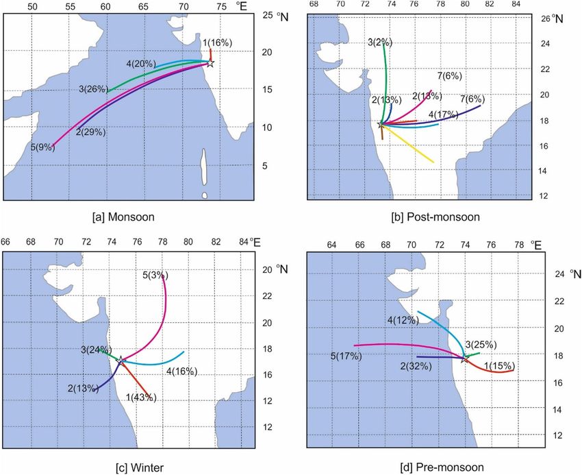
www.nature.com/scientificreports/
decrease reasonably fast if emissions are stabilised or reduced. However, increased emission of C H4, mainly due
to human activities, could perturb the equilibrium state. The source and sink mechanism of C H4 is complex, and
their pathways remain poorly constrained. Apart from a few mid-to-upper tropospheric observations of CH4
by satellite remote sensing, its surface monitoring over the Indian subcontinent is sparse. Hence, the key drivers
for its diurnal or seasonal scale variability are not well understood. The seasonal variation of CH4 over different
parts of India can be attributed to the complex interaction between surface emissions and convective transport
during monsoon as well as monsoon c irculation17,18. For example, the eastern Himalayan station Darjeeling
captures episodes of higher CH4 concentrations throughout the year19. A north-western Himalayan station Hanle
experiences high values during the summer monsoon season, while Pondicherry, located on the eastern coast
of India, and Port Blair, situated on an island in the Bay of Bengal, show comparatively lower values18. During
June–September, CH4 maxima at Hanle is likely due to enhanced biogenic emission from wetlands and rice
paddies. Also, deep convection associated with monsoon mixes surface emission to mid-to-upper troposphere
enhances the C H4 concentration at Hanle. Moreover, the elevated C H4 is also found in 8–12 km over a vast region
50°–80° E and south of 40° N during the CARIBIC (Civil Aircraft for the Regular Investigation of the Atmosphere
Based on an Instrument Container) aircraft observations20. Minimum CH4 at Pondicherry and Port Blair during
the monsoon season is associated with transportation of southern hemispheric C H4-depleted air at low altitudes
and high rates of OH o xidation18. The large scale observational network is required for understanding the spatial
and temporal variations in CH4 over India.
India is one of the largest and fastest-growing economies in South Asia and is a significant contributor to CO2
emissions in this region. Observations of diurnal and seasonal variations in the contribution of anthropogenic
and biogenic sources of CO2 and CH4 are well documented from many urban stations in Europe and the USA, but
only a few cases are documented in the Asian r egion21–23. Tiwari et al.24 have shown that CO2 variability during
winter months (seasonal amplitude) is higher (approx. double) than the summer months at a surface observa-
tional site in India. The monitoring was based on flask samples at the weekly interval, but no data is available
yet at higher temporal resolution. The short-term variations, such as on diurnal scale, capture the signature of
the photosynthesis process, respiration, and anthropogenic emission on the observed variability of atmospheric
CO2. Hence, it is interesting to identify the time-varying characteristics of CO2 and C H4 concentrations and the
probable causes, which characterise the variability in different time scales over peninsular India.
In view of the above, continuous measurement of C O2 and C H4 have been carried out from July-2014 to
November-2015 from Sinhagad, a Western Ghat site, using a highly sensitive laser-based technique. These meas-
urements are utilised for studying the temporal variations (diurnal and seasonal) of both the gases and identifying
the key drivers of such variations, especially the effect of monsoon circulation. The effects of meteorology as well
as vegetation dynamics on C O2 and CH4 concentration on different time scales are also investigated.
Study area
The study area (Sinhagad; denoted as sng: 18° 21′ N, 73° 45′ E, 1600 m above msl) is a semi-urban location in
the Western Ghats, India. This region is positioned at a distance of 30 km south-west from the city of Pune and
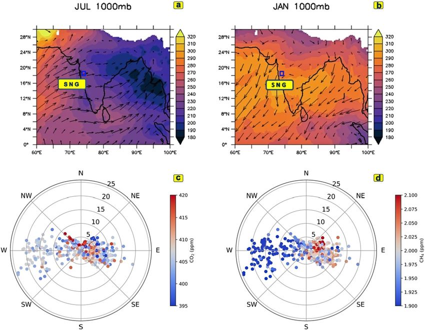
200 km east from the coastline of the Arabian Sea in Maharashtra, India. The basic climatology is presented in
Fig. 1. The outgoing longwave radiations (OLR), on a monthly scale for the summer and winter seasons, are
shown in Fig. 1a,b, respectively. The corresponding circulations are depicted by arrows. The windrose diagrams
for CO2 and CH4 are also shown (Fig. 1c,d).
Results
Seasonal variation of CO2 and CH4. Figure 2a,c shows the monthly mean and standard deviation
(SD; shaded region) of C O2 and C H4 concentrations, respectively. The annual mean concentration of C O2 is
406.05 ± 6.36 (µ ± 1σ) ppm. CO2 is maximum (427.2) in May-2015 and a minimum (399) in September-2014.
This leads to a seasonal amplitude of ~ 28 ppm. A comparison of the seasonal amplitude of other sites, global
(Seychelles-sey, Mauna Loa-mlo), and Indian sites (Kaziranga-knp, Ahmedabad-amd, Shadnagar-sad, Cabo de
Rama-cri), are shown in Fig. 2b. sey and mlo data are taken from ESRL-NOAA, knp data is obtained under
Metflux India25 project. amd and sad seasonality are taken from Chandra et al.22 and Sreenivas et al.26, cri data is
taken from World Data Centre for Greenhouse Gases (WDCGG). The global sites sey and mlo are mostly oce-
anic, hence possess smaller seasonal variation. In contrast, knp is a forest site of north-east India. It shows a larger
seasonality of ~ 25 ppm, with a minimum during pre-monsoon and post-monsoon (Fig. 2a). Ahmedabad is an
urban site in western India and has a CO2 seasonality of 26 ppm. Shadnagar is a semi-urban site in central India
with seasonality of 16 ppm. cri is a coastal region on the west coast of India. The mean seasonal amplitude of cri
is 20 ppm with a minimum in monsoon and maximum in February–March. Among all these sites, sng shows
maximum seasonal amplitude with pre-monsoon maximum and post-monsoon minima. Mean values of CO2
for different seasons are 403.34 ± 5.71, 402.87 ± 6.03, 409.72 ± 4.33, 417.06 ± 5.11 ppm during the monsoon, post-
monsoon, winter, and pre-monsoon, respectively. Mean C O2 increases about 6.85 ppm from post-monsoon to
winter and again increases about 7.34 ppm from winter to pre-monsoon.
The annual mean value of CH4 over the study region is 1.97 ± 0.07 (µ ± 1σ) ppm. C H4 concentration is mini-
mum (1.863 ppm) in July-2014 and maximum (2.037 ppm) in October-2014 (Fig. 2c). The seasonal pattern over
cri is very similar to the sng. The sng CH4 shows 2.29 times and 3.62 times more seasonality than global sites sey
and mlo (Fig. 2d). Whereas sad shows more seasonal amplitude of ~ 240 ppb than sng (~ 174 ppb). While cri
seasonal amplitude, 168 ppb, is very close to sng seasonal amplitude, 174 ppb. The average values of C H4 in dif-
ferent seasons are 1.903 ± 0.0412, 2.024 ± 0.0567, 1.995 ± 0.0629, 1.966 ± 0.0466 ppm in monsoon, post-monsoon,
winter, and pre-monsoon, respectively.
Scientific Reports | (2021) 11:2931 | https://doi.org/10.1038/s41598-021-82321-1 2
Vol:.(1234567890)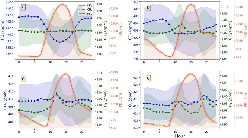
www.nature.com/scientificreports/
Figure 1. The outgoing longwave radiation on a monthly scale (shaded) at the surface (1000 mb) during (a)
July (average of 2014–2015) and (b) January (2015). Arrows indicate wind vectors. A blue rectangle marks
station Sinhagad. The wind rose diagram for (c) CO2 and (d) CH4 are also shown.
Influence of large scale circulation. To understand the large-scale meteorological circulation, we have used
Hybrid Single-Particle Lagrangian Integrated Trajectory model (HYSPLIT), developed by NOAA’s Air Resources
Laboratory. We computed 10-day back-trajectory starting from sng from June-2014 to November-2015 using
NCEP/NCAR reanalysis dataset. The reanalysis data is available from the year 1948 up to present-time with 6-h
temporal resolution and 2.5° × 2.5° spatial resolution. The dataset is produced jointly by the National Center for
Environmental Prediction (NCEP) and the National Center for Atmospheric Research (NCAR). Trajectories
were created in each 6-h interval from sng. Then we separated the trajectories into clusters for separate seasons.
These clusters are mean trajectories of the air mass. Their percentage contribution to the total, calculated for dif-
ferent seasons over the study period at surface level, is presented in Fig. 3a–d.
Figure 3a reveals that sng receives almost 84% of wind from the Arabian sea due to south-west monsoon flow.
During the post-monsoon season, the wind blows from the Indian sub-continent. Therefore, the post-monsoon
wind carries the contaminated air from the continental region to the sng site. During pre-monsoon time, sng
receives 50% air mass from the Arabian Sea and 50% from the Indian continent. So, the observed maximum CO2
concentration during pre-monsoon may be a local phenomenon, not a large scale transport.
Influence of vegetation. The normalised difference vegetation index (NDVI) is widely used as an index of veg-
etation cover of a given region27, 28. We have plotted CO2 and C
H4 as well as NDVI to investigate their relation-
ship. The monthly climatology of CO2, CH4, and NDVI are shown in Fig. 4a,b. Additionally, monthly climatol-
ogy (2000–2010) of sector-wise CH4 emission from Carbon-Tracker (CT) is plotted in Supplementary Fig. 3. It
is quite clear that agriculture and waste management practices are the dominant sector of CH4 over the study
region. Hence, the monthly-climatology of C H4 emission from agriculture and waste is also shown in Fig. 4b.
Moreover, fossil fuel and biospheric emission of CO2 and their residual is also plotted in Fig. 4a.
An inverse correlation is found between C O2 and NDVI (Fig. 4a). NDVI time series reveals the growth of veg-
etation starts from the monsoon. Also, the growth rate is higher during the monsoon season than the non-mon-
soon season. The NDVI data clearly shows an enhanced vegetation cover from August and a concurrent decrease
of CO2 in our study region. Increased vegetation cover increases the rate of photosynthesis, which helps in
decreasing CO2 concentration. Further, NDVI reduces from post-monsoon to winter and pre-monsoon months,
and CO2 concentration consequently rises. This result is also supported by Sreenivas et al.26, who found a negative
correlation between NDVI and C O2 concentration at sad for 2014. Moreover, residual flux (biosphere + fossil) is
Scientific Reports | (2021) 11:2931 | https://doi.org/10.1038/s41598-021-82321-1 3
Vol.:(0123456789)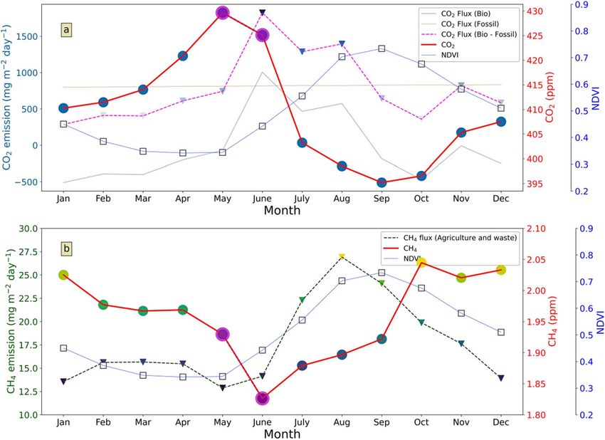
www.nature.com/scientificreports/
Figure 2. Seasonal variation of (a) CO2 and (c) CH4 at Sinhagad, for the year 2014–2015. The shaded region
shows the standard deviation. Seasonal variations of other sites are also shown in the figure. N.B-Seasonal
variation of knp is obtained in the year 2016, but it is shown in 2015 in the graph for comparison purpose only.
Similarly, cri seasonality33 is obtained from monthly mean data of 2010–2012 but shown in 2015 in the graph
for comparison only. Highlighted markers in sng time series in May and June, 2015 is obtained from weekly flask
samples to fill the gap. Seasonal amplitude (maximum − minimum) of several sites is shown in (b) for CO2 and in
(d) for CH4.
high positive (positive sign denotes CO2 added to the atmosphere) during June–July–August, though atmospheric
CO2 concentration is low (Fig. 4a).
CH4 emission from the agriculture and waste (AW) sector of CT consists of enteric fermentation, animal
waste management, wastewater and landfills, and rice agriculture. Emission from the AW sector is high during
monsoon. The co-occurrence of high NDVI and AW sector emission suggest that rice agriculture is a dominant
part of AW sector emission. In comparison, low surface C H4 concentration is observed in monsoon.
Influence of planetary boundary layer (PBL). The planetary boundary layer (PBL) is the lowermost layer of the
troposphere, where temperature and wind speed plays an essential role in its height variation. The boundary
layer can mix the GHG emitted at the ground level up to a certain height and reduce its concentration near the
ground. So, seasonal changes in the boundary layer may affect the ground concentration of GHGs. Monthly
PBLH is computed by averaging the hourly data and compared with C O2 and CH4 concentrations. Monthly
PBLH is observed to be minimum (maximum) during the monsoon (pre-monsoon). Seasonal PBLH during
monsoon, post-monsoon, winter, and pre-monsoon is 754.8, 1136.45, 1213.72, and 1420.08 m, respectively. The
influence of PBLH on C O2 and CH4 is shown in Supplementary Fig. 2a,b, respectively, for the seasonal transi-
tions, i.e., monsoon to post-monsoon (M-PM), post-monsoon to winter (PM-W), and winter to pre-monsoon
(W-PreM). Here ΔPBLH and ΔGHG’s are calculated from the (later season value − previous season value), i.e.,
ΔPBLH for M-PM means ([PBLH during post-monsoon] − [PBLH during monsoon]).
We find two cases:
1. [ΔPBLHM-PM > ΔPBLHPM-W] leads to [ΔCO2 M-PM < ΔCO2 PM-W] and [ΔCH4 M-PM > ΔCH4 PM-W ]
2. [ΔPBLHW-PreM > ΔPBLHPM-W] leads to [ΔCO2 W-PreM > ΔCO2 PM-W] and [ΔCH4 W-PreM < ΔCH4 PM-W ]
Effect of meteorology in different seasons. A biplot analysis is carried out for each season to identify
the interdependency of several meteorological parameters such as wind speed (WIND), wind direction (dir),
Scientific Reports | (2021) 11:2931 | https://doi.org/10.1038/s41598-021-82321-1 4
Vol:.(1234567890)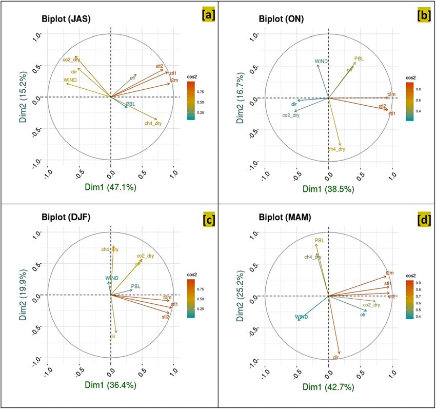
www.nature.com/scientificreports/
Figure 3. (a–d) 10-day back trajectories arriving at Sinhagad at a surface level during monsoon, post-monsoon,
winter, and pre-monsoon.
outgoing longwave radiation (olr), planetary boundary layer (PBL), 2 m-air temperature (t2m), soil temperature
in layer 0–7 cm (stl1) and soil temperature in layer 7–28 cm (stl2) with GHGs (Fig. 5a–d). In the two-dimen-
sional space of two leading principal components, we used the biplot technique29 to describe the PCA result.
The two axes in the biplot represent the first two principal components, and the arrow vectors describe the
variables in this space. Supplementary Fig. 8a–d shows the scree plot for monsoon, post-monsoon, winter, and
pre-monsoon, respectively. Scree plot is the plot of eigenvalues organised from largest to smallest. Here scree
plot is shown in terms of the percentage of explained variance. It is to be noted that in each season, the first two
PCs (PC1 and PC2) are dominant components; hence, biplot analysis is carried out for each season to identify
the interdependency of several meteorological parameters and GHGs. The length of an arrow represents the
variance, and the cosine between two arrows represents the linear correlation between the two variables. All the
variables are scaled to unit variance before performing PCA. The variables that are better explained by the two
principal components will be longer and closer to the unit circle. Acute and obtuse angle represents positive and
negative correlation, respectively, while a right angle implies a lack of correlation.
An anti-correlation between C H4 and wind speed (Fig. 5a) is found in monsoon. The wind rose diagram
(Fig. 1d) also supports this finding. The prevailing south-westerly wind in monsoon is associated with low C H4
values in the wind rose diagram. A positive correlation between CO2 and wind speed is found. This interplay
between CO2 and wind is discussed further in the following section. The association of C O2, CH4 with wind is
reduced in post-monsoon (Fig. 5b). While a positive correlation between CO2 and CH4 is evident in the winter
months (Fig. 5c). The correlation coefficient value between CO2 and CH4 in winter is 0.52 (n = 7108). The close
association of C
H4-PBL and CO2-soil temperature (both layers 1 and 2) is the dominant feature in pre-monsoon
(Fig. 5d).
Influence of prevailing meteorology. Correlation coefficients (R) between wind speed and C O2 (RCO2) during
monsoon, post-monsoon, winter and pre-monsoon are 0.51 (n = 118), 0.15, − 0.02 and − 0.28, while for C H4
are (RCH4) − 0.57 (n = 118), − 0.3, − 0.02 and − 0.27 respectively. A good inverse correlation between GHG and
wind speed suggests that with an increase in wind speeds, GHG concentrations would decrease. In contrast, a
weaker correlation would suggest regional/local transport plays some r ole30,31. Strong wind, especially during
the monsoon season (Supplementary Fig. 1c) is likely to dilute the GHG concentration. This is validated for
Scientific Reports | (2021) 11:2931 | https://doi.org/10.1038/s41598-021-82321-1 5
Vol.:(0123456789)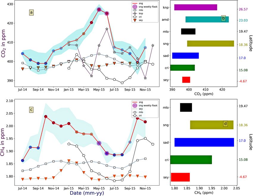
www.nature.com/scientificreports/
Figure 4. (a) Co-variance of CO2 and NDVI calculated over an area of 0.5° × 0.5° for the entire observation
H4, NDVI, and CH4 flux from agriculture and waste of CT-product. N.B-The
period. (b) Co-variation of C
highlighted points in CO2 and CH4 time series denotes data from weekly flask samples.
the case of CH4 in which the wind and CH4 concentration are negatively correlated (RCH4 = − 0.57). But, CO2 is
positively related to wind speed (RCO2 = 0.51). To have further insight into the effect of wind on CO2, we take the
average wind speed integrated over a larger area (up to 11.5° × 4.5°, covering the central to mid-Arabian sea) and
re-calculate the correlation coefficient. The results (summarised below) show that in the case of CO2 the R-value
practically remains the same, but for CH4 it is improved significantly.
a) For area—(18–18.5° N) and (69.5–74° E) gives R
CO2 = 0.53, RCH4 = (− 0.62)
b) For area—(14–18.5° N) and (62.5–74° E) gives R
CO2 = 0.54, RCH4 = (− 0.71)
A strong negative correlation between CH4 and wind presents dilution of CH4 due to intrusion of southern
hemispheric clean air with a strong south-westerly wind of monsoon, schematically shown in Fig. 1a.
Anthropogenic signature on GHG’s probability distribution. To investigate the anthropogenic and
biospheric signature on GHGs, we have partitioned the CO2 and CH4 concentration for the day (07:00–18:00
LT) and night hours (20:00–06:00 LT) for the entire study period. Supplementary Fig. 4a,b shows the prob-
ability distribution (PD) of CH4 and CO2 concentrations during the daytime and nighttime, respectively. Sup-
plementary Fig. 4b shows that the PD of C O2 is narrow (broad) during the night (day) time. Mean daytime and
nighttime CO2 concentrations are 404.6 ± 7.8 ppm (µ ± 1σ) and 407.42 ± 5.93 ppm, respectively. On the other
hand, the C H4 concentration in the daytime and nighttime are practically the same. The respective mean values
are 1.974 ± 0.078 ppm and 1.968 ± 0.07 ppm. We
have also calculated the skewness (S) and kurtosis (K) of these
distributions. The lower skewness SCO2 = 0.04 for nighttime distributions than that of the daytime distribu-
tion SCO2 = 0.16 implies that the nighttime distribution is more symmetric. The same is the case for C H4, for
which the values are 0.37 and 0.97, respectively. This means the nighttime distributions are more constrained.
For CO2, the kurtosis values for both day (0.52) and nighttime (1.20) are much lower than those obtained for a
normally distributed curve, which is 3. This may imply that the extreme values are less relative to the normally
distributed curve, but compared to daytime, the nighttime emissions are characterised by a slightly more num-
ber of extreme values. However, C H4 shows the opposite behaviour, since the kurtosis value for daytime (2.7) is
higher than that of the nighttime (− 0.24).
The probability distribution of CO2 and CH4 of day and nighttime data has also been carried out for different
seasons. Supplementary Figs. 5a–d and 6a–d show the results. As found earlier, the monsoon season daytime PD
Scientific Reports | (2021) 11:2931 | https://doi.org/10.1038/s41598-021-82321-1 6
Vol:.(1234567890)www.nature.com/scientificreports/
Figure 5. Biplot in PC1 and PC2 space showing the association of individual variables and their phase
relationship for (a) monsoon (July–August–September), (b) post-monsoon (October–November), (c) winter
(December–January–February), and (d) pre-monsoon (March–April–May).
Monsoon Post-monsson Winter Pre-monsoon
Day Night Day Night Day Night Day Night
CO2 400.22 ± 5.48 406.57 ± 3.96 401.845 ± 6.27 404.05 ± 5.55 409.877 ± 4.51 409.56 ± 4.06 416.953 ± 5.43 417.01 ± 4.6
CH4 1.903 ± 0.0415 1.904 ± 0.0406 2.028 ± 0.0596 2.0204 ± 0.053 2.002 ± 0.0722 1.987 ± 0.0503 1.963 ± 0.0444 1.967 ± 0.0451
Table 1. Season wise average concentration and standard deviation of GHGs during day and night.
is characterised by a broad peak, but the nighttime PD is relatively narrow. The nighttime mean (Supplemen-
tary Fig. 5a) is right-shifted, as there is practically no sink of C
O2. The post-monsoon season shows a broader
spectrum for both the period (Supplementary Fig. 5b), indicating an increase in the nighttime source of C O 2.
The PDs for the winter (DJF) and the pre-monsoon season (MAM) are quite broad, and they show similar
characteristics (Supplementary Fig. 5c,d). Another feature of these distributions is the range of daytime C O 2:
the monsoon season has a range of 385–410 ppm, and the post-monsoon season 385–415 ppm. At the same
time, the winter season shows a range of 402–425 ppm and the pre-monsoon season 405–435 ppm. Throughout
the monsoon, the mean CO2 concentration is 400.22 ± 5.48 ppm during the day, whereas an elevated CO2 level,
406.57 (~ 6.35 ppm more than daytime) with low SD, is a vital feature of the nighttime variability (Table 1). This
difference is also noticeable through the post-monsoon (ON), but the difference of mean day and night CO2
concentration gets decreased. During the winter and pre-monsoon (DJF and MAM) the difference during the
day and night C O2 concentration almost vanishes.
Scientific Reports | (2021) 11:2931 | https://doi.org/10.1038/s41598-021-82321-1 7
Vol.:(0123456789)www.nature.com/scientificreports/
Figure 6. Diurnal variation of seasonal C
O2, CH4, and planetary boundary layer height (PBL) during (a)
monsoon, (b) post-monsoon, (c) winter, and (d) pre-monsoon.
JAS (monsoon) ON (post-monsoon) DJF (winter) MAM (pre-monsoon)
CO2 (ppm) 10.01 4.133 1.98 2.75
CH4 (ppb) 5.3 28.79 62.05 40.96
Table 2. Amplitude (maximum − minimum) of diurnal variation for the different seasons.
In comparison, C H4 does not show any significant daytime and nighttime variation in most seasons except
winter. Figure 4b and Table 1 reveal a significant seasonal variation of CH4, but day–night variation in intra-
seasonal timescale existed only in winter. Wintertime day and night mean CH4 concentration differs by 15 ppb.
High mean CH4 in daytime indicates the source, and higher SD represents diversity in source processes of
CH4 than night. This is also reflected in the S and K values of methane; the daytime values are high (S = 2.58,
K = 11.33) for the winter season (DJF). Similarly, the pre-monsoon season (MAM) also shows relatively higher
values (S = 2.28, K = 9.90). This means that methane concentrations in this region remain high from November
through March due to enhanced emission and/or reduced loss due to the reduction in the OH r adical32.
Diurnal variation of CO2 and CH4. Figure 6a–d show the diurnal cycle of CO2 and CH4 over the sng site
averaged over a seasonal cycle. During the monsoon season (Fig. 6a), the diurnal pattern of C O2 remains high in
the early morning and then steadily decreases due to increased photosynthetic activity and becomes minimum
around 13:00 LT. In the post-monsoon season (Fig. 6b), the minimum value is shifted to 10:00 LT. For the winter
season and pre-monsoon (Fig. 6c,d), the patterns are very different; the maximum and minimum values are not
well defined, and the diurnal pattern is somewhat linear. A large deviation from the monsoonal-pattern during
the winter and pre-monsoon strongly indicates a weakening biospheric role and increased anthropogenic activi-
ties driving the diurnal behaviour of CO2 concentration in these seasons. On the other hand, the diurnal pattern
of CH4 during the monsoon is not well defined. The patterns, however, are quite different for the other seasons,
as illustrated in Fig. 6b–d; the minimum in the early hours and the maxima around 10:00 LT. The pre-monsoon
season also gets second maxima around 19:00 LT.
Figure 6a–d shows the seasonal variation of the diurnally averaged Planetary Boundary Layer Height (PBLH)
in association with CH4 and CO2, respectively. Table 2 shows the amplitude, i.e., the difference between the diur-
nal minima and the maxima for different seasons. The table indicates that the diurnal variation of CO2 is low
during the winter or pre-monsoon time (1.98 and 2.75 ppm, respectively). The variability is increased during
post-monsoon (4.1 ppm) and obtains maximum amplitude (10.01 ppm) during the monsoon. Moreover, it is
noted that PBL height attains its maximum value around 14:00–15:00 LT for almost every season while the time
of lowest CO2 is different for different seasons. CO2 reaches a minimum of around 10:00 LT during post-monsoon
(Fig. 6a,b), shifted to 12:00–13:00 LT during monsoon. This shifting may be related to the amount of vegetation
Scientific Reports | (2021) 11:2931 | https://doi.org/10.1038/s41598-021-82321-1 8
Vol:.(1234567890)www.nature.com/scientificreports/
around the site. Figure 4a suggests that NDVI (a proxy of vegetation) is high during October–November, which
may lead to enhance photosynthesis during the noon hours (11:00–12:00 LT).
Some interesting features are observed during the period 00:00–06:00 LT. CO2 levels remain somewhat con-
stant for the monsoon and post-monsoon periods. Constant levels at night during monsoon and post-monsoon
give evidence of continuous but weak sources such as plant and soil respiration. C
H4 shows a maximum (mini-
mum) diurnal amplitude (Table 2) of 62.05 (5.3) ppb during winter (monsoon). The monsoon to post-monsoon
transition phase experiences the maximum increase in C H4 amplitude (around 443%). On the other hand, the
pre-monsoon to monsoon transition registers a modest decrease (~ 87%) in CH4 diurnal amplitude.
Discussion and conclusions
The seasonal amplitude of CO2, is high over sng as compared to knp (forest site), amd (urban site) and sad (semi-
urban site) of India. The seasonality of knp-CO2 is mostly driven by the biosphere. Pre-monsoon rainfall in knp
enhances Leaf Area Index (LAI), which in turn increases C O2 assimilation during d aytime11 hence reducing the
atmospheric CO2 concentration. While, during monsoon, though LAI is high, occasional overcast conditions
reduce photosynthetically active radiation (PAR) from reaching the canopy, reducing the C O2 uptake. Simulta-
neously, sad shows enhanced C O2 concentration in pre-monsoon months due to higher temperature and solar
radiation26 and minimum in monsoon mostly driven by enhanced photosynthesis with the availability of higher
soil moisture. C O2 mixing ratio over cri is highest in February–March, due to increased heterotrophic respira-
tion and anthropogenic activity in northern I ndia33. The high seasonal amplitude of sng is characterised by low
CO2 in monsoon and post-monsoon and elevated CO2 during pre-monsoon season. The steady growth of C O2
during the dry season (November to May) indicates a decreasing trend of vegetation uptake in the neighbour-
ing regions (Fig. 4a). A sharp increase in mean value (410–417 ppm) during the pre-monsoon period could be
attributed to enhanced solar radiation. Higher temperature enhances C O2 photosynthesis during daytime and
respiration during the nighttime34. In that case, the diurnal amplitude (maximum–minimum) of CO2 should
be high, but during pre-monsoon, this amplitude becomes negligible (discussed in diurnal variation of GHG
section). Soil respiration and biomass burning also act as a source of C O2 into the atmosphere. With the advance-
ment of monsoon season, the CO2 concentration steadily reduces mainly due to the CO2 uptake by the biosphere.
Additionally, the reduction in temperature further decreases the leaf and soil r espiration35,36. Moreover, NDVI
(a proxy of vegetation) is increasing (Fig. 4a) during monsoon months.
CH4 concentrations over monsoon Asia (including China) show higher values during the wet seasons (JAS
and ON) and low values during dry periods (DJF and MAM) driven by agricultural practices, i.e., paddy fields as
well as large scale transport and c hemistry37,38. Like the ’background’ region, mlo in the Pacific Ocean, we have
also observed low methane concentrations during the summer months (JAS, Fig. 2c) though the mechanism is
not the same as that of mlo. In our case, low concentration is controlled by strong monsoon circulation though
surface emission (from AW sector, Fig. 4b) is high. Low surface C H4 concentration instead of high local emis-
sion is also found by Guha et al.39. They suggest the intrusion of southern hemispheric clean air with monsoonal
south-westerly wind is responsible for low surface C H4 concentration. Therefore, maximum C H4 concentration
is found during post-monsoon when south-westerly current is decreased.
In comparison, the second maximum of C H4 emission is observed in February–March–April with very low
NDVI. Hence, emission from wastewater and landfills, enteric fermentation, and animal waste management plays
a dominant role in C H4 emission during February–March–April. It is found that boundary layer dynamics is not
sufficient for the seasonal change of CO2 and CH4 levels. In a nutshell, the tropospheric CH4 concentration in this
region is determined by the following processes: a balance between the local to regional scale surface emission,
destruction by the OH radicals at the hemispheric scale, and the regional monsoon circulation. Meanwhile, a
low concentration of CO2 instead of high positive residual flux (biosphere + fossil) indicates that monsoon flow
brings cleaner air, which lowers the average concentration of atmospheric C O2 over sng as observed for C H 4.
Hence, we found a strong negative correlation between wind speed and C H4. But interestingly, a positive cor-
relation is evident between CO2 and wind speed in monsoon.
Monsoon rainfall frequently comprises wet and dry spells of precipitation over a period of 10–90 days, widely
known as monsoon intraseasonal oscillation (ISO). 10–20 days40 and 20–60 days41,42 are two dominant modes
of ISO. Cross equatorial low-level jet (LLJ, surface south-westerly wind) is a dominant feature of monsoon. LLJ
also shows intraseasonal oscillation in association with monsoon ISO43 or precisely with north/north-eastward
propagation of deep convection44, but with a lag of about 2–3 days. Valsala et al.45 also show the interplay between
monsoon ISO and net biosphere C O2 flux. OLR is considered a proxy for the deep convection and is used for
precipitation estimation46–48. A lag correlation analysis is carried out between filtered (10–60 days band passed)
wind vs. filtered OLR and filtered CO2 vs. filtered wind (see “Supplementary section”). A maximum correlation
is observed between OLR and wind when OLR leads the wind by 2–3 days.
In contrast, C O2 shows a strong positive correlation with the wind, with wind lagging 1–2 days. Hence, the
positive correlation between CO2 and wind may arise due to the response of monsoon intraseasonal oscillation.
A strong monsoon circulation brings cleaner air, which reduces the CO2 and C H4 both, but C O2 is modulated
by biospheric uptake. The biosphere uptake is further modulated by monsoon intraseasonal oscillation. Conse-
quently, we found a positive relation between CO2 and wind as a response to monsoon.
A higher SD of C O2 histogram during the daytime indicates a broader spread with respect to the nighttime
distribution, which is characterised by a lower SD. So, the broadness of the CO2 distribution function during the
daytime is caused by a diverse source/sink of C O2. With the development of the boundary layer, C O2 gets mixed
vertically. As the day progress, the photosynthetic CO2 sink reduces the CO2 concentration, which is moderated
by the increase in PBLH. While anthropogenic sources of CO2 and plant respiration are also active during the
day, a broader C O2 distribution spectrum is yielded during different hours of the day. The narrow PD for CO2
Scientific Reports | (2021) 11:2931 | https://doi.org/10.1038/s41598-021-82321-1 9
Vol.:(0123456789)www.nature.com/scientificreports/
in the nighttime is suggesting the dominating role of C O2 release by respiration and anthropogenic activity. The
difference between daytime and nighttime CO2 distribution is evident in monsoon and post-monsoon only.
Moreover, the diurnal variation of CO2 is also most prominent in these seasons. Daytime CO2 minima (around
noon), a constant value of C O2 during the night (00:00–06:00 LT), different daytime and nighttime C O2 histo-
gram are the key features in monsoon and post-monsoon season. In contrast, the diurnal variation of C O2 in
winter and pre-monsoon diminishes. Though, daytime PBLH maximum is more (> 2000 and > 2500 m) during
winter and pre-monsoon (Fig. 6c,d), which indicates a strong mixing. This clearly shows that the monsoon and
post-monsoon season get their CO2 share mainly from the active biosphere. In contrast, the other two seasons
get from the degradation of the biosphere and anthropogenic activities. Boundary layer dynamics are ineffective
when vegetation is less. Moreover, the close association of soil temperature at level1 and 2 with C O2 (Fig. 5d)
implies that soil respiration is a dominant part of pre-monsoon C O 2.
A similar pattern in C H4 histogram during daytime and night time implies that the source and transport
processes of CH4 remain more or less invariant (note that the CH4 sink by OH is a slow process, with a time
scale of 1 year or longer in summer over the tropics; Patra et al.17). Diurnal variation of CH4 (Fig. 6a–d) shows
morning CH4 develops with the advent of PBLH other than monsoon. Such a pattern suggests, trapped C H4 in
the neighbouring valley due to a stable boundary layer of the previous night becomes available at our site (top of
a hill) with the rise in the boundary layer in the morning hours. So, we get a morning peak in C
H4 concentration.
As PBLH grows beyond the site elevation, CH4 drops due to mixing with a larger area. Winter is characterised
by a small peak in CH4 levels (Fig. 6c) at the evening (around 19:00 LT), which further develops and emerges
as a dominant peak in pre-monsoon. Hence, a close association of PBL and CH4 is observed in biplot in pre-
monsoon (Fig. 5d).
Data and methodology. Climatology of the study area. The mean monthly variation of relative humid-
ity (RH in %) and temperature (°C) from NCEP-FNL reanalysis dataset over sng is shown in Supplementary
Fig. 1a,b during the period 2014–2015. Temperature over sng varies from ~ 25 to ~ 31 °C. Relative humidity
(RH) was maximum during south-west monsoon (June-July–August–September, JJAS) season of > 75%, and the
minimum occurred during winter (December–January–February, DJF) of about < 50%. At sng, the wind speed at
850 hPa (data source: ERA-Interim) varies between 1 and 12 ms−1. Maximum wind speed occurred mainly from
the south-west direction during the Indian summer monsoon (ISM) months, JJAS, which originated from the
Arabian Sea. In winter, the winds are mostly from the northeast direction, originated from the Indian subcon-
tinent (Supplementary Fig. 1c,d). Figure 1b shows the location of the study area with the mean outgoing long-
wave radiation (shaded) and mean wind (1000 hPa) flow in vector form. Figure 1a depicts the south-westerly
monsoon flow from the ocean to land with enhancing convection (low OLR) over the Indian sub-continent. Fig-
ure 1b illustrates an opposite flow pattern during the winter associated with suppressing convection (high OLR).
So, it is evident that our study area experiences a strong seasonally reversing of the wind flow from summer to
winter. The wind rose diagram shows south-westerly wind is associated with low CO2 and CH4 concentration
(Fig. 1c,d). The interplay between wind and GHG concentration is discussed further in “Influence of prevailing
meteorology” section.
GHG analyser. Continuous air sampling was done through a fast greenhouse gas analyser (model: LGR-
FGGA-24r-EP) from a 10 m meteorological tower. It is based on enhanced off-axis integrated cavity output spec-
troscopy (OA-ICOS) technology49. This instrument is able to provide C H4, CO2, and H
2O concentration simul-
taneously with high temporal resolution (up to 1 Hz). The sensor was calibrated using a zero air cylinder having
known CO2, CH4 concentrations. The ’dry values’ of CO2 and CH4 mixing ratios, corrected for water vapour, are
reported in this paper. The C
O2 and CH4 data integrated for 100-s intervals are presented here. The analyser has
0.3 ppb, 0.05 ppm, and 5 ppm precision of CH4, CO2, and H2O when operating in the 0.01 Hz frequency. Moreo-
ver, we take 15-min average C O2 and C H4 measurements for further analysis. The site has been operational
from July-2014 to November-2015. There were several data gaps in between, with an opening from 3-May-2015
to 9-July 2015 (longest gap), due to instrument maintenance. This gap is filled with weekly flask samples data24
obtained from the same site. CO2 and CH4 concentration data have been plotted on diurnal and monthly time
scales. The year was divided into four different seasons, i.e., monsoon (July–August–September), post-monsoon
(October–November), winter (December–January–February), and pre-monsoon (March–April–May).
Due to the unavailability of AWS in the study area, no in-situ meteorological data were available; instead, we
use different kinds of reanalysis data as mentioned later.
Kaziranga (knp) CO2 data. The Metflux India flux observational site Kaziranga National Park (knp) is
a semi-evergreen forest located in the north-eastern state of Assam. The CO2 concentration over the forest is
measured at the height of 37 m using an enclosed path CO2–H2O infrared gas analyser (LI-7200, LI-COR, USA)
at frequency of 10 Hz. The high-frequency data are processed using the EddyPro software and averaged in the
time interval of 15 min. The details of the study area and instruments can be found i n11.
Moderate‑resolution imaging spectrometer (MODIS). The MODIS was launched in December 1999
on the polar-orbiting NASA-EOS Terra platform50,51. It has 36 spectral channels covering visible, near-infrared,
shortwave infrared, and thermal infrared bands. In the present study, we have used 5-km spatial resolution hav-
ing 16-day temporal resolution NDVI (Normalized difference vegetation index) data. We got the dataset from
MODIS (Product-MOD13C1) official website ("https://modis.gsfc.nasa.gov/data/dataprod/mod13.php"). The
NDVI is a normalised transform of the near-infrared (NIR) to red reflectance ratio (RED) and calculated using
the following equation
Scientific Reports | (2021) 11:2931 | https://doi.org/10.1038/s41598-021-82321-1 10
Vol:.(1234567890)www.nature.com/scientificreports/
NIR − RED
NDVI =
NIR + RED
NDVI values range from − 1.0 to + 1.0. Higher positive values are associated with increased vegetation coverage.
The NDVI is averaged over the region 18–18.5° N and 73.5–74° E.
Outgoing longwave radiation. Outgoing longwave radiation (OLR) is the radiative flux leaving the
earth-atmosphere in the infrared region. OLR has a broad wavelength ranging from 4 to 100 µm. In the present
study, we have been using OLR data from a very high-resolution radiometer (VHRR), onboard Kalpana-1 satel-
lite. VHRR measures OLR in infrared (10.5–12.5 µm) and water vapour (5.7–7.1 µm) wavelength band. Retrieval
algorithm of OLR from the VHRR images, archived at the National Satellite Data Centre of the India Meteoro-
logical Department, New Delhi, is available in52. The OLR data is available at three-hour intervals (i.e. 00, 03, …,
18 and 21 UTC) starting from May-2004 over the Indian region (40° S–40° N, 25° E–125° E). It has 0.25° × 0.25°
spatial resolution. In the present study, we used daily data. The yearly data files are available on the official site
of IITM, Pune ("https://www.tropmet.res.in/~mahakur/Public_Data/index.php?dir=K1OLR/DlyAvg"). Usually,
low OLR values (< 200 W m−2) denote convection, whereas high values indicate clear sky. OLR is averaged over
the region 18.12–18.62° N and 73.62–74.12° E.
Modern‑era retrospective analysis for research and applications (MERRA). The MERRA-2 is a
NASA atmospheric reanalysis project that began in 1980. It replaced the original MERRA53 reanalysis product
using an upgraded version of the Goddard Earth Observing System Model, Version 5 (GEOS-5) data assimi-
lation system. MERRA-2 includes updates to the m odel54 and Global Statistical Interpolation (GSI) analysis
scheme of Wu et al.55. MERRA-2 has a spatial resolution of 0.625° × 0.5°. In the present study, we used MERRA-2
dataset to determine the Planetary Boundary Layer Height on an hourly timescale. We take planetary boundary
later height (PBLH) averaged over 18–18.5° N and 73.13–74.38° E for our study region.
European re‑analysis‑interim (ERA‑Interim). Era-Interim is a reanalysis product of the global atmos-
phere produced by the European Centre for Medium-Range Weather Forecast (ECMWF) available from 197956.
The Era-Interim atmospheric model and reanalysis system uses cycle 31r2 of ECMWF’s Integrated Forecast
System (IFS). The system includes 4-dimensional variational analysis (4D-Var) with a 12-h analysis window. In
each window, available observations are combined with prior information from a forecast model to estimate the
evolving state of the global atmosphere and its underlying surface. Meridional and zonal wind components at
850 hPa at a spatial resolution of 0.25° × 0.25° (grid dimension: 18–18.5° N and 73.5–74° E) were used.
ERA5. ERA5 is the latest version of reanalysis produced by ECMWF. ERA5 is produced using 4D-Var data
assimilation in ECMWF’s Integrated Forecast System. A temporal resolution of 1 h and a vertical resolution of
137 hybrid sigma model levels. The 37 pressure levels of ERA5 are identical to ERA-Interim57. ERA5 assimilates
improved input data that better reflects observed changes in climate forcing and many new or reprocessed obser-
vations that were not available during the production of ERA-Interim.
ERA5-Land provides the land component of the model without coupling to the atmospheric models. It
uses the Tiled ECMWF Scheme for Surface Exchanges over Land with revised land-surface hydrology (HTES-
SEL, CY45R1). It is delivered at the same temporal resolution as ERA5 and with a higher spatial resolution of
0.1° × 0.1°. 2 m air temperature, soil temperature level 1 (0–7 cm), and soil temperature at level 2 (7–28 cm) is
used.
NCEP FNL re‑analysis. The NCEP FNL (final) operational global analysis data are on 1° × 1° grid prepared
operationally every six hour. This product comes from the Global Data Assimilation System, which continually
gathers observational data. The time series of the archive is continually extended to a near-current date but not
preserved in real-time (http://rda.ucar.edu/datasets/ds083.2/). The key aim of these re-analysis data is to provide
compatible, high-resolution, and high-quality historical global atmospheric datasets for use in weather research
communities58, 59. Air temperature and RH are averaged over the area 18–19° N and 73–74° E.
Received: 10 October 2020; Accepted: 19 January 2021
References
1. Ciais, P. et al. Carbon and other biogeochemical cycles. in Climate Change 2013: The Physical Science Basis. Contribution of Working
Group I to the Fifth Assessment Report of the Intergovernmental Panel on Climate Change Change (2013).
2. Stocker, T. F. et al. Contribution of working group I to the fifth assessment report of the intergovernmental panel on climate change.
Clim. Change 2013 Phys. Sci. Basis. https://doi.org/10.1017/CBO9781107415324 (2013).
3. Tans, P. P., Berry, J. A. & Keeling, R. F. Oceanic 13C/12C observations: A new window on ocean CO2 uptake. Glob. Biogeochem.
Cycles 7, 353–368 (1993).
4. Keeling, C. D., Whorf, T. P., Wahlen, M. & van der Plichtt, J. Interannual extremes in the rate of rise of atmospheric carbon dioxide
since 1980. Nature 375, 666–670 (1995).
5. Quéré, C. L. et al. Global carbon budget 2017. Earth Syst. Sci. Data 10, 405–448 (2018).
6. Patra, P. K., Maksyutov, S. & Nakazawa, T. Analysis of atmospheric C O2 growth rates at Mauna Loa using C O2 fluxes derived from
an inverse model. Tellus B Chem. Phys. Meteorol. 57, 357–365 (2005).
Scientific Reports | (2021) 11:2931 | https://doi.org/10.1038/s41598-021-82321-1 11
Vol.:(0123456789)www.nature.com/scientificreports/
7. Schimel, D. S. et al. Recent patterns and mechanisms of carbon exchange by terrestrial ecosystems. Nature 414, 169–172 (2001).
8. Zobitz, J. M., Keener, J. P., Schnyder, H. & Bowling, D. R. Sensitivity analysis and quantification of uncertainty for isotopic mixing
relationships in carbon cycle research. Agric. For. Meteorol. 136, 56–75 (2006).
9. Ciais, P. et al. Partitioning of ocean and land uptake of CO 2 as inferred by δ13C measurements from the NOAA climate monitoring
and diagnostics laboratory global air sampling network. J. Geophys. Res. 100, 5051 (1995).
10. Chatterjee, A. et al. Biosphere atmosphere exchange of CO2, H2O vapour and energy during spring over a high altitude Himalayan
forest at Eastern India. Aerosol Air Qual. Res. https://doi.org/10.4209/aaqr.2017.12.0605 (2018).
11. Sarma, D. et al. Carbon dioxide, water vapour and energy fluxes over a semi-evergreen forest in Assam, Northeast India. J. Earth
Syst. Sci. 127, 94. https://doi.org/10.1007/s12040-018-0993-5 (2018).
12. Etheridge, D. M., Steele, L. P., Francey, R. J. & Langenfelds, R. L. Atmospheric methane between 1000 A.D. and present: Evidence
of anthropogenic emissions and climatic variability. J. Geophys. Res. Atmos. 103, 15979–15993 (1998).
13. Dlugokencky, E. J., Nisbet, E. G., Fisher, R. & Lowry, D. Global atmospheric methane: Budget, changes and dangers. Philos. Trans.
R. Soc. Lond. A Math. Phys. Eng. Sci. 369, 2058–2072 (2011).
14. Keppler, F., Hamilton, J. T. G., Braß, M. & Röckmann, T. Methane emissions from terrestrial plants under aerobic conditions.
Nature 439, 187–191 (2006).
15. Garg, A., Kankal, B. & Shukla, P. R. Methane emissions in India: Sub-regional and sectoral trends. Atmos. Environ. 45, 4922–4929
(2011).
16. Patra, P. K. et al. TransCom model simulations of CH4 and related species: Linking transport, surface flux and chemical loss with
CH4 variability in the troposphere and lower stratosphere. Atmos. Chem. Phys. 11, 12813–12837 (2011).
17. Patra, P. K. et al. Growth rate, seasonal, synoptic, diurnal variations and budget of methane in the lower atmosphere. J. Meteorol.
Soc. Jpn. Ser. II 87, 635–663 (2009).
18. Lin, X. et al. Long-lived atmospheric trace gases measurements in flask samples from three stations in India. Atmos. Chem. Phys.
15, 9819–9849 (2015).
19. Ganesan, A. L. et al. The variability of methane, nitrous oxide and sulfur hexafluoride in Northeast India. Atmos. Chem. Phys. 13,
10633–10644 (2013).
20. Schuck, T. J. et al. Greenhouse gas relationships in the Indian summer monsoon plume measured by the CARIBIC passenger
aircraft. Atmos. Chem. Phys. 10, 3965–3984 (2010).
21. Clark-Thorne, S. T. & Yapp, C. J. Stable carbon isotope constraints on mixing and mass balance of CO2 in an urban atmosphere:
Dallas metropolitan area, Texas, USA. Appl. Geochem. 18, 75–95 (2003).
22. Chandra, N., Lal, S., Venkataramani, S., Patra, P. K. & Sheel, V. Temporal variations of atmospheric CO2 and CO at Ahmedabad
in western India. Atmos. Chem. Phys. 16, 6153–6173 (2016).
23. Ballav, S., Naja, M., Patra, P. K., Machida, T. & Mukai, H. Assessment of spatio-temporal distribution of CO2 over greater Asia
using the WRF-CO2 model. J. Earth Syst. Sci. 129, 80 (2020).
24. Tiwari, Y. K., Vellore, R. K., Kumar, K. R., van der Schoot, M. & Cho, C.-H. Influence of monsoons on atmospheric CO2 spatial
variability and ground-based monitoring over India. Sci. Total Environ. 490, 570–578 (2014).
25. Debburman, P., Sarma, D., Williams, M., Karipot, A. & Chakraborty, S. Estimating gross primary productivity of a tropical forest
ecosystem over north-east India using LAI and meteorological variables. J. Earth Syst. Sci. 126, 1–16 (2017).
26. Sreenivas, G. et al. Influence of meteorology and interrelationship with greenhouse gases (CO2 and CH4) at a suburban site of
India. Atmos. Chem. Phys. 16, 3953–3967 (2016).
27. Nath, B. Quantitative assessment of forest cover change of a part of Bandarban Hill tracts using NDVI techniques. J. Geosci. Geomat.
2, 21–27 (2014).
28. Aburas, M. M., Abdullah, S. H., Ramli, M. F. & Ash’aari, Z. H. Measuring land cover change in Seremban, Malaysia using NDVI
index. Proc. Environ. Sci. 30, 238–243 (2015).
29. Gabriel, K. R. The biplot graphic display of matrices with application to principal component analysis. Biometrika 58, 453–467
(1971).
30. Ramachandran, S. & Rajesh, T. A. Black carbon aerosol mass concentrations over Ahmedabad, an urban location in western India:
Comparison with urban sites in Asia, Europe, Canada, and the United States. J. Geophys. Res. Atmos. 112, D06211. https://doi.
org/10.1029/2006JD007488 (2007).
31. Mahesh, P. et al. Impact of land-sea breeze and rainfall on C O2 variations at a coastal station. J. Earth Sci. Clim. Change 5, 1 (2014).
32. Tiwari, Y. K. et al. Understanding atmospheric methane sub-seasonal variability over India. Atmos. Environ. 223, 117206 (2020).
33. Bhattacharya, S. K. et al. Trace gases and C O2 isotope records from Cabo de Rama, India. Curr. Sci. 97, 1336–1344 (2009).
34. Fang, S. X. et al. In situ measurement of atmospheric CO2 at the four WMO/GAW stations in China. Atmos. Chem. Phys. 14,
2541–2554 (2014).
35. Jing, X. et al. The effects of clouds and aerosols on net ecosystem C O2 exchange over semi-arid Loess Plateau of Northwest China.
Atmos. Chem. Phys. 10, 8205–8218 (2010).
36. Patil, M. N., Dharmaraj, T., Waghmare, R. T., Prabha, T. V. & Kulkarni, J. R. Measurements of carbon dioxide and heat fluxes during
monsoon-2011 season over rural site of India by eddy covariance technique. J. Earth Syst. Sci. 123, 177–185 (2014).
37. Hayashida, S. et al. Methane concentrations over Monsoon Asia as observed by SCIAMACHY: Signals of methane emission from
rice cultivation. Remote Sens. Environ. 139, 246–256 (2013).
38. Chandra, N., Hayashida, S., Saeki, T. & Patra, P. K. What controls the seasonal cycle of columnar methane observed by GOSAT
over different regions in India?. Atmos. Chem. Phys. 17, 12633–12643 (2017).
39. Guha, T. et al. What controls the atmospheric methane seasonal variability over India?. Atmos. Environ. 175, 83–91 (2018).
40. Krishnamurti, T. N. & Ardanuy, P. The 10 to 20-day westward propagating mode and “Breaks in the Monsoons”. Tellus 32, 15–26
(1980).
41. Krishnamurti, T. N. & Subrahmanyam, D. The 30–50 days mode at 850 mb during MONEX. J. Atmos. Sci. 39, 2088–2095 (1982).
42. Murakami, T., Nakazawa, T. & He, J. On the 40–50 day oscillations during the 1979 Northern Hemisphere Summer. J. Meteorol.
Soc. Jpn. Ser. II 62, 469–484 (1984).
43. Joseph, P. V. & Sijikumar, S. Intraseasonal Variability of the Low-Level Jet Stream of the Asian Summer Monsoon. J. Climate 17,
1449–1458 (2004).
44. Sikka, D. R. & Gadgil, S. On the maximum cloud zone and the ITCZ over Indian Longitudes during the southwest monsoon. Mon.
Weather Rev. 108, 1840–1853 (1980).
45. Valsala, V. et al. Intraseasonal variability of terrestrial biospheric CO2 fluxes over India during summer monsoons. J. Geophys. Res.
Biogeosci. 118, 752–769 (2013).
46. Liebmann, B. & Gruber, A. Annual variation of the diurnal cycle of outgoing longwave radiation. Mon. Weather Rev. 116, 1659–1670
(1988).
47. Xie, P. & Arkin, P. A. Global monthly precipitation estimates from satellite-observed outgoing longwave radiation. J. Clim. 11,
137–164 (1998).
48. Kemball-Cook, S. R. & Weare, B. C. The onset of convection in the Madden–Julian oscillation. J. Clim. 14, 780–793 (2001).
49. Paul, J. B., Lapson, L. & Anderson, J. G. Ultrasensitive absorption spectroscopy with a high-finesse optical cavity and off-axis
alignment. Appl. Opt., AO 40, 4904–4910 (2001).
Scientific Reports | (2021) 11:2931 | https://doi.org/10.1038/s41598-021-82321-1 12
Vol:.(1234567890)You can also read