Early Science from POSSUM: Shocks, turbulence, and a massive new reservoir of ionised gas in the Fornax cluster
←
→
Page content transcription
If your browser does not render page correctly, please read the page content below
Publications of the Astronomical Society of Australia (PASA)
                                              doi: 10.1017/pas.2021.xxx.

                                              Early Science from POSSUM: Shocks, turbulence, and a massive
                                              new reservoir of ionised gas in the Fornax cluster
arXiv:2102.01702v1 [astro-ph.GA] 2 Feb 2021

                                              C. S. Anderson1,2,3 , G. H. Heald2 , J. A. Eilek1,4 , E. Lenc3 , B. M. Gaensler5 , Lawrence Rudnick6 , C. L. Van
                                              Eck5 , S. P. O’Sullivan7 , J. M. Stil8 , A. Chippendale3 , C. J. Riseley9,10 , E. Carretti10 , J. West5 , J. Farnes11 , L.
                                              Harvey-Smith12,13 , N. M. McClure-Griffiths14 , Douglas C. J. Bock3 , J. D. Bunton3 , B. Koribalski3,13 , C. D.
                                              Tremblay2 , M. A. Voronkov3 , K. Warhurst2
                                              1 Jansky fellow of the National Radio Astronomy Observatory, 1003 Lopezville Rd, Socorro, NM 87801 USA
                                              2 CSIRO   Astronomy and Space Science, PO Box 1130, Bentley WA 6102, Australia
                                              3 ATNF, CSIRO Astronomy and Space Science, PO Box 76, Epping, New South Wales 1710, Australia
                                              4 Physics Department, New Mexico Tech, Socorro NM 87801 USA
                                              5 Dunlap Institute for Astronomy and Astrophysics, University of Toronto, 50 St. George Street, Toronto, ON M5S 3H4, Canada
                                              6 Minnesota Institute for Astrophysics, University of Minnesota, 116 Church St. SE, Minneapolis, MN 55455 USA
                                              7 School of Physical Sciences and center for Astrophysics & Relativity, Dublin City University, Glasnevin, D09 W6Y4, Ireland
                                              8 Department of Physics & Astronomy, The University of Calgary, 2500 University Drive NW, Calgary AB, T2N 1N4, Canada
                                              9 Dipartimento di Fisica e Astronomia, Università degli Studi di Bologna, via P. Gobetti 93/2, 40129 Bologna, Italy
                                              10 INAF - Istituto di Radioastronomia, Via Gobetti 101, 40129 Bologna, Italy
                                              11 Oxford e-Research center (OeRC), Department of Engineering Science, University of Oxford, Oxford, OX1 3QG, UK
                                              12 School of Physics, University of New South Wales, Sydney, NSW 2052, Australia
                                              13 Western Sydney University, Locked Bag 1797, Penrith, NSW, 2751, Australia
                                              14 Research School of Astronomy & Astrophysics, Australian National University, Canberra ACT 2611 Australia

                                              Abstract
                                              We present the first Faraday rotation measure (RM) grid study of an individual low-mass cluster — the Fornax
                                              cluster — which is presently undergoing a series of mergers. Exploiting commissioning data for the POlarisation
                                              Sky Survey of the Universe’s Magnetism (POSSUM) covering a ∼ 34 square degree sky area using the Australian
                                              Square Kilometre Array Pathfinder (ASKAP), we achieve an RM grid density of ∼ 25 RMs per square degree from a
                                              280 MHz band centred at 887 MHz, which is similar to expectations for forthcoming GHz-frequency ∼ 3π-steradian
                                              sky surveys. These data allow us to probe the extended magnetoionic structure of the cluster and its surroundings
                                              in unprecedented detail. We find that the scatter in the Faraday RM of confirmed background sources is increased
                                              by 16.8 ± 2.4 rad m−2 within 1 degree (360 kpc) projected distance to the cluster centre, which is 2–4 times larger
                                              than the spatial extent of the presently-detectable X-ray-emitting intracluster medium (ICM). The mass of the
                                              Faraday-active plasma is larger than that of the X-ray-emitting ICM, and exists in a density regime that broadly
                                              matches expectations for moderately-dense components of the Warm-Hot Intergalactic Medium. We argue that
                                              forthcoming RM grids from both targeted and survey observations may be a singular probe of cosmic plasma in this
                                              regime. The morphology of the global Faraday depth enhancement is not uniform and isotropic, but rather exhibits
                                              the classic morphology of an astrophysical bow shock on the southwest side of the main Fornax cluster, and an
                                              extended, swept-back wake on the northeastern side. Our favoured explanation for these phenomena is an ongoing
                                              merger between the main cluster and a sub-cluster to the southwest. The shock’s Mach angle and stand-off distance
                                              lead to a self-consistent transonic merger speed with Mach 1.06. The region hosting the Faraday depth enhancement
                                              also appears to show a decrement in both total and polarised radio emission compared to the broader field. We
                                              evaluate cosmic variance and free-free absorption by a pervasive cold dense gas surrounding NGC 1399 as possible
                                              causes, but find both explanations unsatisfactory, warranting further observations. Generally, our study illustrates the
                                              scientific returns that can be expected from all-sky grids of discrete sources generated by forthcoming all-sky radio
                                              surveys.

                                              Keywords: galaxies: clusters: individual(Fornax) – galaxies: clusters: intracluster medium – magnetic fields – techniques:
                                              polarimetric – radio continuum: galaxies

                                                                                                                        1
2                                                                                                                   C. S. Anderson et al.

1 INTRODUCTION                                                     as

The Universe’s baryons are mostly located outside the stel-                            P = Q + iU = pIe2iψ                            (1)
lar envelopes of galaxies, in the vast expanses occupied by
clusters of galaxies, and in filaments of tenuous plasma that      After being emitted at a location L, linearly polarised radia-
connect them. The properties of gas in these different regimes     tion will be Faraday rotated by magnetised thermal plasma
— including their state of magnetisation — lie at the heart of     along the line of sight (LOS) to an observer by an amount
theories of cosmic evolution and ecology, but remain difficult     equal to
to pin down observationally. For instance, the hot intraclus-
ter medium (ICM) contains about 4% of the baryonic mass                                    ∆ψ = φ(L)λ2                                (2)
of the late-time Universe, which is (for example) a higher
                                                                   where λ is the observing wavelength, and φ is the Faraday
proportion than is contained in stars (de Graaff et al., 2019).
                                                                   depth, given by
Magnetic fields break the isotropy of viscosity, pressure sup-
port, and thermal conductivity of the ICM, thereby exerting                                    Z       0
an out-sized influence on cluster physics and evolution. They                   φ(L) = 0.812               ne B · ds rad m−2          (3)
can trace ordered and turbulent flows in plasma (e.g. Ander-                                       L

son et al., 2018), reveal interactions between the ICM and         and, in turn, ne [cm−3 ] & B [µG] are the thermal electron
in-falling gas (e.g. Keshet et al., 2017), embedded galaxies       density and magnetic field along the LOS respectively.
(e.g. Dursi & Pfrommer, 2008; Pfrommer & Dursi, 2010) and            The observable polarisation spectrum P (λ2 ) is obtained by
galactic outflows (e.g. Guidetti et al., 2011, 2012; Anderson      summing the polarised emission emerging from all possible
et al., 2018), and help reveal how the broader cosmos became       Faraday depths within the synthesised beam of the telescope:
magnetised (e.g. Vazza et al., 2014; Bonafede et al., 2015).                                 Z ∞
                                                                                                           2
   Beyond the ICM, the Warm-Hot Intergalactic Medium                                P (λ ) =
                                                                                        2
                                                                                                 F (φ)e2iφλ dφ               (4)
(WHIM) must contain around 80% of the Universe’s baryons                                       −∞
(de Graaff et al., 2019), though this material is comparatively       The function F (φ) (the so-called Faraday Dispersion Spec-
unstudied, with only recent claims of detection of its sparser     trum, henceforth FDS) specifies the distribution of polarised
phases (Nicastro et al., 2017; de Graaff et al., 2019; Tanimura    emission as a function of Faraday depth along the LOS. This
et al., 2019; Macquart et al., 2020). Simulations suggest that     quasi-Fourier relationship can be inverted to reconstruct F (φ)
the WHIM will be found in a diverse set of regimes, occupy-        given observations of P (λ2 ) (Burn, 1966; Brentjens & de
ing relatively dense agglomerations (δ ∼ 200, where δ is the       Bruyn, 2005). In the common situation where a point-like
over-density factor of baryons compared to the cosmic mean,        source is viewed through an extended reservoir of magnetised
defined by δ ≡ ρ/ρ̄ − 1, and in turn, ρ is the baryon number       thermal plasma lying in the foreground (which we deal with
density at a given location, while ρ̄ is the mean baryon num-      in this work), F (φ) shows a single peak at a well-defined
ber density in the Universe, which is currently ρ̄ ≈ 2 × 10⁻⁷      Faraday depth φpeak = argmax(|F (φ)|). This is then equiva-
cm−3 ; Planck Collaboration et al., 2016) around galaxy clus-      lent to the so-called Faraday rotation measure (RM) of the
ters in its densest and hottest manifestations, and in tenuous     source. Largely for historic reasons, we continue to use the
filaments between massive galaxies in its sparsest and coolest     term “RM” in places in this work, though the measurements
regimes (δ ∼ a few) (Davé et al., 2001). The magnetisation         themselves are of φpeak — i.e. extracted through the method
of this material is also consequential, since the predictions of   of RM synthesis, rather than from the gradient of the polari-
models for cosmic magneto-genesis differ most strongly here        sation angle as a function of λ2 . Regardless of nomenclature,
(e.g. Donnert et al., 2018 and references therein), which is       φpeak provides a direct measure of the amount of magnetised
just now beginning to be revealed with extraordinary new low       thermal plasma that has been traversed along the line of sight.
frequency radio measurements (Govoni et al., 2019; Botteon         Ensembles of polarised radio sources can therefore back-
et al., 2020), and may also be probed via measurements of          illuminate the magnetoionic structure of extended plasma
radio polarisation and Faraday rotation (e.g. Akahori et al.,      reservoirs in the foreground.
2018; Locatelli et al., 2018; O’Sullivan et al., 2020).               Applying these ‘RM grid’ techniques to study the ICM or
   Faraday rotation is an effective tracer of the distribution     WHIM in individual galaxy clusters has historically been diffi-
and properties of rarefied, magnetised cosmic plasma, such as      cult, because past generations of radio instrumentation could
the ICM and WHIM (e.g. Cooper & Price, 1962; Burn, 1966;           only recover a relatively low density of polarised sources
Conway et al., 1974; Kronberg & Simard-Normandin, 1976;            over the required multi-square-degree sky areas (O(1) lin-
Taylor & Perley, 1993; Farnsworth et al., 2011; O’Sullivan         early polarised source per square degree — e.g. Taylor et al.,
et al., 2013; Johnston-Hollitt et al., 2015; Gaensler et al.,      2009), combined with the uncertainty of whether any given
2015; Anderson, 2016). Consider that the linear polarisation       RM grid source is located behind a target cluster, inside it,
state of radio emission can be described by a complex vector       or in the foreground. Fortunately, these limitations will soon
P , related to the Stokes parameters Q and U, the polarisation     be transcended using data from a new generation of radio
angle ψ, the fractional polarisation p and the total intensity I   interferometers and optical redshift surveys. In the former
Fornax cluster magnetic fields 3
domain, the Australian Square Kilometre Array Pathfinder central ∼ 30 kpc of the cluster (Su et al., 2017), and may have
(ASKAP) can routinely measure polarised source densities generated shocks and turbulence on scales up to more than a
of ∼ 25 per square degree over tens of square degrees in degree (Sheardown et al., 2018).
just a few hours (this work, West et al. in prep.), and will Thus, the Fornax cluster differs greatly in its properties
soon survey the entire southern sky at this or greater depth from other relatively nearby massive clusters, including Virgo
for the Polarisation Sky Survey of the Universe’s Magnetism and Coma, and from the massive clusters from which our
(POSSUM; Gaensler et al., 2010). At the same time, deep canonical understanding of the magnetised ICM were chiefly
pointed observations like the MeerKAT (Jonas, 2009) Fornax derived. While our understanding of the magneto-thermal
Survey (Serra et al., 2016) may soon recover ∼hundreds of plasma structures of even large clusters remain incomplete
polarised sources per square degree. Both approaches will (e.g. Johnston-Hollitt et al., 2015; Heald et al., 2020), our ig-
open up the field of observational galaxy cluster astrophysics norance is much more pronounced at the important low-mass
to routine RM grid studies (Heald et al., 2020). end of the halo distribution. Sensitive new RM grid exper-
This paper heralds the dawn of this era by exploiting iments can directly reveal the magnetised gas in such envi-
ASKAP’s unique imaging capabilities to study the ionised ronments, providing sorely needed new data in this sphere.
gas in the Fornax cluster. The Fornax cluster is nearby (20.64 In this work then, our overarching aim is to search for Fara-
megaparsecs; Mpc; Lavaux & Hudson, 2011), but much day RM enhancements to trace the structure of magnetised
poorer than similarly well-studied clusters like the Virgo and ionised gas in an individual low-mass galaxy cluster for the
Coma clusters. It has only ∼ 390 member galaxies (which are first time. Our specific goals are to (a) estimate the mass and
typically low in mass; Maddox et al., 2019), and has a com- extent of any such material, and to compare these estimates
paratively low total mass of 6+3 13
−1 × 10 M (Drinkwater et al.,
to those determined for ensembles of the more massive clus-
2001; Nasonova et al., 2011; Maddox et al., 2019), which is ters previously probed in RM stacking experiments, (b) to
one and two orders-of-magnitude less massive than the Virgo determine whether any material thereby revealed differs in
and Coma clusters respectively. The (presently detectable) its properties or extent from that revealed by Bremsstrahlung
X-ray-emitting ICM is also small, extending asymmetrically radiation, thus establishing the complementarity of the two
outward from NGC1399 to a mere 15%–30% of the clus- measurement techniques, and (c) demonstrate what unique
ter’s 1.96 degree virial radius. Nevertheless, its halo mass is information the RM measurements provide about the dynami-
more representative of that in which the majority of the galax- cal mass assembly processes that continue to take place in the
ies in the Universe reside and evolve (Haan & Braun, 2014 system. The spatial density and areal sky coverage of our RM
and references therein). The dynamical state of the cluster, grid, coupled the fact that it is dominated by confirmed back-
and associated astrophysical processes, are therefore of keen ground radio sources (as we will show), is groundbreaking in
interest. this field.
Our understanding of the dynamics of this system is evolv- Our paper is organised as follows. We describe our obser-
ing rapidly. The core of the Fornax cluster is densely popu- vations, calibration, and imaging procedures in Section 2, and
lated with early-type galaxies that possess relatively uniform our polarimetric analysis in Section 3. Analysis of ancillary
properties and low velocity dispersion. This used to be cited redshift data is presented in Section 4. We present our results,
as evidence that the Fornax cluster is virialised and well- discussion, and conclusions in Sections 5, 6 and 7 (respec-
evolved (see Iodice et al., 2019 and references therein), but tively). In this paper, we adopt a distance to NGC 1399 of
it is now clear that the Fornax cluster possesses complex D = 20.64 Mpc (Lavaux & Hudson, 2011), which yields an
spatial sub-structure both in terms of its constituent gas and image scale of 100 parsecs/arcsec. Cardinal directions are
galaxies (e.g. Drinkwater et al., 2001; Paolillo et al., 2002; referred to by their usual abbreviations — e.g. NE, SW, S
Scharf et al., 2005; Su et al., 2017; Venhola et al., 2018; for northeast, southwest, and south, respectively. We use the
Sheardown et al., 2018), and is still assembling mass through spectral index convention S ∝ να .
a series of on-going mergers. At the largest scales, Drinkwa-
ter et al. (2001) argue that there is a genuine mass partition
2 OBSERVATIONS, CALIBRATION AND
between northeast and southwest sub-components of the clus-
IMAGING
ter, which are respectively dominated by the cD-type galaxy
NGC 1399 and NGC 1316 — the host galaxy of the radio We observed the Fornax cluster region during commissioning
source Fornax A — a few degrees (∼ 1.3 Mpc) away. Scharf tests of the ASKAP radio telescope (DeBoer et al., 2009;
et al. (2005) cite the swept-back (to the northeast) morphol- Johnston et al., 2007; Schinckel & Bock, 2016). ASKAP
ogy of the hot ICM traced by X-rays as possible evidence consists of 36 × 12-m antennas, each equipped with a Phased
that these sub-components are merging at transonic speeds. Array Feed (PAF), yielding a ∼ 30 square degree instanta-
On smaller scales, NGC 1399 is undergoing a series of close neous field of view (depending on frequency) and high survey
encounters with the spiral galaxy NGC 1404, as the latter speed. We observed a single such pointing for six hours with
falls into the cluster potential and interacts with the diffuse a square_6x6 beam footprint (McConnell et al., 2016), us-
gas there (Machacek et al., 2005). This appears to have in- ing a beam pitch (horizontal and vertical angular separation)
duced sloshing in the ICM which is most apparent in the of 0.9 degrees, covering the frequency range 747–1027 MHz4 C. S. Anderson et al.
Table 1 Summary of observations
Target Fornax cluster region
Scheduling block ID 8279
Date of observations 23rd March 2019
Field centre (J2000) 03h 29m 30 s , −34d 58m 30 s
Field centre (J2000, Gal. l, b) 235.988◦ , −55.484◦
No. telescope pointings 1
Total integration time 6 hours
Full-band sensitivity † 30 µJy beam−1
Recorded polarisations XX, XY, Y X, YY
Beam footprint square_6x6
Beam pitch 0.9 deg
Number of valid beams 30 paired X and Y pol. (of 36)
FWHM of formed beams at 887 MHz‡ 1.59 deg
Total sky coverage ∼ 34 deg2
Number of antennas 32
Antenna diameter 12 m
Shortest baseline 22.4 m
Longest baseline 6.4 km
Angular resolution (robust = 0) 11×14 arcsec
Largest recoverable angular scale‡‡ 30 arcmin
Frequency range (central frequency) 747–1027 MHz (887 MHz)
Frequency resolution 1 MHz
λ2 range 0.085–0.161 m2
Resolution in φ space a 46 rad m−2
Largest recoverable φ-scale‡‡ a 37 rad m−2
Largest recoverable |φ| a 510 rad m−2
†
Measured per Stokes parameter in multi-frequency synthesis images generated
with a Briggs’ robust weighting value of 0.0. ‡ At centre frequency of band.
‡‡
At greater than 50% sensitivity. a Calculated from equations in Section 6 of
Brentjens & de Bruyn (2005).Fornax cluster magnetic fields 5
(averaging to 1 MHz frequency channels on-the-fly from
ASKAP’s native 18 kHz spectral resolution), achieving a
band-averaged sensitivity of 30 µJy beam−1 per Stokes pa-
36
rameter. The ASKAP array configuration is shown in Figure 3000
1. Of the 36 beams formed for our observations, six in the
south-west corner of the mosaic suffered from beamforming
errors leading to low sensitivity, and were discarded from 2000
further analysis. It is coincidental that the bright radio galaxy
Northern distance from ak01 (m)
28
Fornax A appears in the vicinity of these beams for our ob- 1000 35 27 31
29 30
servations. The sky position of the remaining valid beams 2526
17
16 18 19
11
10 122021 22
are indicated in Figure 2. We note that the field centre was 09 06
0
chosen to satisfy the competing demands of several science 15 08 0713
14
teams working in this sky area, and so while the field incor- 23
porates the Fornax Cluster, Fornax A and several other radio 1000 24
galaxies, it is not centred on any of them. Further details are 50 ak04
ak05
summarised in Table 1.
2000 34
0 ak01 ak03 32
We flagged and calibrated our data in the Common Astron- ak02
omy Software Applications (CASA; McMullin et al., 2007) 50 33
package. We flagged radio frequency interference manually, 3000
100 50 0 50
which is feasible only because of the exceptionally RFI-quiet 3000 2000 1000 0 1000 2000 3000
conditions at the Murchison Radio-astronomy Observatory Eastern distance from ak01 (m)
(e.g. Indermuehle et al., 2018). We calibrated the flux scale,
Figure 1. Offset ASKAP antenna positions in meters from antenna ak01
instrumental bandpass, and (on-axis) polarisation leakage
(Longitude: 116.631424◦ E, Latitude: -26.697000◦ ; McConnell et al., 20191 )
‘D-terms’ using standard methods applied to observations of for the full ASKAP array. The inset panel zooms in on E-W offsets of -100m
the (unpolarised) standard calibrator source PKS B1934–638. to +60m, and N-S offsets of -70m to +90m.
The frequency-dependent instrumental XY-phase was nulled
out at the beamforming stage using the ASKAP on-dish cali-
bration system (ODC; Chippendale & Anderson, 2019). The
off-axis polarimetric instrumental response was not corrected
for this work. However, after the on-beam-axis D-term cor-
rections are applied, and for the frequency and beam pitch -32°
employed, we estimate that the leakage from Stokes I to Q
and U is usually less than 1%, though it can be worse in
isolated areas. We discuss this more in Section 3. The ab-
solute polarisation angle was also left uncalibrated, but the
inter-beam and inter-channel relative polarisation angle is -34°
Declination (J2000)
guaranteed to be consistent by the beamforming procedure,
which we subsequently verified by comparing polarisation
spectra of sources observed in images of adjacent beams. The
absolute flux scale is uncertain by up to 10%, and this can
vary as a function of position in the field (McConnell et al., -36°
2019).
We imaged the data with WSClean (Offringa et al., 2014).
For all Stokes parameters, we generated image cubes with
5000 × 5000 pixels, a pixel scale of 2.5 arcseconds, a Briggs
(1995) robust weighting value of 0, local noise estimation -38°
with automatic CLEAN thresholding and masking (at 1 σ
3h40m 30m 20m
and 3σ respectively), and joined-channel CLEANing with Right Ascension (J2000)
8 MHz channelisation. We performed two rounds of phase-
only self-calibration using CASA with a solution interval of Figure 2. The position (and FWHM at our maximum frequency of 1027
300 seconds, and then one round of phase and amplitude MHz) of formed ASKAP beams used in this work (white circles), overlaid
self-calibration with a solution interval of 60 seconds. We ex- on a map of the local root-mean-squared (RMS) noise in peak-P (see Figure
3 and Section 3 for an enlarged version containing further detail). The centre
perimented with shorter solution intervals, but this produced of the Fornax cluster is indicated with a red cross-hair, and the lobes of
Fornax A are partially visible to the south west.
1 https://confluence.csiro.au/download/attachments/
733676544/ASKAP_sci_obs_guide.pdf6 C. S. Anderson et al.
little effect. We then re-imaged and c l e a ned Stokes I MFS these relatively high effective FDRs by cross-matching the
maps independently, an then the Stokes Q and U datacubes source-finding results from the peak-P and total intensity im-
using WSClean’s ‘join polarisations’ and ‘squared channel ages. Assuming that the peak-P and total intensity images and
joining’ modes. The individual beam images were then lin- associated source finding results are statistically independent,
early mosaicked for all channels and Stokes parameters us- the resulting nominal baseline FDR is a negligible ∼ 0.01%.
ing the SWarp package (Bertin et al., 2002), employing a Most importantly though, the cross-matching provided al-
scaled-width circular Gaussian beam, whose full-width-half- most total suppression of false detections from deconvolution
maximum scales as (1.09/12)λ (McConnell et al., 2019)2 , artifacts near bright sources, as determined by careful visual
truncated at the 10% power point. We then smoothed to the examination of the results. Our source-finding parameters
spatial resolution of our lowest frequency channel — 18 × 14 yield a 7σ signal-to-noise cut in band-averaged linear polari-
arcseconds — then re-gridded to a common pixel grid, and sation, which is required for reliable RM measurements (e.g.
concatenated together to form Stokes I, Q and U datacubes Macquart et al., 2012).
with dimensions RA, Decl, λ2 . For this background RM grid experiment, we extracted
We note that in the final linear mosaics, nine or more beams the peak polarised intensity (peak-P) and associated sensitiv-
contribute to the data values at any point located inside the ity (see Figure 3), and the peak Faraday depth of the source
outer ring of beam centres, and that to our knowledge, the (φpeak ), from the dominant peak in the Faraday spectrum
cluster centre is not in a ‘special’ or otherwise noteworthy from each source. In practice, almost all of sources only had
location with respect to the positions of the beam centres (see a single peak in the FDS. The quality of the FDS (and the
Figure 2). associated Stokes Q and U spectra) are good throughout the
mosaic; representative examples of FDS and their associ-
ated (Q,U) vs. λ2 spectra are shown in Figure 4, which were
3 POLARIMETRIC ANALYSIS
selected at random to span the range of polarised signal-to-
We calculated the Faraday Dispersion Spectrum (FDS) over noise of the sources included in our RM grid sample. The full
the range -200 to +200 rad m−2 using RM synthesis3 (Burn, catalogue is provided online6 .
1966; Brentjens & de Bruyn, 2005) applied to the Stokes Q Since the vast majority of sources detected were spatially
and U data cubes with equal weighting per image channel. unresolved or nearly so, we extracted the Stokes I, peak-P,
The result is a complex-valued FDS datacube with dimen- and φpeak values of each source at the location of the bright-
sions RA, Decl, and φ. est pixel in the peak-P map. For the few heavily-resolved
We generated a map of the peak polarised intensity (peak- sources in the map (i.e. PKS B0336–35, which is actually
P) across the field from the FDS cube using Miriad’s (Sault comprised of the radio source inside NGC 1399, and a phys-
et al., 1995) m o m e n t function (see Figure 3, which shows ically un-associated source several arcminutes to the NE —
the associated RMS noise map, since the resolution and sky see Killeen et al., 1988), we extracted the aforementioned
coverage of our observations would render most sources in- quantities at the central coordinate location of the Gaussian
visible in the peak-P map itself). We then identified polarised emission components comprising the islands outputted by
radio sources in the field by applying the Aegean Software Aegean. This results in samples of a suitable number of in-
Tools source-finding package 4 (Hancock et al., 2012, 2018) dependent lines of sight towards these resolved sources. The
to our multi-frequency synthesis (MFS) Stokes I map and the polarisation state of some of these sources will be dominated
peak-P map, using seedclip [floodclip] values5 of 5 [4] and 7 by off-axis polarisation leakage. Since a robust, frequency-
[5] respectively. With these settings, the nominal false detec- dependent, off-axis polarisation calibration procedure has not
tion rate (FDR) expected from Aegean is ∼ 2% and ∼ 0.5% been finalised for ASKAP, we proceeded by identifying and
for the total intensity and peak-P images respectively, though eliminating such sources from our sample. We estimated the
we note that the true FDR will be somewhat higher because position-dependent, frequency-independent, Stokes I → Q
(a) the peak-P image contains complicated non-Gaussian and I → U leakages using field sources, as described in Ap-
noise structure (e.g. see Hales et al., 2012), which has the pendix A. The results are that the leakages are lower than 1%
effect of pushing noise peaks to higher apparent significance in most of the mosaic, but are greater in some areas, and in
under the assumption of Gaussian noise statistics, and (b) the particular, the mosaic edges and corners (see Appendix A).
peak-P and total intensity images each contain residual de- We eliminated sources from our sample that:
convolution artifacts around bright sources. We ameliorated
1. were located more than 3.5◦ from the mosaic centre
2 https://confluence.csiro.au/download/attachments/
2. were not located inside the half power point (at 1027
733676544/ASKAP_sci_obs_guide.pdf MHz) of at least one formed beam
3 https://github.com/brentjens/rm-synthesis, version 1.0-rc4
4 https://github.com/PaulHancock/Aegean, version 2.0.2 3. had measured fractional Stokes q, u (we define q = Q/I,
5 The Aegean algorithm incorporates the generic Floodfill algorithm. u = U/I, and use this nomenclature henceforth) values
In an image, source detections are ‘seeded’ at all locations where the pixel within 3σ uncertainty of our leakage map predictions at
values exceeds the seedclip value. The algorithm then walks outwards from that location
these locations, incorporating all adjacent pixels that exceed the floodclip
value into the source model. Details are supplied in Hancock et al. (2012). 6Fornax cluster magnetic fields 7
200
175
150
-32°
125
100
-34° 75
Local noise level (uJy/b)
Declination (J2000)
50
-36° 25
-38°
3h50m 40m 30m 20m 10m
Right Ascension (J2000)
Figure 3. The local root-mean-squared (RMS) noise in the peak-P map. This is supplied in lieu of the peak-P map itself, which renders point sources
effectively invisible for our high resolution, large area map. This RMS map was generated by running a square sliding window of width and height both equal
to five synthesised beamwidths over the peak-P map, and calculating the RMS values of the pixels inside the window. The image shown here has a square root
stretch applied. Linearly polarised radio sources are visible as a marked increase in the local RMS value. In source-free regions, the RMS is typically ∼ 30 µJy
beam−1 , except at the mosaic edges, and in the vicinity of bright sources, where the faint imprint of the synthesised beam manifests as narrow, diagonal
fan–like structures. The centre of the Fornax cluster is indicated with a red cross-hair. Fornax A is partially visible in the bottom-right corner of the map,
where six beams are missing due to beamforming errors. The white dashed box approximately indicates the region shown in Figure 8. The white dashed line
indicates an angular radius of one degree, while the white dotted line indicates the 705 kpc (1.96 degree) virial radius of the cluster.8 C. S. Anderson et al.
J033848-354206 20' 20'
Declination (J2000)
RA: 54.702
Dec: -35.370
Pol. SN: 706.1 22' 22'
-35°24' -35°24'
3h39m12s 00s 38m48s 36s 24s 3h39m12s 00s 38m48s 36s 24s
J033844-354102
Declination (J2000)
RA: 54.684 22' 22'
Dec: -35.388
Pol. SN: 271.4
24' 24'
-35°26' -35°26'
3h39m00s38m48s 36s 24s 3h39m00s38m48s 36s 24s
J033529-365222
Declination (J2000)
RA: 53.873 28' 28'
Dec: -36.494
Pol. SN: 115.3 30' 30'
-36°32' -36°32'
3h35m48s 36s 24s 12s 3h35m48s 36s 24s 12s
J033826-353636
Declination (J2000)
RA: 54.610 50' 50'
Dec: -35.858
Pol. SN: 62.6
52' 52'
-35°54' -35°54'
3h38m48s 36s 24s 12s 3h38m48s 36s 24s 12s
20' 20'
J034054-341334
Declination (J2000)
RA: 55.226
Dec: -34.381 22' 22'
Pol. SN: 24.5
24' 24'
-34°26' -34°26'
3h41m12s 00s 40m48s 36s 3h41m12s 00s 40m48s 36s
J033738-342432 -33°58' -33°58'
Declination (J2000)
RA: 54.409
Dec: -34.005 00' 00'
Pol. SN: 12.2
0.09 0.16
-34°02' -34°02'
-200 +200 3h38m00s37m48s 36s 24s 3h38m00s37m48s 36s 24s
Right Ascension (J2000) Right Ascension (J2000)
[rad m 2] 2 [m2]
Figure 4. The calculated dirty (i.e. no rmclean (Heald et al., 2009) performed; see Section 3) FDS (first column), corresponding Stokes Q (red) and U (blue)
spectra (second column), peak-P image (third column), and total intensity image (fourth column)
, for selected sources showing a range of polarised signal-to-noise. For columns 1 & 2, the horizontal axes range from -200 to
+200 rad m−2 for the FDS plots (first column), and 0.08 to 0.16 m2 for the Stokes (Q,U) plots (second column); note that tick
labels are included on the bottom-most horizontal axes only. The vertical axes limits are all scaled to the maximum amplitude
of the data points in individual plots. The J2000 name, right ascension, declination, and band-averaged polarised
signal-to-noise ratio (SN) are all written in the respective FDS plots. The error bars on the (Q,U) data points indicate the
standard deviation measured per image channel from the Stokes (Q,U) datacubes in a small region adjacent to each source. The
peak polarised intensity of the sources are (from left to right, top to bottom) 212, 81, 3.5, 1.9, 0.7, and 0.4 mJy/beam/RMSF.
Note that because the FDS have not been deconvolved with rmclean, the emission-free regions of the FDS cannot be used as
a guide to the underlying noise level. The RMSF (which is common to all of our sources, given our method) is plotted as a
magenta dot-dashed line in the top-most FDS plot, scaled to the magnitude of the accompanying FDS. Note that the
bottom-most source is a possible example of a source with multiple FDS emission peaks, but the 6σ S/N of the secondary peak
is barely significant due to polarisation bias (Macquart et al., 2012; Hales et al., 2012). The peak-P and total intensity images
presented in columns 3 & 4 each span 6.9 × 11.3 arcminutes, and are presented with a logarithmic image scaling. The red and
white cross-hairs indicate the position at which the polarised data were extracted for the source in question. The first two rows
illustrate how we have sampled independent lines of sight towards a resolved radio source; see discussion in Section 3.Fornax cluster magnetic fields 9
4. had measured Stokes q and u values that were simultane- 102
ously within a factor of 2 of our leakage map predictions
Polarized flux density (mJy / beam)
at that location
100% 10%
In combination, the first two criteria ensure that sources 101
1%
are observed close to at least one beam centre, that multiple
beams contribute to the final mosaic at the source locations,
and that regions of high I → U leakage found outside the
centres of the corner beams in the square_6x6 beam foot- 100 0.1%
print are excluded from our analysis (see Appendix A, Figure
13). In turn, this ensures that the off-axis response is averaged
down, and that the polarisation of the sources are measured
in multiple beams that can be evaluated for consistency. The 10 1
latter two criteria (respectively) ensure that the polarisation 100 101 102 103 104
state of a source is not either (a) consistent with pure instru- Total flux density (mJy / beam)
mental leakage, or (b) dominated by instrumental leakage.
Figure 5. Linearly polarised (un-debiased) vs. total flux density for the 870
We note that we also tested other methods to exclude spurious sources in our sample. The red points represent sources inside a projected
leakage-dominated sources, including local cuts on fractional cluster-centric distance of 1 degree, while the blue points represent the
polarisation based on predictions from our leakage maps, and converse. This distinction becomes relevant in Section 5.1.1. The dashed
diagonal lines are lines of constant fractional polarisation (from top left to
uniform cuts on sources with fractional polarisations as high
bottom right: 100%, 10%, 1%, 0.1%).
as 1.5%. Our results were not significantly affected by the
choice of method. After the cuts listed above, our sample
consists of 870 linearly polarised sources, with a median
fractional polarisation of 4.8% (uncorrected for Ricean po- right ascension and declination a given source in decimal
larisation bias; see e.g. Hales et al., 2012, and noting the degrees in the J2000 epoch as x and y, we define a 2nd de-
gree polynomial surface as p(x, y) = i, j ci, j ∗ xi ∗ y j with
P
additional upward bias on the sample median fractional polar-
isation imposed by our polarised intensity cutoff; see Figure i, j ≤ 2, then fitting over the field as described above, we de-
5). Figure 5 plots the distribution of polarised vs. total inten- rive best-fit model coefficients of c0,0 = −4.88001154 × 10⁵ ,
sity for this sample, which appear broadly consistent with c0,1 = −2.76553274 × 10⁴ , c0,2 = −3.91350846 × 10² ,
distributions derived from several similar ∼GHz-frequency c1,0 = 1.84508441 × 10⁴ , c1,1 = 1.04492833 × 10³ , c1,2 =
studies (Feain et al., 2009; Banfield et al., 2014; Hales et al., 1.47768421 × 101 , c2,0 = −1.74583394 × 10² , c2,1 =
2014). Moreover, the sample yields an average polarised −9.88225943, c2,2 = −0.139675724. Over the field, this
source density of 27 per square degree. This is consistent model is essentially consistent with the all-sky Galactic RM
with several predictions for the number density of linearly po- model derived by Hutschenreuter & Enßlin (2020), both qual-
larised sources for GHz-frequency surveys with similar depth itatively and quantitatively. In both cases, the model has a
and resolution (Stil et al., 2014; Rudnick & Owen, 2014a,b), mean value of ∼ +10 rad m−2 , showing a slight gradient
and is somewhat lower than others (e.g. Hales et al., 2014). running almost directly N-S through the field, from ∼ +20
We are therefore confident that spurious leakage-dominated rad m−2 for the northernmost sources down to ∼ +3 rad m−2
sources do not significantly contaminate our sample, and do for the southernmost sources. Our model is systematically
not affect our analysis or conclusions in any important way. ∼ 5 rad m−2 lower than the Hutschenreuter & Enßlin (2020)
The Galactic contribution to Faraday rotation measure is of model in the very northern-most part of our field, but the dis-
order 10 rad m−2 in this region (refer to Table 1 for Galactic crepancy is generally less than or equal to the Hutschenreuter
coordinates), but varies over the field (Anderson et al., 2015, & Enßlin (2020) model uncertainty in this region, and we
and see below). We attempted to remove this foreground con- have verified that the difference does not affect our results or
tribution by fitting and subtracting a 2nd degree polynomial conclusions in any case.
surface to the position-dependent φpeak values of our sources The uncertainty in φpeak,res was calculated as per Brent-
to yield φpeak,res — the residual peak Faraday depth. Sources jens & de Bruyn (2005), based on the peak-P value of each
located within 1.5 degrees projected distance of the Fornax A source, the RMS noise measured from band-averaged maps
radio core were excluded from the fit. We tested alternative of Stokes Q and U in an adjacent source-free region (typi-
fitting approaches, such as using a planar surface instead of cally 30 µJy beam−1 per Stokes parameter), and the rotation
the 2nd degree polynomial surface, and both the planar and measure spread function (RMSF, which is the point-spread
2nd degree polynomial surfaces after excluding data points function in Faraday depth space; see Brentjens & de Bruyn,
located within 1.5 degrees of the cluster centre (the reason 2005) width measured directly from our data accounting for
for which will become apparent in Section 5.1). In all cases, our channelisation scheme. We have multiplied the uncertain-
the residual RMs did not differ substantially in the vicinity ties in φpeak,res by an additional factor of 1.2, to capture the
of the cluster or throughout the larger field. Denoting the aggregate effect of uncorrected widefield polarisation leakage10 C. S. Anderson et al.
(see Section 5.2 of Ma et al., 2019). 0.079 < z < 2.41 and < z >= 0.55. Therefore, to the extent
possible, we confirm that our sample sources typically re-
side well beyond the Fornax cluster, though somewhat closer
4 ANCILLARY ANALYSIS than is typical for moderately bright (>10 mJy/beam) radio
4.1 Cluster-relative line-of-sight source positions sources in the NRAO VLA Sky Survey (NVSS, for which
from redshift catalogue cross-matching < z >≈ 1.2; see Brookes et al., 2008 and Figure 11 of de
Zotti et al., 2010). This is not unexpected, given the complex
The vast majority of radio sources brighter than ∼ 1mJy at differences in strategy used by the redshift surveys involved.
∼GHz-frequencies are powerful AGN that lie at far greater Finally, a 2-sample Kolmogorov-Smirnov test shows that the
distance than the Fornax cluster (e.g. Magliocchetti et al., redshift distributions of cross-matched sources located inside
2000; Gendre & Wall, 2008; de Zotti et al., 2010). Never- versus outside 1 degree do not differ significantly from each
theless, it is desirable to confirm this for the sources used in other (D-value = 0.25, p-value = 0.89). Again, this scale
our particular RM grid experiment, for reasons described in becomes relevant in Section 5.1.1. We also looked for any
Section 1. significant dependence of RM on redshift, but given the small
Maddox et al. (2019) have compiled a catalogue of reliable size of the sample, we were unable to provide any reasonable
spectroscopic redshifts towards the Fornax cluster, drawn constraints.
from deep optical imaging surveys in the literature as well as
their own data. This catalogue is complete within a degree of
NGC 1399, down to brightness levels typical of faint ultra- 5 RESULTS
compact dwarf galaxies and globular clusters. The objects in 5.1 Faraday depths are enhanced near the cluster
our sample are all brighter than 0.6 mJy/beam in total radio
intensity (see Figure 5) and will, if located in the Fornax 5.1.1 Global trend in Faraday depth versus projected
cluster redshift range (600 < cz < 3000 km s−1 ), have optical distance
counterparts at least as bright as a star-forming galaxy (e.g. Figure 6 plots φpeak,res as a function of distance from the
Padovani, 2016). It follows that any of our sample sources centre of the cD-type galaxy NGC 1399, which we take
inside the Fornax cluster will have a spectroscopic redshift in to be the position of the centre of the cluster (Drinkwater
the Maddox et al. catalogue. et al., 2001; i.e. located at 03h 38m 28.68 s , −35d 27m 07.14 s
We cross-matched our sample against the Maddox et al. (J2000), and indicated on Figure 3 with a red cross-hair).
catalogue for objects which (1) lie within 1 degree of the Note that our sample selection criteria (with respect to the
centre of NGC 1399 (this radius becomes relevant in Section mosaic beam centres; see Section 3) mean that sources are
5.1.1), (2) had redshifts consistent with lying inside the For- truncated eastward of RA = 03h45m, 1.33 degrees east of the
nax cluster volume, and (3) were not associated with ‘Galactic cluster centre at the same declination.
stars’ or ‘globular clusters’ in Maddox et al.. We used an ini- The left-hand panel of Figure 6 shows an increase in the
tial matching radius of 90 arcseconds to account for possible dispersion of φpeak,res within ∼ 1 degree (360 kpc) of the clus-
offsets between steep spectrum double radio sources and their ter centre (σ = 20.5 rad m−2 ), compared to sources outside
optical counterparts (e.g. Hammond et al., 2012). This pro- this radius (σ = 11.8 rad m−2 ). Figure 7 shows a similar
duced three candidate matches, apart from the radio source result, but with finer granularity. Here, we have calculated the
associated with NGC 1399 itself. However, each candidate median of |φpeak,res | in a sliding window of maximum width
was then found to be a single, isolated, spatially-unresolved 0.5 degrees as a function of the cluster-centric radius of the
radio source. For such sources, a matching radius equal to the outer bound of this window. A sharp decrease in the median
synthesised primary beam width (10 arcseconds) is more ap- of |φpeak,res | is clearly evident as the outer bound of the sliding
propriate, but even a 30 arcsecond matching radius eliminates window crosses 1 degree, and has dropped to a more-or-less
all of the initial candidate matches. This complete lack of constant lower value at 1.5 degrees, indicating that a sharp
optical redshift counterparts confirms that our entire sample transition in the degree of observed Faraday rotation occurs
(with the exception of the radio source hosted by NGC 1399) at the former distance.
lies beyond the Fornax cluster, and that their RMs are accu- The difference in Faraday rotation inside vs. outside 1 de-
mulated along lines-of-sight that traverse the entire distance gree cannot be accounted for by the measurement uncertain-
through the cluster. ties. A 2-sample K-S test applied to the cumulative distribu-
Relaxing the cluster volume redshift range constraint, but tions for these sub-samples (also shown in Figure 6) confirms
otherwise cross-matching using the same methods against the that they differ both substantially and significantly, yielding
full Maddox et al.. catalogue, we obtain 21 matches satisfying D- and p-values of 0.32 and 3 × 10⁻⁷ respectively. The sharp
0.0048 < z < 2.41, with < z >= 0.65. Six of these sources break in φpeak,res dispersion, and the relative enhancement in
are located at a projected distance of less than one degree, this dispersion towards smaller cluster-centric radii, persist re-
and have 0.197 < z < 1.606 and < z >= 0.902. Outside one gardless of how the data are binned or the dispersion is param-
degree, there is one source inside the cluster redshift range eterised — see for example the half-interdecile range plot cal-
with z = 0.0048. The remainder of this sub-sample satisfies culated in 0.56 degree (200 kpc) -wide bins in Figure 6. Thus,Fornax cluster magnetic fields 11
we take the mean Faraday depth √ contribution of the cluster for four of the sources lie at > 3σ, with two more at > 2σ.
plasma to be σφpeak,res,cluster = 20.52 − 11.82 = 16.8 ± 2.4 rad The probability of this happening in a contiguous region is
m−2 , where the quoted uncertainty range corresponds to the correspondingly small.
95% confidence interval calculated via bootstrap re-sampling.
Apart from their difference in φpeak,res dispersion, the distri-
5.2 Flux densities of discrete sources are reduced
butions are otherwise similar — the skew and excess kurtosis
near the cluster
of both do not significantly differ from the values expected
for the Normal distribution (i.e. zero), for example. An apparent paucity of bright polarised sources in the vicinity
of NGC 1399 (see the RMS map shown in Figure 3) moti-
5.1.2 Spatial morphology of the Faraday depth vated us to consider whether small-scale structure in the clus-
enhancements ter medium could be depolarising background sources (e.g.
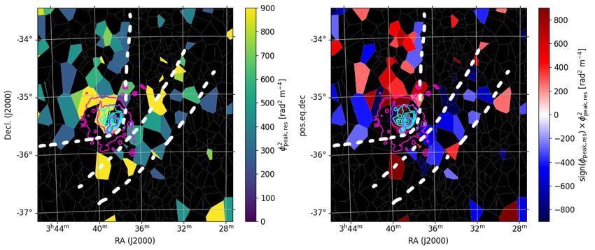
The morphology of the φpeak,res enhancement is revealed in Burn, 1966; Murgia et al., 2004; Bonafede et al., 2011). A
Figure 8, where we interpolate (using the nearest neighbour 2-sample Kolmogorov–Smirnov test comparing the polarised
method) and plot φ2peak,res as a function of position. Contours intensity distribution of our sample inside versus outside 1
showing the observable extent of the X-ray-emitting ICM as degree results in a D-value of 0.22 with a p-value of 0.001,
seen by Chandra (Scharf et al., 2005) and ROSAT (Jones et al., suggesting the lower apparent polarised flux near the cluster
1997) are overlaid, as are contours for the radio galaxy Fornax is statistically significant at the ∼ 3.3σ level. The question
A (see Norris et al. submitted). We note that the Chandra and is then whether sources near the cluster are fewer, fainter, or
ROSAT X-ray maps are smoothed to 2.5 and 3 arcminutes both, and whether depolarisation or some other mechanism
respectively to reveal the faint diffuse emission. Particularly is responsible for this.
for the ROSAT contours, the apparent degree of extension We investigated this by calculating the polarised source
towards the southwest is affected by the smoothing required counts, and the integrated and median polarised and total flux,
combined with the presence of bright point sources unrelated in equal-area (π-square degrees) annular bins centred on NGC
to the cluster medium. The ICM is therefore more asymmetric 1399. The experiment is described in more detail in Appendix
around NGC 1399 — more ‘swept back’ towards northeast B, while the results are shown in Figure 10. The polarised
— than the ROSAT contours initially seem to imply (echoing source counts (top panel of Figure 10) show a 2σ decrement
the morphology of the Chandra contours). The dispersion in inside one degree radius (averaging 17 polarised sources per
φpeak,res is clearly enhanced in the vicinity of the main cluster, square degree), a 2σ enhancement between 1 and 2 degrees
extending to a radius of one degree in most directions, and to radius (averaging 34 polarised sources per square degree),
1.5–2 degrees towards the N and NW. The radial extent of the but are consistent with our average 27 polarised sources per
enhanced region exceeds that of the currently observable X- square degree thereafter. Taken on their own, these deviations
ray emitting ICM by a factor of 2–4 depending on azimuthal are not statistically significant in a sky area the size of our
bearing, but lies within the 1.96 degree (705 kpc) virial radius mosaic. However, the plots of the integrated and median flux
of the cluster (Iodice et al., 2017; indicated on Fig. 8). densities (middle and lower panels of Figure 10, respectively)
The global φpeak,res enhancement appears to be comprised mirror the behaviour of the source count plot, and here the
of two smaller sub-regions: the first, a circular sector of angle deviations are significant. The integrated polarised and total
∼ 90◦ , with its vertex located near NGC 1399, and its two fluxes (respectively) show ∼ 3σ and ∼ 2σ decrements relative
enclosing radii oriented slightly clockwise of N-S and E-W to the expectation from the broader mosaic inside 1 degree
(respectively), and the second region, a ∼ 0.5◦ -wide strip radius, corresponding to a 50% decrement in polarised flux
centred ∼ 0.75◦ SW of NGC 1399, slightly concave towards in the former case. The data then show a ∼ 2.5σ and ∼ 4σ
it. The sharp decline in φpeak,res dispersion at 1 degree cluster- enhancement in the integrated polarised and total flux (respec-
centric radius is particularly evident at the outer edge of this tively) between 1 and 2 degrees radius. In total intensity only,
feature. This ‘two region’ interpretation is bolstered when the enhancement continues to fall outside the 99.7% confi-
the sign of the φpeak,res values are considered (see Figure 9). dence interval until a radius of 2.3 degrees, beyond which it
The SW enhancement shows predominantly negative φpeak,res returns to low-significance deviations from the expectation
values, indicating that the magnetic field in this structure is value, along with the polarised flux. The median polarised and
oriented predominantly away from the observer. Conversely, total fluxes also show ∼ 2.5σ and ∼ 3σ decrements (respec-
the NE enhancement does not reveal an obvious bias towards tively) inside 1 degree radius, but less significant deviations
either positive or negative values, implying that the magnetic in other bins. This may indicate that the flux decrement inside
field in this region is more isotropic. 1 degree is driven by the bulk of the sources therein, while
We note the existence of another possible region of en- the flux enhancement from 1–2.3 degrees may be driven by
hanced φpeak,res dispersion, which runs adjacent to the Fornax a smaller proportion of brighter sources. Finally, the median
A lobes to their NE, and which is not obviously attributable fractional polarisation shows no evidence for a decrement at
to calibration or image artifacts. While comprised of only small cluster-centric radii, as was found by Bonafede et al.
six sources, the φ2peak,res values are clearly elevated above (2011) for a sample of clusters, who attributed the effect to
the typical surrounding values for field sources — values depolarisation by turbulent cells in the ICM as per our mo-12 C. S. Anderson et al.
Projected distance from NGC 1399 [deg]
0.0 1.4 2.8 4.2
+60
+40
+20
[rad m 2]
0.0
peak, res
-20.0
-40.0
-60.0
0 200 400 600 800 1000 1200 1400
0
5
0
5
0
Projected distance from NGC 1399 [kpc] 0.0
0.2
0.5
0.7
1.0
CDF (Normalized)
Figure 6. Foreground-corrected Faraday depth (φpeak,res ) versus projected distance from NGC 1399. The foreground was removed as described in Section 5.1.
Data points within one degree (indicated by the red shaded region) show an excess dispersion, as described in Section 5.1. Sources that are located inside the
Fornax cluster volume, instead of behind it, are indicated with magenta crosses (see Section 4). Note that all such sources are in fact sub-components of the
central radio source in NGC 1399 (following from our approach for dealing with heavily resolved sources, discussed in Section 3).
The blue step plot shows the half-interdecile range (i.e. the interdecile range divided by two) for the data points located within
each 0.56 degree (200 kpc) -wide step. The vertical blue bars indicate the associated 90% confidence interval for the
underlying population distribution in each bin, calculated using bootstrap re-sampling. The right-most axes show normalised
cumulative histograms of φpeak for sources located within (red) and outside (black) a projected distance of one degree. The red
shading highlights the difference between these distributions.Fornax cluster magnetic fields 13
intensity data from GLEAM and NVSS track the ASKAP
20 data closely, as does the polarised intensity data from NVSS,
peak, res| [rad m 2]
ruling out instrumental effects. A final question is whether
15 these effects are observed over a range of flux densities. In
Figure 11, we plot the normalised integrated source counts
10 versus flux density, which we calculate both inside and out-
side 1 degree cluster-centric radius, for both polarised and
Median |
total intensity. The data show that the decrement inside 1
5 degree radius persists over a wide range in flux density.
Thus, we draw the following conclusions: (1) the polarised
0 source counts, the polarised flux densities, and the total flux
0 1 2 3 4
Projected distance from NGC 1399 [deg] densities all show decrements inside 1 degree projected radius
from the cluster; (2) the average magnitude of the decrement
Figure 7. The median of |φpeak,res | in a sliding window of width 0.5 degrees is ∼ 50% for the polarised flux, and ∼ 30% for the total
as a function of the cluster-centric radius of the outer bound of this window intensity; (3) between 1 and 2.3 degrees projected radius,
(blue line). The blue-shaded region indicates
√ the 95% confidence interval on there is a surfeit of flux in one or both quantities; (4) none
this value, calculated as ±1.58 × IQR/ n (McGill et al., 1978), where IQR
and n are the interquartile range and number of measurements (respectively) of these results can be attributed to a normalisation problem,
of |φpeak,res | in the sliding window. A sharp and significant decrease in the instrumental effect, or the modest ∼ 50% increase in image
plotted values is evident when the outer bound of the window passes a noise that occurs in a small ∼ 20 × 10 arcminute region
cluster-centric radius of 1 degree, which is marked with a vertical red dashed around PKS B0336–35 (see Figure 3 and Section 3); (5) the
line. The width of the sliding window is indicated by the gray shaded region.
coexistent decrements in Stokes I and P are inconsistent with
our initial hypothesis that depolarisation by turbulent cells in
the Fornax ICM could cause the decrement in P (cf. Bonafede
tivating hypothesis above. Instead, we find that the median et al., 2011). We discuss these results further in Section 6.7.
fractional polarisation is ∼ 5%, which is consistent with the
values that Bonafede et al. (2011) derive at cluster-centric
distances larger than 1.5 effective core radii (see figure 2 of 5.3 Summary of observational results
that work). However, this comparison comes with the caveats
that (a) our polarised sources at small cluster-centric radii is We summarise our observational results as follows:
insufficient to probe the core ICM regions where Bonafede
et al. (2011) observed the depolarisation effect, and (b) our • The distribution of peak Faraday depths for discrete
RM grid sources are confirmed to lie exclusively behind the radio sources shows an excess scatter of σφpeak,res,cluster =
Fornax cluster, whereas Bonafede et al. (2011)’s sample was 16.8 ± 2.4 rad m−2 within 1 degree (360 kpc) of the
a heterogeneous mixture of sources embedded in the clusters Fornax cluster centre. In more spatially-limited areas,
being measured, as well as in the background (though see the excess can be traced out to the ∼ 1.96 degree (705
their Appendix A.1 for arguments that this cannot explain kpc) virial radius of the cluster.
their results). In the future, it might be possible to probe closer • The projected area of the Faraday depth enhancement
to the core of the Fornax cluster using the central radio source extends 2–4 times the projected distance of the X-ray
hosted in NGC 1399 (e.g. Killeen et al., 1988), at which point emitting ICM, though is mostly contained within the
a more detailed comparison would be appropriate. cluster’s virial radius.
We note that the decrement and enhancement structures • The global Faraday depth enhancement naturally divides
described above are visually apparent in Figure 3 (in polari- into two distinct (projected) morphological sub-regions:
sation). The results are unusual for the Stokes I emission in (1) A triangular region extending from its vertex near
particular, for it is not obvious how emission or transmission NGC 1399 towards its apparent base about ∼ 1.5◦ to the
processes linked to the cluster could produce them (see dis- NE, with a mix of both positive and negative φpeak,res
cussion in Section 6.7). A mundane possibility is that, given values, and (2) a banana-shaped strip of width ∼ 0.5◦
the fact that the data were collected during ASKAP’s Early and length ∼ 2.5◦ , curving slightly around NGC 1399,
Science phase, the effect could be instrumental. We rule this but centred ∼ 0.75◦ to its SW, and having predominantly
out conclusively by including data from the GaLactic and negative φpeak,res values.
Extragalactic All-sky Murchison Widefield Array (GLEAM; • On average, the areal total and polarised radio emission
72–231 MHz; Wayth et al., 2015; Hurley-Walker et al., 2017) density is ∼ 30% and ∼ 50% lower within 1 degree
and NVSS (1.4 GHz; Condon et al., 1998) survey catalogues (360 kpc) of the Fornax cluster (respectively) compared
in the middle panel of Figure 10. We applied the same spatial to outside this radius. Cumulative source counts versus
truncations to these data as to our sample, and then scaled flux density show that the emission decrement persists
their fluxes to those expected in the ASKAP band assum- over the full range of flux densities that are effectively
ing a spectral index of −0.7. Evidently, the modified total probed by our observations and sample.You can also read