EMI Debugging with the R&SRTO and R&SRTE Oscilloscopes Application Note
←
→
Page content transcription
If your browser does not render page correctly, please read the page content below
EMI Debugging with the R&S®RTO
and R&S®RTE Oscilloscopes
Application Note
Products:
         ®
ı   R&S RTO
         ®
ı   R&S RTE

This application note offers a straightforward
description of how to analyze EMI problems using
           ®                ®
the R&S RTO and R&S RTE. The discussion
begins by covering the basic mechanisms that can
result in unwanted RF emissions and then describes
how to proceed in analyzing EMI problems. Finally,
a practical example is given to illustrate the analysis
process.

                                                                                 Dr. Markus Herdin
                                                                             6.2014 – 1TD05 – 1.1e
                                                          Application Note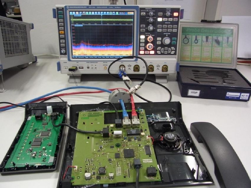
Table of Contents

               Contents
          1 Introduction ......................................................................................... 4

          2 Basic Principles of Radiated Emissions ........................................... 5
        2.1    Interference Sources ...................................................................................................5
       2.1.1   Differential-Mode RF Emissions ....................................................................................6
       2.1.2   Common-Mode RF Emissions .......................................................................................7
       2.1.3   Conducted Emissions ..................................................................................................10
       2.1.4   Signal Integrity Problems as an Interference Source ..................................................11
        2.2    Coupling Mechanisms ...............................................................................................12
        2.3    Emitting Elements (Antennas)..................................................................................12

          3 Measurement Methods for Use in EMI Debugging......................... 14
        3.1    Introduction – Near Field and Far Field ...................................................................14
        3.2    RFI Current and Voltage Measurements .................................................................15
       3.2.1   Relationship between RFI Currents on Connected Lines and Emitted Far-Field
               Components.................................................................................................................15
       3.2.2   How to Utilize RFI Current Measurements ..................................................................15
       3.2.3   Measurement of RFI Voltages on Power Lines ...........................................................16
       3.2.4   Current Probes for Measuring RFI Currents ................................................................17
        3.3    Analysis of EMI Problems Using Near-Field Probes ..............................................18
       3.3.1   Electric and Magnetic Near-Field Probes ....................................................................18
       3.3.2   Applications for Near-Field Probes ..............................................................................20
                            ®
       3.3.3   The R&S HZ-15 Near-Field Probe Set........................................................................22

          4 Practical Aspects of EMI Debugging with the R&S®RTO Digital
            Oscilloscope ..................................................................................... 23
        4.1    Basic Procedure for EMI Debugging in Development Labs ..................................23
                                     ®
        4.2    Using the R&S RTO for EMI Debugging .................................................................24
       4.2.1   Basic Oscilloscope Settings .........................................................................................24
                                 ®
       4.2.2   Special R&S RTO Functions for EMI Debugging .......................................................25
                                                                                 ®
       4.2.3   Tips & Tricks for EMI Debugging with the R&S RTO..................................................30
        4.3    Practical Example ‒ EMI Debugging on an IP Telephone......................................31
       4.3.1   Results of the Far-Field Analysis .................................................................................32
       4.3.2   RFI Current Measurement on the Connected Lines ....................................................33
       4.3.3   Near-Field Analysis ......................................................................................................37
       4.3.4   Result of the EMI Debugging .......................................................................................44

1.1e                        Rohde & Schwarz EMI Debugging with the R&S®RTO and R&S®RTE Oscilloscopes                                          2
Table of Contents

       5 Summary ........................................................................................... 45

       6 References ........................................................................................ 46

       7 Ordering information ........................................................................ 47

1.1e                  Rohde & Schwarz EMI Debugging with the R&S®RTO and R&S®RTE Oscilloscopes                    3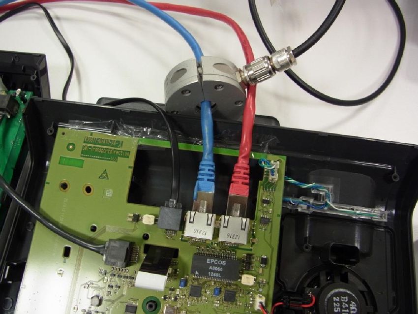
Introduction

       1 Introduction
         To some extent, all electric as well as electronic devices emit unwanted
         electromagnetic fields and transmit unwanted disturbance voltages and currents via
         their connection lines. In order to prevent such electromagnetic interference affecting
         the operation or radio reception of other devices, legal limits for emissions are
         stipulated by law in every economic region.
         EMC conformity tests are used to verify compliance with required limits. Time-
         consuming debugging is typically required in case of noncompliance. Prompt analysis
         of EMI problems starting in development is a key success factor for products that need
         to be launched onto the market in due time.
                                                ®                ®
         The powerful FFT function in the R&S RTO and R&S RTE digital oscilloscopes from
         Rohde & Schwarz allows analysis of EMI problems right at the developer's own
         workplace. With their 1 mV/div sensitivity, up to 4 GHz bandwidth and very low input
         noise, these oscilloscopes are a very useful tool in this application. Developers can use
         near-field probes as well as current probes to localize and analyze unwanted radiated
         emissions and disturbance currents and develop efficient solutions to reduce them.
         This application note provides a simple guideline to help hardware developers analyze
         EMI problems using near-field probes in conjunction with digital oscilloscopes. The
         actual analysis process is demonstrated based on a practical example using the
             ®
         R&S RTO.

1.1e              Rohde & Schwarz EMI Debugging with the R&S®RTO and R&S®RTE Oscilloscopes       4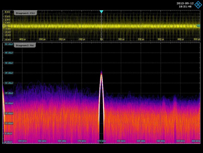
Basic Principles of Radiated Emissions

        2 Basic Principles of Radiated Emissions
           As a basic rule, radiated emissions can occur only when the following conditions are
           fulfilled:
           a) An interference source exists that generates a sufficiently high disturbance level in a
           frequency range that is relevant for RF emissions (e.g. fast switching edges)
           b) There is a coupling mechanism that transmits the generated disturbance signals
           from the interference source to the emitting element
           c) There is some emitting element that is capable of radiating the energy produced by
           the source into the far field (e.g. a connected cable, slots in the enclosure or a printed
           circuit board that acts as an antenna)
           We will consider all three of these elements in the following section.

       2.1 Interference Sources
           Modern digital circuits use square-wave signals at high frequencies with steep rise and
           fall times in order to transmit digital information. Single-ended (asymmetrical) signal
           transmission (e.g. parallel address or data buses) is typically used between the
           different components, although differential (symmetrical) transmission is also used in
           case of very high clock speeds (e.g. differential clock lines). Such devices generate
           electromagnetic energy with a high-frequency spectrum that is capable of being
           radiated. Due to the technology used, the circuit components have low supply voltages
           and are therefore at the same time sensitive to electromagnetic disturbance affecting
           the system from outside, e.g. via the power supply network.
           Parts of a circuit, such as switched mode voltage converters that rely on switching
           operations with steep edges, can also act as an interference source with a number of
           high-frequency harmonics.

1.1e                Rohde & Schwarz EMI Debugging with the R&S®RTO and R&S®RTE Oscilloscopes        5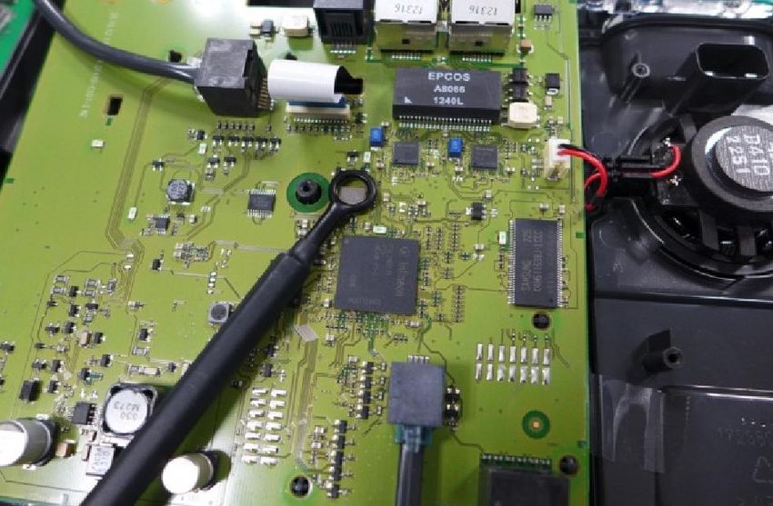
Basic Principles of Radiated Emissions

             Fig. 2-1: Square-wave signal with odd harmonics.

             Although the amplitude of the harmonics decreases with frequency (20 dB per decade
             for square-wave signals, 40 dB per decade above a certain cutoff frequency for signals
             with a finite rise time), harmonics play an important role in unwanted radiated
             emissions. At higher frequencies, disturbance signals are radiated more efficiently
             because the conductor structures used in electronic systems begin to reach the order
             of the wavelength of the disturbance signals (see section 2.1.2). For this reason, when
             using switched mode power supplies, it is typical to first see the high harmonics as a
             disturbance spectrum in the far field, for example.
             In the case of unshielded systems, the actual emission of the interference into the far
             field occurs, for example, directly via the tracks or components on the printed circuit
             board. In the case of shielded systems, unwanted RF emissions can occur due to
             openings in the shielded enclosure or due to an RFI current that is coupled onto a
             connected cable.

       2.1.1 Differential-Mode RF Emissions

             Differential-mode RF emissions from printed circuit boards occur due to the flow of
             current (IDM) via signal paths in which the forward and return conductors are not routed
             together, thereby forming a conductor loop. In this case, the interference source is a
             result of the circuit's primary function, i.e. transferring data between two components of
             the circuit. The EMI problem is caused by inappropriate arrangement of the tracks. The
             resulting magnetic field from the conductor loop is proportional to the current IDM, the
             area of the loop and the square of the frequency of the RFI current.

1.1e                   Rohde & Schwarz EMI Debugging with the R&S®RTO and R&S®RTE Oscilloscopes       6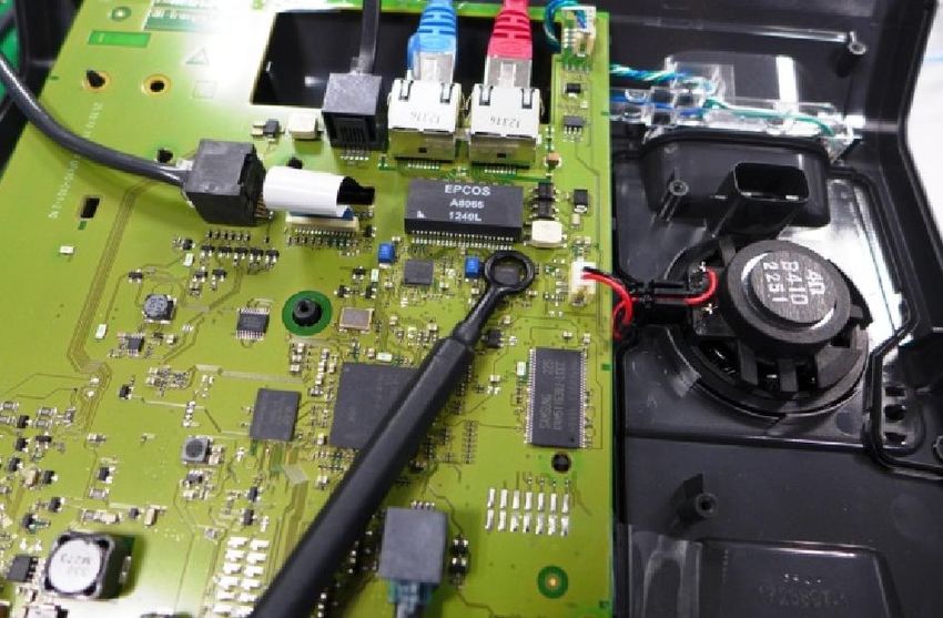
Basic Principles of Radiated Emissions

            Fig. 2-2: Differential-mode RF emissions from printed circuit boards and positioning of loop near-
            field probes for measuring such emissions.

            Near-field test equipment can be used to detect sources of differential-mode RF
            emissions. Here, we use loop antennas with appropriate directivity, and the loop
            antenna must be rotated during the measurement in order to find the maximum value
            of the RF emissions. This is especially important for comparison measurements after
            taking corrective measures to eliminate the interference since the radiation pattern can
            be affected by such measures. Furthermore, the magnetic near field drops off sharply
            with distance. This makes it important to record the measured values at the exact
            same location.
            Steps that can reduce differential-mode RF emissions include reduction of the loop
            area (i.e. closer routing of the forward and return conductors) as well as reduction of
            the current in the conductor loop if this is possible without impacting the circuit's
            operation. Another alternative, for example, is to reduce the rise/fall times for the
            transmitted data signals or use filtering to eliminate higher-frequency signal
            components and thus limit the disturbance spectrum.

       2.1.2 Common-Mode RF Emissions

            Common-mode RF emissions occur due to undesired parasitic effects, e.g. due to
            inductances in the current return path or unsymmetries during signal transmission. This
            problem is very common with multilayer printed circuit boards in cases where slots or
            other discontinuities in the ground plane prevent the return current for transmitted
            signals from flowing close to the signal line. This leads to an undesired inductance in
            the path of the return signal and thus to unwanted voltage differences between

1.1e                  Rohde & Schwarz EMI Debugging with the R&S®RTO and R&S®RTE Oscilloscopes              7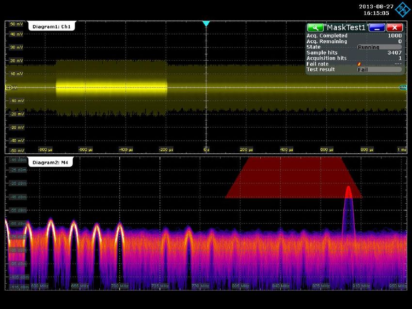
Basic Principles of Radiated Emissions

       different points in the ground plane. If we connect a cable to a printed circuit board of
       this type, it will function like an antenna and allow a common-mode current ICM to flow.
       In the frequency range relevant for RF emissions, signal and power supply lines can
       function as very efficient antennas. Here, our rule of thumb is that line lengths that do
       not exceed λ/10 are uncritical, whereas longer lines (e.g. λ/6) must be treated as
       potential sources of RF emissions.

       Fig. 2-3: Common-mode RF emissions from a printed circuit board. The source is a slot in the ground
       plane which causes a parasitic inductance in the return conductor. This causes a voltage drop
       between different points in the ground plane.

       The magnitude of the voltage drop on the ground plane and thus the magnitude of the
       common-mode current coupled into the connected line are determined by the parasitic
       inductance and the slope steepness of the signal. Common-mode RF emissions can
       therefore be reduced by limiting the rise and fall times (i.e. the frequency spectrum)
       and reducing the impedance in the ground plane. Since we are typically unable to
       sufficiently reduce the slope steepness for high-speed digital signals without incurring a
       loss of functionality, the handling of the return current (path with lowest possible
       inductance) is a critical element in the design process.

1.1e             Rohde & Schwarz EMI Debugging with the R&S®RTO and R&S®RTE Oscilloscopes               8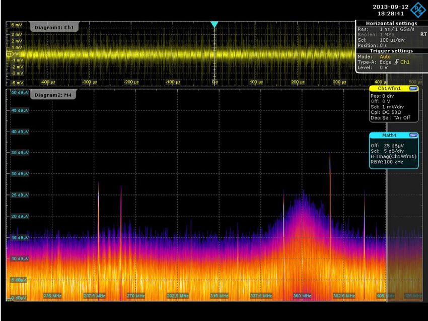
Basic Principles of Radiated Emissions

       Fig. 2-4: Ideal differential-mode transmission: The forward and return conductors are arranged close
       to one another while the generated magnetic field is almost entirely canceled out in the far field.

       Fig. 2-5: Formation of a common-mode return current via the antenna path due to undesired parasitic
       inductance in the ground plane. Here, the "antenna path" is typically an external line that functions
       as an antenna, e.g. a power supply cable.

       In actual practice, common-mode RF emissions can also occur due to differential-
       mode signal transmission. If the parasitic terminating impedances of a differential-
       mode transmission path differ substantially, in addition to the desired differential-mode
       current IDM a common-mode current ICM will also flow via the ground plane that
       connects the transmitter and receiver modules. This unwanted ground current ICM can
       then also be coupled into lines connected to the board and cause emissions in the far
       field.

1.1e              Rohde & Schwarz EMI Debugging with the R&S®RTO and R&S®RTE Oscilloscopes                9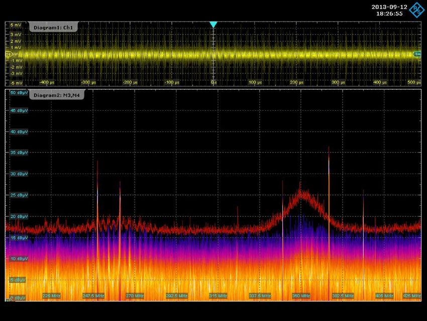
Basic Principles of Radiated Emissions

            Fig. 2-6: Unbalanced (parasitic) terminating impedances of a differential-mode signal line that causes
            an unwanted common-mode current ICM. A line connected to the ground plane can thus function as
            an antenna if it is capable of carrying a part of the common-mode current ICM.

            In practice, common-mode currents are one of the main causes of undesired RF
            emissions. Near-field test equipment can be used to detect sources of common-mode
            RF emissions. Magnetic near-field probes that are capable of detecting common-mode
            current (or the resulting field) are suitable for this task. Using compact near-field
                                                                   ®
            probes such as the RS-H 2.5-2 included in the R&S HZ-15 near-field probe set (see
            section 3.3.3) for determining the current in individual tracks, it is possible to calculate
            the actual common-mode RFI current using a conversion factor. Of course, the near-
            field measurements must be supplemented with measurements of the common-mode
            current along the connected lines.

            General steps to help reduce common-mode RF emissions:
            ı   Reduce the RFI current ICM by optimizing the layout, reducing the ground plane
                impedances or rearranging components
            ı   Reduce higher-frequency signal components through filtering or by reducing the
                rise and fall times of digital signals
            ı   Use shielding (lines, enclosures, etc.)
            ı   Optimize the signal integrity to reduce unwanted overshoots (ringing), see also
                section 2.1.4

       2.1.3 Conducted Emissions

            The lines connected to a device are often the primary source of RF emissions.
            Electromagnetic waves in the frequency range from 30 MHz to 1 GHz have
            wavelengths from 10 m to 30 cm. Cables can thus efficiently radiate an RFI current
            (see section 2.1.2) since their length is in the range of these wavelengths in standard
            test setups required for far-field measurements.
            Radiation of common-mode currents is especially efficient. Although the fields that
            arise along the cable due to differential-mode currents cancel out partially, this is not
            the case for common-mode currents. The radiated field strength is directly proportional
            to the common-mode current.

1.1e                   Rohde & Schwarz EMI Debugging with the R&S®RTO and R&S®RTE Oscilloscopes                10
Basic Principles of Radiated Emissions
Near-field measurements can be used to detect the interference sources. By
measuring the RFI current on the lines connected to the DUT, we can ascertain
whether a connected line is causing RF emissions into the far field.
RF current probes are used to measure the common-mode current and are available in
different versions (for different cable diameters and frequency ranges). During these
measurements, it should be taken into account that the RFI current varies as a function
of its position on the line.
2.1.4 Signal Integrity Problems as an Interference Source
When transmitting signals with high slope steepness, it is no longer reasonable to
neglect the propagation velocity, i.e. the time required for the signal to travel from the
transmitter to the receiver. Impedance mismatches on the transmission path cause
reflections, where part of the signal wavefront returns to the source and is
superimposed on the original signal.
When digital signals are transmitted, this effect leads to ringing artifacts and thus to the
formation of disturbance signals which can be emitted. All of the components along the
transmission path (e.g. transmitter, track, cable, connector, receiver) must be matched
to the relevant characteristic impedance in order to ensure proper signal integrity as an
essential prerequisite to achieving EMC compliance.
If the signal integrity is inadequate, we can analyze the problem by measuring the
signals, e.g. at the transmitter output or the receiver input. After conversion to the
frequency domain by means of an FFT, the spectrum of the interference source can be
compared to the result of a far-field measurement in order to determine the
corresponding source.
Fig. 2-7: PSpice simulation of ringing: transmission of a clock signal with 0.5 ns rise time/fall time
and 20 ns pulse width via a 100 unterminated line; propagation time on the line: 0.1 ns; source
impedance of transmitter: 10 . (Red) transmitted clock signal; (blue) signal at transmitter output;
(green) signal at receiver.
1.1e Rohde & Schwarz EMI Debugging with the R&S®RTO and R&S®RTE Oscilloscopes 11Basic Principles of Radiated Emissions
2.2 Coupling Mechanisms
For interference generated on a printed circuit board to be emitted, the RFI power must
be transferred from the source to the emitting element. This is known as the "coupling
path" and the transmission type is referred to as "coupling mechanism".
We basically distinguish between the following coupling paths:
1. Direct RF emissions from the source, e.g. from a track or an individual
component
2. RF emissions via connected power supply, data or signal lines
3. Conducted emission via connected power supply, data or signal lines
Potential coupling mechanisms are as follows:
1. Coupling via a common impedance
In this case, the interference source and emitting element are connected via a
common impedance.
This situation occurs frequently since a direct connection usually exists in
electronic systems between an interference source and an emitting element
(e.g. the common ground of an affected digital circuit (interference source) and
the cable screen or ground conductor of a connected signal cable (antenna)).
2. Coupling via fields
a. Electric field
In this case, an electric near field is generated emitted by the interference
source. This field is coupled into an adjacent circuit or an emitting element
(e.g. heat sink) and then radiated into the far field or emitted in a
conducted manner. The parasitic coupling capacitance between the
interference source and sink influences the energy transfer as a function of
frequency.
b. Magnetic field
In this case, an electric circuit produces a magnetic near field, which
couples into an adjacent conductor loop or a magnetically sensitive
component. The resulting energy transfer is determined by the coupling
coefficient between the circuits and the current in the interference source.
c. Electromagnetic field
In this case, the interference source and sink are far apart, i.e. at least one
λ or a multiple thereof. Both an electric field and a magnetic field are
generated. The source emits the interference directly into the far field.
2.3 Emitting Elements (Antennas)
The emitting elements that are relevant in EMI applications are basically unintentional
antennas.
1.1e Rohde & Schwarz EMI Debugging with the R&S®RTO and R&S®RTE Oscilloscopes 12Basic Principles of Radiated Emissions
The efficiency of such antennas (radiation resistance, antenna factor) depends on the
geometry of the antenna. The main factor is the length of the antenna with respect to
the wavelength of the interference.
Antennas with lengths of only a fraction of the interference wavelength, e.g. λ/6, can be
efficient radiators. The rule of thumb here is that antennas with a length less than λ/10
are not critical.
The following are the main types of unintentional antennas in electronic equipment:
ı Connected lines (power supply, data/signal/control lines)
ı Printed circuit board tracks and planes
ı Internal cables between system components
ı Components and heat sinks
ı Slots and openings in enclosures
1.1e Rohde & Schwarz EMI Debugging with the R&S®RTO and R&S®RTE Oscilloscopes 13Measurement Methods for Use in EMI Debugging
3 Measurement Methods for Use in EMI
Debugging
3.1 Introduction – Near Field and Far Field
In EMC compliance testing, we really only care about the DUT's emissions into the far
field. We use the term "far field" if the electric and magnetic field components are in
phase and oriented perpendicular to the direction of propagation and a plane wavefront
has formed. The electromagnetic wave has separated from the antenna and is now
dependent on the propagation conditions in the medium (as opposed to the
characteristics of the source). For radiators that are small with respect to wavelength,
the far field begins at a distance of about λ / 2π, while for antennas that are large with
respect to wavelength, it does not begin until 2 ∙ D / λ. Here, D is the diameter of the
antenna structure.
The far-field measurements required in regulatory compliance testing are feasible only
in specialized EMC test labs (test chambers or open-area test sites) and tend to be
costly and time-consuming. When problems occur with EMC compliance, cost and time
limitations typically prevent multiple visits to the test lab in order to develop and
analyze improvements. However, other measurement methods do exist that can be
used to analyze EMI problems. For applications in development labs, near-field and
RFI current measurements are an attractive alternative.
The near field comprises electric and magnetic field components that drop off by a
factor of 1 / r or 1 / r with distance. In EMC compliance testing, only the far field is
relevant; it drops off proportional to 1 / r as the distance from the source increases. In
the near field, the electric and magnetic field components are not yet tied to the
characteristic wave impedance of free space (377 Ω). The wave is not yet
disconnected from the transmitter and the field components still depend on the
characteristics of the source. For this reason, we cannot draw any conclusion about
the far field (and thus EMC compliance) from levels we measure in the near field.
However, the opposite conclusion is possible: If we can measure electromagnetic
waves in the far field, then electric as well as magnetic field components must be
present in the near field. For example, if we determine during an EMC compliance test
that the DUT is producing unacceptable levels of radiation, we can use near-field
probes to locate the source of such emissions.
When interpreting results delivered by a near-field probe, we must always take into
account whether relevant antenna structures (e.g. connected cables or long tracks) are
present that radiate into the far field. Near-field emissions with high amplitudes need
not necessarily lead to strong far-field emissions.
In addition to near-field measurements, it is also important to measure the RFI currents
that flow, for example, on connected signal or power supply cables of the DUT in order
to analyze the cause of RF emissions.
1.1e Rohde & Schwarz EMI Debugging with the R&S®RTO and R&S®RTE Oscilloscopes 14Measurement Methods for Use in EMI Debugging
As a general rule, it is recommended to perform a far-field measurement in order to
identify the critical frequencies prior to analysis with near-field probes. The actual
interference sources can then be localized with a near-field measurement. Once the
coupling mechanism into the far field has been identified, suitable corrective action can
be taken to eliminate the problem.
3.2 RFI Current and Voltage Measurements
3.2.1 Relationship between RFI Currents on Connected Lines and
Emitted Far-Field Components
A typical radiation mechanism involves common-mode RFI currents that flow on the
inside conductor or the screen of lines connected to the DUT. Because such lines
usually have a length of at least one meter, they represent efficient antennas in the
frequency range from 30 MHz to 1 GHz which is highly relevant in EMC compliance.
As such, they are often the most critical emitting element. The resulting field strength in
the far field is directly proportional to the RFI current; steps to reduce this current thus
lead to a direct improvement in radiated emissions. The following formula [1]
[ / ]=4∙ ∙ 10 ∙ [ ]∙ [ ]∙ [ ]∙ (Θ) /
provides a simple estimate of the maximum permissible common-mode RFI current on
connected lines (based on the assumption of a dipole antenna). Here, l is the line
length, r is the distance between the source and receiving antenna, Icm is the common-
mode RFI current and is the angle with respect to the dipole.
For an angle = 90°, a measurement distance of 3 m, a frequency of 100 MHz, a
cable length of 1 m and an RFI current of 2.5 μA, an RF emission field strength level of
about 100 μV/m (= 40 dBμV/m) is obtained. For example, this corresponds to the Class
B limit in line with EN55022. It is thus clear that even RFI currents on the order of
2.5 μA can violate EMC compliance limits.
3.2.2 How to Utilize RFI Current Measurements
By measuring the common-mode current on the lines connected to the DUT, we can
determine whether any lines produce emissions present in the far field and if so, what
lines. If the RFI currents are negligible on all connected lines, then another mechanism
must be responsible for RF emissions (e.g. RF leakage through the enclosure due to
insufficient RF shielding).
Moreover, by comparing the spectrum of the RFI current with the measured spectrum
in the far field, we can determine the main interference source on the printed circuit
board. For example, if a broadband interferer is present in the far field with a maximum
value at 100 MHz and an interferer with a similar spectrum is detected in the near field,
we have obviously found the source of the interference in the near field. CW interferers
can be treated analogously. For example, if harmonics of 25 MHz are present in the far
field and an interference source is detected in the near field with a comparable
harmonic spectrum, it is most likely the interference source we are seeking.
1.1e Rohde & Schwarz EMI Debugging with the R&S®RTO and R&S®RTE Oscilloscopes 15Measurement Methods for Use in EMI Debugging
Due to the direct proportionality between the electromagnetic waves emitted into the
far field and the RFI current, proposed improvements are easy to evaluate.
Reproducible measurement conditions are a critical element of such comparison
measurements. It is important to pay special attention to the fact that the RFI current
varies as a function of its position on the line. Due to reflections on the connected line,
standing waves can arise which lead to different RFI currents at different locations on
the line. In order to be able to measure the resulting improvement in far-field
emissions, a current probe (see section 3.2.4) must be used to measure the maximum
RFI current on the line (e.g. a power line). The line length should not be changed
during the procedure. In addition, problematic standing waves can be attenuated using
absorbing clamps (ferrites) on the end of the line if necessary.
Fig. 3-1: R&S®EZ-24 absorbing clamp for attenuation of standing waves during measurement of the
RFI current.
Generally, when measuring radiated emissions in development labs, it is important to
pay attention to whether the measured emissions could possibly represent ambient
interference. It is thus recommended to make a preliminary measurement with the DUT
switched off in order to isolate and measure the ambient interference.
3.2.3 Measurement of RFI Voltages on Power Lines
RFI voltage measurements are also used to determine the RFI current that propagates
along connected lines. Such measurements are performed on power lines using line
impedance stabilization networks (LISN), e.g. V-LISN on AC/DC power supply lines
and T-LISN on telecommunications lines. Line impedance stabilization networks are
intended to simulate the impedance of the power supply network or the cable
impedance, filter out extraneous interference from the connected power supply
network and make the RF interference generated by the DUT available at a
measurement output.
1.1e Rohde & Schwarz EMI Debugging with the R&S®RTO and R&S®RTE Oscilloscopes 16Measurement Methods for Use in EMI Debugging
Fig. 3-2: R&S®ENV216 two-line V-network for measuring conducted emissions
RFI voltage measurements can be used as a substitute for RFI current measurements
as well as for debugging in cases where excessive radiated emissions are occurring. It
is important to recall that line impedance stabilization networks are normally used for
frequency ranges below that of standard current probes.
3.2.4 Current Probes for Measuring RFI Currents
RF current probes are used to measure RFI currents and are available for different
cable diameters and frequency ranges. The following aspects are essential when
debugging EMI problems:
ı The inner diameter of the current probe should allow good magnetic coupling and
therefore needs to be matched to the cable diameter.
ı The frequency response should be as flat as possible in the frequency range of
interest.
ı The current probe's transfer impedance Z should be as high as possible in order
to display the measured current as an "amplified" output voltage V. The measured
current can then be easily calculated as follows: I [dBμA] = [ ]− [ Ω].
ı The current probe should be designed as a clamp so that it can be easily attached
around the line.
ı One example of a device suitable for RFI current measurements is the
®
Rohde & Schwarz R&S EZ-17 current probe with 20 Hz to 100 MHz bandwidth
and 10 dB (model 02) or 17 dB transfer impedance (model 03).
1.1e Rohde & Schwarz EMI Debugging with the R&S®RTO and R&S®RTE Oscilloscopes 17Measurement Methods for Use in EMI Debugging
Fig. 3-3: The R&S®EZ-17 current probe with 10 dBΩ transfer impedance (model 02) or 17 dBΩ transfer
impedance (model 03) and 20 Hz to 100 MHz bandwidth is a good example of a device suitable for
measuring RFI currents. The large inner diameter of 30 mm allows measurements on cable bundles.
®
For current measurements, absorbing clamps such as the R&S MDS-21 can also be
®
used, or ferrite clamps such as the R&S EZ-24 without a measurement output in
combination with any current probe that has adequate sensitivity and bandwidth along
with the appropriate diameter.
3.3 Analysis of EMI Problems Using Near-Field Probes
The main purpose of near-field probes is to measure the electric or magnetic field
produced by a DUT in a precisely defined area near the probe with the highest
possible sensitivity. Special shielding techniques are used in probes to suppress
unwanted fields from other directions. Furthermore, near-field probes are designed to
detect either magnetic or electric fields and to suppress the other field component as
much as possible. This allows detailed analysis of the relevant near field along with
pinpoint detection of interference sources. For example, there exist special near-field
probes that can be used to isolate and detect the emissions from individual tracks on a
printed circuit board. This allows identification of the track responsible for the radiated
emission to be examined. Other types of probes are specially designed to measure
currents in IC pins or in decoupling capacitors.
3.3.1 Electric and Magnetic Near-Field Probes
Electric near-field probes suppress the magnetic field component and produce an
output signal proportional to the electric field component (E) of the near field. Using a
frequency-dependent transducer factor (Ke), we can calculate the electric field strength
in the probe's near field as follows:
[ / ]= [ ]+ [ / ].
1.1e Rohde & Schwarz EMI Debugging with the R&S®RTO and R&S®RTE Oscilloscopes 18Measurement Methods for Use in EMI Debugging
Magnetic near-field probes suppress the electric field component and produce an
output signal proportional to the magnetic field component (H) of the near field. Using a
frequency-dependent transducer factor (Kh), we can calculate the magnetic field
strength as follows:
[ / ]= [ ] + ℎ[ /( )].
The magnetic near field is caused by an RF current. Using another transducer factor
(Ki) that is likewise frequency-dependent, we can estimate the current causing the field:
[ ]= [ ]+ [ / ].
The transducer factors are normally specified by the probe manufacturer. However,
they can also be determined independently based on a constant reference field.
Magnetic near-field probes in particular are typically not isotropic, i.e. the measured
field strength is dependent on the direction of the field, the selected position of the
probe and naturally the distance to the source. For this reason, the probe should be
placed directly on the relevant interference source (e.g. a track) and rotated until the
maximum value is measured for the field. This procedure increases the reproducibility
of repeat measurements, e.g. after undertaking steps to solve the problem.
Fig. 3-4: Formation / orientation of a magnetic near field caused by an RF current along a conductor.
In general, magnetic near-field probes have better interference immunity than electric
near-field probes, making them easier to use. Furthermore, both differential-mode as
well as common-mode RFI currents predominantly cause a magnetic near field and
can thus be detected with magnetic near-field probes. For this reason, measurements
using magnetic near-field probes represent the preferred diagnostic technique (in
addition to RFI current measurements on connected lines).
Electric near-field probes are used to perform comparative measurements of the
electric field, analyze and detect coupling mechanisms, and measure switching edges
on signal lines and in DC supply systems, to name some examples. They are
especially suited to applications where the emission is due primarily to changes in
electric potential (as opposed to electric currents). Moreover, they are often helpful
when looking for leaks in shielding enclosures.
1.1e Rohde & Schwarz EMI Debugging with the R&S®RTO and R&S®RTE Oscilloscopes 19Measurement Methods for Use in EMI Debugging
3.3.2 Applications for Near-Field Probes
Near-field probes are a useful tool for performing detailed analysis of EMI problems on
printed circuit boards. The main applications include localization of interference
sources and identification of decoupling mechanisms.
ı Localization of interference sources on printed circuit boards
Depending on the actual near-field probe used, the spatial region in which the
probe will detect electric or magnetic fields is necessarily small. By moving the
near-field probe over the DUT's printed circuit board, it is possible to determine at
which position a disturbance spectrum of interest has its maximum value. There,
we will often find the source of the interference that is causing a problem in the far
field. This can involve individual tracks, bus systems, power supply planes, ICs,
heat sinks and even switching transistors.
A near-field probe can also be used to study the current distribution in a ground
plane. In this manner, we can determine whether the return current is flowing via
the intended path or is unintentionally distributed due to breaks in the ground plane.
Probing decoupling capacitors provides a way to assess the effectiveness of power
supply decoupling measures. Using a magnetic near-field probe such as the RS-H
®
2.5 from the R&S HZ-15 near-field probe set, it is possible to measure the current
through the decoupling capacitor and understand how well it suppresses radiated
emissions. At higher current levels, the decoupling is generally more effective. By
choosing a different type of decoupling capacitor, changing its value and if
necessary modifying how it is connected in the layout to the power supply and
ground, we can maximize the measured current in the capacitor and thus optimize
its decoupling effect.
ı Identification of decoupling mechanisms
In combination with measurement of the RFI current on connected lines, near-field
probes can be used to clarify whether the measured near fields are coupled into
the far field via the connected lines. If this is not the case, near-field probing can be
performed around slots in the enclosure to determine whether inadequate shielding
is the cause of unwanted far-field emissions.
Once we have identified the interference sources and the decoupling mechanism, the
next step involves finding ways to solve the problem. This includes (for example):
ı Testing the signal integrity on critical transmission paths in the DUT. Typical
problems here include ringing, e.g. due to inappropriate termination of the
transmission lines
ı Reducing the slope steepness or filtering transmitted signals in order to reduce the
amplitude of the harmonics. Above a certain order, harmonics generally have no
substantial influence on the signal integrity but they are emitted more easily due to
their higher frequency
ı Modifying the layout e.g. optimizing the routing of the return current in cases where
single-ended (asymmetrical) signal transmission is used
1.1e Rohde & Schwarz EMI Debugging with the R&S®RTO and R&S®RTE Oscilloscopes 20Measurement Methods for Use in EMI Debugging
ı Reworking how power is supplied to critical components (power bus design)
ı Shielding and filtering lines, e.g. using SMD ferrites, common-mode chokes or
cable ferrites
ı Improving the shielding of the enclosure
1.1e Rohde & Schwarz EMI Debugging with the R&S®RTO and R&S®RTE Oscilloscopes 21Measurement Methods for Use in EMI Debugging
3.3.3 The R&S®HZ-15 Near-Field Probe Set
During analysis of EMI problems, a set of different near-field probes can be very
®
helpful. The R&S HZ-15 set contains two electric and three magnetic near-field probes
of different sizes that are ideal for this application.
RS-E 02: Large-area near-field probe for measuring electric fields
emitted from structures that have a larger surface area (e.g. address or
data buses, heat sinks, areas on printed circuit boards). Electric fields
are measured with the probe's bottom side; the top side is electrically
shielded. If possible, the entire probe should be placed on the DUT.
Measurement uncertainties due to an undefined distance between the
probe and source (or emitting element) can be reduced in this manner.
RS-E 10: Near-field probe with very high spatial selectivity for measuring
electric fields. The probe's shielding suppresses fields from adjacent
structures. Its resolution is approx. 0.2 mm, making it possible to locate
the tracks with the highest disturbance level in a group of tracks.
RS-H 400-1: Magnetic near-field probe with high sensitivity but relatively
low spatial selectivity. Very useful for performing an initial analysis in
cases requiring coarse measurement and localization of interferers. This
probe is directional and must be rotated during the measurement until
the maximum value is found.
RS-H 50-1: Magnetic near-field probe with significantly higher resolution
than the RS-H 400-1 but also significantly lower sensitivity. This probe is
directional and must be rotated during the measurement until the
maximum value is found.
RS-H 2.5: Magnetic near-field probe with high spatial resolution;
especially useful for measurement of RF currents in and along conductor
tracks, components and their leads as well as for detection of interferers
within bus systems. Can also be used to determine the current on the
surface of ICs or through capacitors. Consists of a core with a gap of 0.5
mm. The magnetic field is detected at the gap (white line). The probe is
placed with the gap directly on the interference source. This probe is
directional and must be rotated during the measurement until the
maximum value is found.
Table 3-1: R&S®HZ-15 near-field probe set.
1.1e Rohde & Schwarz EMI Debugging with the R&S®RTO and R&S®RTE Oscilloscopes 22Practical Aspects of EMI Debugging with the R&S®RTO Digital Oscilloscope
4 Practical Aspects of EMI Debugging with
the R&S®RTO Digital Oscilloscope
4.1 Basic Procedure for EMI Debugging in Development Labs
The following flowchart illustrates the basic procedure for EMI debugging. The process
is typically based on the results of a far-field measurement which provides a standard-
compliant summary of the critical frequencies.
Far-field measurement
provides standard-compliant EMC test lab
summary of critical
frequencies
Reference measurement with Development lab
DUT switched off to identify
extraneous radiated
emissions
RFI current measurement for
analysis of the emission
mechanism
Localization of the
interference source in the
near field and analysis of the
coupling mechanism
Evaluation of possible
corrective action
1.1e Rohde & Schwarz EMI Debugging with the R&S®RTO and R&S®RTE Oscilloscopes 23Practical Aspects of EMI Debugging with the R&S®RTO Digital Oscilloscope
The actual debugging process begins once the results from the far-field measurement
are available. The recommended procedure is as follows:
1. Reference measurement with DUT switched off to identify extraneous RF
emissions
Prior to beginning EMI debugging in the development lab, it is recommended to
perform a reference measurement with the DUT switched off. In this manner, we
can ensure that any RF emissions from other equipment in the lab or from radio
services will not be incorrectly identified as RF emissions from the DUT. This is a
crucial step when making measurements with electric near-field probes as well as
RFI current measurements on lines. Magnetic near-field probes are often immune
to extraneous RF emissions.
2. RFI current measurement if any lines are connected to the device
In many cases, lines connected to the device turn out to be the emitting elements
we are looking for. An RFI current measurement is used to determine which lines
are radiating the disturbance signal into the far field. Once the source has been
identified on the printed circuit board, the coupling mechanism can be tracked from
the interference source on the board to the emitting element. The coupling
mechanism is highly relevant when working to reduce the RF emissions.
3. Near-field measurement using different probes for locating the interference source
The best approach here is to begin with a large magnetic near-field probe such as
®
the RS-H 400-1 loop antenna (R&S HZ-15) and look for the interference source on
the printed circuit board. By then switching to smaller loop antennas such as the
RS-H 50-1 and the RS-H 2.5, we can further localize the interference source (see
page 22).
It is best to use magnetic near-field probes since they have better immunity to
undesired interference compared to electric near-field probes.
4. Analysis of possible corrective action
Once the interference sources, coupling mechanisms and emitting elements are
known, possible solutions can be implemented and analyzed. Near-field probes or
even current probes for RFI current measurements can be easily employed to
study the effect of the proposed solutions with respect to the RF emissions. Here, it
is important to always make comparison measurements with near-field probes at
the same point; the near-field probe must be rotated to detect the maximum value.
This is necessary since a potential solution can change the polarization of an RF
emission. During RFI current measurements on connected lines, it is likewise
important to always check for the local maximum of the RFI current.
4.2 Using the R&S®RTO for EMI Debugging
4.2.1 Basic Oscilloscope Settings
®
Use the following short steps to configure the R&S RTO for EMI debugging:
1.1e Rohde & Schwarz EMI Debugging with the R&S®RTO and R&S®RTE Oscilloscopes 24Practical Aspects of EMI Debugging with the R&S®RTO Digital Oscilloscope
ı Press PRESET to obtain a defined setup
ı Connect the current probe (for RFI current measurement) or the near-field probe
to any input channel
ı Select a vertical resolution in the range from 1 mV/div to 5 mV/div for high
sensitivity
ı Select 50 Ω coupling (for proper matching to the output impedance of the current
probe or near-field probe that is used)
ı Set a horizontal deflection of about 50 μs/div. This will allow detection of
interferers that occur at least once in the signal recording interval of 0.5 ms
ı Activate the FFT (select the FFT toolbar symbols and click on the appropriate
input signal)
ı Enable the color table for spectral display of the FFT (menu: Display – Signal
Colors – Enable Color Table)
These basic settings ensure that RF emissions can be easily measured with high
sensitivity. At the same time, the overlap FFT function is automatically activated with a
large number of individual spectra. Together with the color table, we are then able to
easily monitor how the RF emissions in the displayed spectrum vary over time.
4.2.2 Special R&S®RTO Functions for EMI Debugging
High acquisition bandwidth and easy navigation in frequency range
®
One crucial benefit of using the R&S RTO to analyze EMI problems is the high
acquisition bandwidth with the spectral analysis function. In this manner, it is possible
to measure the entire input spectrum at once (limited only by the oscilloscope's
bandwidth). Unlike the case when using spectrum analyzers, it is not mandatory when
localizing RF emissions on a printed circuit board to activate a max. hold function and
wait for the entire spectrum to be processed. The near-field probe can be moved over
the board with no delay while always keeping the entire spectrum in view.
1.1e Rohde & Schwarz EMI Debugging with the R&S®RTO and R&S®RTE Oscilloscopes 25Practical Aspects of EMI Debugging with the R&S®RTO Digital Oscilloscope
Fig. 4-1: Dialog for setting the FFT parameters: The available settings resemble those of
spectrum analyzers.
®
The R&S RTO's FFT function is designed to work like that of a spectrum analyzer.
This means we can directly set the start and stop frequencies (or center frequency),
bandwidth and resolution bandwidth. The time-domain setting (required acquisition
length) is automatically adjusted. This makes it very simple to navigate within the
frequency range.
When the "Span/RBW coupling" function is activated, a further input box appears for
setting a fixed ratio between the span and resolution bandwidth. This ensures that if
the span is changed, the resolution bandwidth is always adjusted based on a fixed
ratio to the displayed bandwidth in order to ensure a consistent display on the screen
at all times.
The "Frame setup" parameter group is used to configure the overlap FFT function (see
below).
Overlap FFT with color-coded display of spectral components
®
Another key feature of the FFT function provided in the R&S RTO is the overlap FFT.
This automatically activated function makes it possible to also view the timing
characteristics of the spectrum. The recorded signal is divided into a sequence of
segments and the spectrum is calculated for each segment. The number of segments
is automatically calculated based on the parameter settings (span and required
resolution bandwidth). Here, a smaller resolution bandwidth requires a longer segment
length and thus less segments (in case of a fixed record length).
The individual spectra are then overlaid in the spectral display using a color-coding
scheme. Commonly occurring frequency components are displayed in a different color
1.1e Rohde & Schwarz EMI Debugging with the R&S®RTO and R&S®RTE Oscilloscopes 26Practical Aspects of EMI Debugging with the R&S®RTO Digital Oscilloscope
to distinguish them from rarer frequency components. In this manner, we can tell at a
glance whether a given emission originates in a clock line with constant frequency or is
associated with sporadic disturbances.
Fig. 4-2: Operation of the overlap FFT: Commonly occurring spectral components are displayed in a
different color than spectral components related to sporadic signals.
The "Frame Setup" parameter group (see Fig. Fig. 4-1) is used to set the parameters
for the overlap FFT function. The term "Frame" refers to the automatically generated
segments of the time function. Using "Frame Arithmetic", we can choose whether all of
the spectra for the individual signal segments are displayed simultaneously ("Off"
selected) or whether a single average spectrum is displayed. The "overlap factor"
determines the extent to which the individual signal segments overlap. A value of 50 %
is typically adequate, ensuring that even the spectral components that occur in the
overlap region are detected and displayed. However, this parameter can be set to any
value between 0 % and 99 % if necessary.
The "maximum frame count" parameter limits the maximum number of segments to be
generated. This function ensures that in case of a very large resolution bandwidth (and
thus a very small segment length or a very large number of segments), an excessive
number of segments to be processed is avoided. The largest possible setting is 10,000
segments in order to ensure fast spectral display. If the number of segments is
restricted, the warning ("Maximum frame count reached! Frame coverage 19 %") will
appear in the FFT setup dialog. The percentage indicates the part of the measured
signal that is still used for spectral calculation (measured from the start of acquisition).
Gated (time-limited) FFT for correlated time-frequency analysis
1.1e Rohde & Schwarz EMI Debugging with the R&S®RTO and R&S®RTE Oscilloscopes 27Practical Aspects of EMI Debugging with the R&S®RTO Digital Oscilloscope
The "gated FFT" function makes it possible to use only a defined part of the measured
signal for spectral analysis. This allows accurate correlation of sporadically occurring
spectra with the corresponding time-domain signals. This is controlled via the FFT
setup dialog (see below).
Fig. 4-3: FFT gating function: The settings are handled in the FFT dialog. The "Zoom Coupling"
option can be used to automatically couple the gate to a zoom window.
Fig. 4-4: FFT gating with coupled zoom window: The displayed spectrum is automatically limited to
the length of the zoom window. By sliding the zoom window, we can accurately determine which
spectral components of signals are present in the zoom window.
Frequency masks for triggering detection of sporadic events
®
The R&S RTO's mask function can be used in the time domain as well as the
frequency domain. Using the "Stop-On-Violation" function which is set in the mask
dialog, it is easy to detect sporadically occurring spectral components. The
1.1e Rohde & Schwarz EMI Debugging with the R&S®RTO and R&S®RTE Oscilloscopes 28Practical Aspects of EMI Debugging with the R&S®RTO Digital Oscilloscope
oscilloscope automatically halts acquisition if a spectral component extends into the
mask. Hard-to-analyze sporadic emissions can thus be easily captured for subsequent
detailed analysis.
Since the spectrum is calculated from the saved time-domain signal by means of FFT,
parameters such as the span or resolution bandwidth can be modified even after the
acquisition process has completed. The only prerequisite is that in the given case, the
settings for the sampling rate and acquisition length must support the desired span and
resolution bandwidth.
User-defined
frequency mask
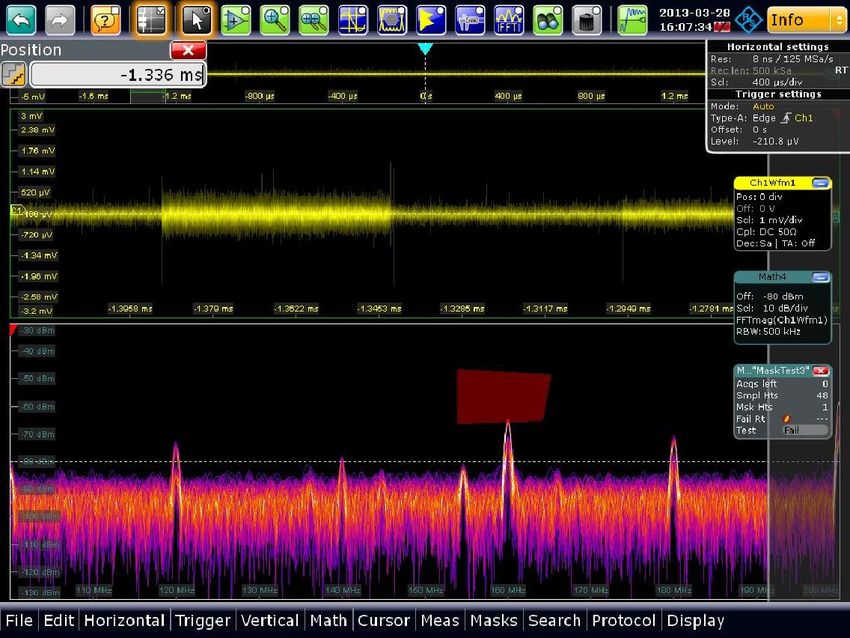
Fig. 4-5: Capturing a sporadically occurring spectral line: The mask violation halts acquisition to
allow detailed investigation of the signal.
Increase in maximum record length for FFT display to allow measurement of
very long signal sequences
Sometimes it is necessary to increase the maximum record length for the FFT
calculation. This involves setting the "Record length limit" parameter in the horizontal
setup dialog. By default, it is set to 1 MS (Msample) in order to ensure a fast response
® ®
by the FFT function. Using an R&S RTO four-channel instrument with the R&S RTO-
B101 memory expansion, this parameter can be increased up to a value of 25 MS.
1.1e Rohde & Schwarz EMI Debugging with the R&S®RTO and R&S®RTE Oscilloscopes 29Practical Aspects of EMI Debugging with the R&S®RTO Digital Oscilloscope
Fig. 4-6: Setting the maximum record length.
Limitations when using oscilloscopes for EMI debugging
An oscilloscope with a powerful spectral analysis function is a very useful tool for
solving EMI problems. However, an oscilloscope is no substitute for a test receiver. As
such, it is important to keep in mind the limitations that apply when using an
oscilloscope. This includes:
ı Limited dynamic range
Oscilloscopes typically use A/D converters with significantly less resolution than
test receivers and thus have much less dynamic range. In EMI debugging, this is
usually not a limiting factor since in most cases we are interested only in the
maximum emissions.
ı No preselection
Oscilloscopes do not have preselection. For this reason, strong interferers outside
of the spectral range of interest can lead to unwanted intermodulation products in
the frequency band of interest. During EMI debugging using near-field probes, this
is typically not a limiting factor since the near-field probe's spatial selectivity
ensures that RF emissions are measured only in the immediate vicinity of the
location where the probe is placed.
ı No standard-compliant detectors
®
Although the R&S RTO has average value and RMS detectors, they do not offer
CISPR standard-compliant functionality. However, a CISPR-compliant detector is
generally not required for EMI debugging applications.
4.2.3 Tips & Tricks for EMI Debugging with the R&S®RTO
ı Avoid overloading
In order to obtain correct results with the spectral analysis function, it is important
to make sure the oscilloscope is not overloaded. Overloading occurs when the
measured signal can no longer be fully displayed on the screen. This is very
important when working with a near-field probe since large amplitude differences
are encountered that can easily cause overloading. Besides false spectral
1.1e Rohde & Schwarz EMI Debugging with the R&S®RTO and R&S®RTE Oscilloscopes 30You can also read