Euclid preparation: XIII. Forecasts for galaxy morphology with
←
→
Page content transcription
If your browser does not render page correctly, please read the page content below
Astronomy & Astrophysics manuscript no. main                                                                                        ©ESO 2022
                                               January 11, 2022

                                                Euclid preparation: XIII. Forecasts for galaxy morphology with the
                                                          Euclid Survey using deep generative models
                                               Euclid Collaboration: H. Bretonnière1,2? , M. Huertas-Company2,3,4,5 , A. Boucaud2 , F. Lanusse6 , E. Jullo7 , E. Merlin8 ,
                                                    D. Tuccillo9 , M. Castellano8 , J. Brinchmann10,11 , C.J. Conselice12 , H. Dole1 , R. Cabanac13 , H.M. Courtois14 ,
                                                 F.J. Castander15,16 , P. A. Duc17 , P. Fosalba15,16 , D. Guinet14 , S. Kruk18 , U. Kuchner19 , S. Serrano15,16 , E. Soubrie1 ,
                                                      A. Tramacere20 , L. Wang21,22 , A. Amara23 , N. Auricchio24 , R. Bender25,26 , C. Bodendorf26 , D. Bonino27 ,
                                                E. Branchini28,29 , S. Brau-Nogue13 , M. Brescia30 , V. Capobianco27 , C. Carbone31 , J. Carretero32 , S. Cavuoti30,33,34 ,
                                                      A. Cimatti35,36 , R. Cledassou37,38 , G. Congedo39 , L. Conversi40,41 , Y. Copin42 , L. Corcione27 , A. Costille7 ,
                                               M. Cropper43 , A. Da Silva44,45 , H. Degaudenzi20 , M. Douspis1 , F. Dubath20 , C.A.J. Duncan46 , X. Dupac41 , S. Dusini47 ,
arXiv:2105.12149v3 [astro-ph.GA] 10 Jan 2022

                                                      S. Farrens6 , S. Ferriol42 , M. Frailis48 , E. Franceschi24 , M. Fumana31 , B. Garilli31 , W. Gillard49 , B. Gillis39 ,
                                                      C. Giocoli50,51 , A. Grazian52 , F. Grupp25,26 , S.V.H. Haugan53 , W. Holmes54 , F. Hormuth55,56 , P. Hudelot57 ,
                                                 K. Jahnke56 , S. Kermiche49 , A. Kiessling54 , M. Kilbinger6 , T. Kitching43 , R. Kohley41 , M. Kümmel25 , M. Kunz58 ,
                                                H. Kurki-Suonio59 , S. Ligori27 , P.B. Lilje53 , I. Lloro60 , E. Maiorano24 , O. Mansutti48 , O. Marggraf61 , K. Markovic54 ,
                                                        F. Marulli24,35,62 , R. Massey63 , S. Maurogordato64 , M. Melchior65 , M. Meneghetti24,62,66 , G. Meylan67 ,
                                                     M. Moresco24,35 , B. Morin6 , L. Moscardini24,35,62 , E. Munari48 , R. Nakajima61 , S.M. Niemi18 , C. Padilla32 ,
                                                 S. Paltani20 , F. Pasian48 , K. Pedersen68 , V. Pettorino6 , S. Pires6 , M. Poncet38 , L. Popa69 , L. Pozzetti24 , F. Raison26 ,
                                                R. Rebolo3,4 , J. Rhodes54 , M. Roncarelli24,35 , E. Rossetti35 , R. Saglia25,70 , P. Schneider61 , A. Secroun49 , G. Seidel56 ,
                                                       C. Sirignano47,71 , G. Sirri62 , L. Stanco47 , J.-L. Starck6 , P. Tallada-Crespí72 , A.N. Taylor39 , I. Tereno44,73 ,
                                                R. Toledo-Moreo74 , F. Torradeflot32,72 , E.A. Valentijn22 , L. Valenziano24,62 , Y. Wang75 , N. Welikala39 , J. Weller25,26 ,
                                               G. Zamorani24 , J. Zoubian49 , M. Baldi24,62,76 , S. Bardelli24 , S. Camera27,77,78 , R. Farinelli79 , E. Medinaceli24 , S. Mei2 ,
                                                       G. Polenta80 , E. Romelli48 , M. Tenti62 , T. Vassallo25 , A. Zacchei48 , E. Zucca24 , C. Baccigalupi48,81,82,83 ,
                                                   A. Balaguera-Antolínez3,4 , A. Biviano48,81 , S. Borgani48,81,83,84 , E. Bozzo20 , C. Burigana85,86,87 , A. Cappi24,64 ,
                                                  C.S. Carvalho73 , S. Casas6 , G. Castignani35 , C. Colodro-Conde4 , J. Coupon20 , S. de la Torre7 , M. Fabricius25,26 ,
                                                  M. Farina88 , P.G. Ferreira46 , P. Flose-Reimberg57 , S. Fotopoulou89 , S. Galeotta48 , K. Ganga2 , J. Garcia-Bellido90 ,
                                                    E. Gaztanaga15,16 , G. Gozaliasl91,92 , I.M. Hook93 , B. Joachimi94 , V. Kansal6 , A. Kashlinsky95 , E. Keihanen92 ,
                                                 C.C. Kirkpatrick59 , V. Lindholm92,96 , G. Mainetti97 , D. Maino31,98,99 , R. Maoli8,100 , M. Martinelli90 , N. Martinet7 ,
                                               H.J. McCracken101 , R.B. Metcalf24,35 , G. Morgante24 , N. Morisset20 , J. Nightingale102 , A. Nucita103,104 , L. Patrizii62 ,
                                               D. Potter105 , A. Renzi47,71 , G. Riccio30 , A.G. Sánchez26 , D. Sapone106 , M. Schirmer56 , M. Schultheis64 , V. Scottez57 ,
                                               E. Sefusatti48,81,83 , R. Teyssier105 , I. Tutusaus15,16 , J. Valiviita96,107 , M. Viel48,81,82,83 , L. Whittaker12,94 , J.H. Knapen3,4
                                                                                                 (Affiliations can be found after the references)

                                                                                                                  ABSTRACT

                                               We present a machine learning framework to simulate realistic galaxies for the Euclid Survey, producing more complex and realistic galaxies
                                               than the analytical simulations currently used in Euclid. The proposed method combines a control on galaxy shape parameters offered by analytic
                                               models with realistic surface brightness distributions learned from real Hubble Space Telescope observations by deep generative models. We
                                               simulate a galaxy field of 0.4 deg2 as it will be seen by the Euclid visible imager VIS, and we show that galaxy structural parameters are recovered
                                               to an accuracy similar to that for pure analytic Sérsic profiles. Based on these simulations, we estimate that the Euclid Wide Survey (EWS)
                                               will be able to resolve the internal morphological structure of galaxies down to a surface brightness of 22.5 mag arcsec−2 , and the Euclid Deep
                                               Survey (EDS) down to 24.9 mag arcsec−2 . This corresponds to approximately 250 million galaxies at the end of the mission and a 50 % complete
                                               sample for stellar masses above 1010.6 M (resp. 109.6 M ) at a redshift z ∼ 0.5 for the EWS (resp. EDS). The approach presented in this work
                                               can contribute to improving the preparation of future high-precision cosmological imaging surveys by allowing simulations to incorporate more
                                               realistic galaxies.
                                               Key words. Galaxies: structure – Galaxies: evolution – Cosmology: observations

                                                                                                                          1. Introduction

                                                                                                                          The Euclid Survey (Laureijs et al. 2011) will observe
                                                                                                                          15 000 deg2 (35 % of the visible sky) over six years, both in
                                                ?
                                                    e-mail: hubert.bretonniere@universite-paris-saclay.fr                 the near-infrared and in the optical at a spatial resolution ap-
                                                                                                                                                                     Article number, page 1 of 23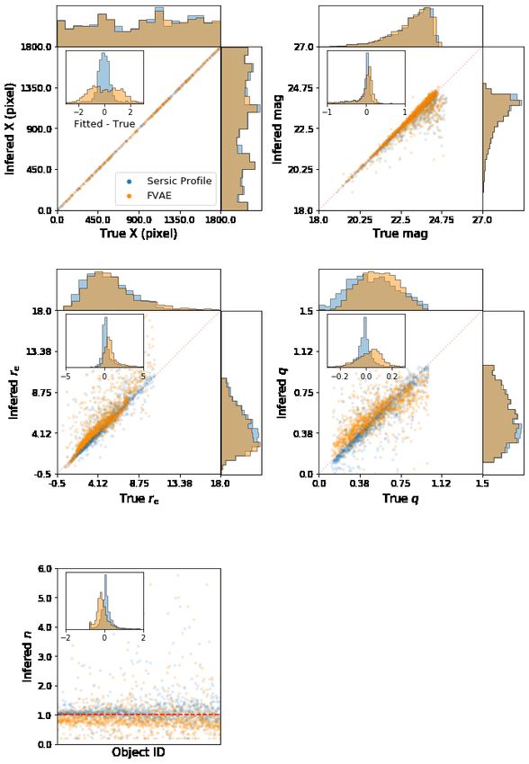
A&A proofs: manuscript no. main

proaching that of the Hubble Space Telescope (HST). With                 morphological limits. We discuss the results of the paper in Sect.
a field of view of 0.53 deg2 , compared to that of the HST               6, and conclude in Sect. 7.
(0.003 deg2 ), it will probe the sky at a rate around 175 times
faster. It will therefore only take around five hours to observe
an area equivalent to the COSMOS field (Scoville et al. 2007),           2. Data
which is still the largest contiguous area ever observed by HST
and needed around 40 days of observations. In addition to the            We use two data sets for this work: the Euclid Flagship galaxy
EWS at an expected nominal depth of 24.5 mag at 10 σ for ex-             catalogue (Castander et al. in prep.), hereafter the Euclid Flag-
tended sources in the visible (Cropper et al. 2016), Euclid will         ship catalogue, and the COSMOS survey (Scoville et al. 2007).
also observe 40 deg2 about two magnitudes deeper (EDS). The              We use the first to simulate best the expected Euclid data as the
limiting surface brightness for the EWS in the visible will be           goal of the paper is to forecast Euclid capacities. The second is
29.8 mag arcsec−2 . We refer the reader to Scaramella et al. (in         used to train our deep learning model so that we lean how to
prep.) for precise information about the Euclid surveys and their        simulate realistic galaxies.
depths.
     Euclid will produce an unprecedented amount of high spa-            2.1. Target set: Euclid Flagship catalogue
tial resolution images that will have a lasting legacy value in a
variety of scientific areas, including cosmology and galaxy for-         To quantify the performance of our model in Euclid-like condi-
mation. In order to ensure that the scientific objectives are met,       tions and establish morphological forecasts for the mission, we
realistic simulations are needed for testing and calibrating al-         used the Euclid Flagship catalogue. We accessed the catalogue
gorithms. A standard approach to simulating galaxy images is             through CosmoHub, a platform that allows the management and
through analytic Sérsic models (Sérsic 1963). It is well known           exploration of very large catalogues, best described in Tallada
that galaxies can be modelled, to a first approximation, with two        et al. (2020) and Carretero et al. (2017).
Sérsic functions, one for the bulge component and the other for              The Flagship catalogue was built using a semi-empirical halo
the disk. Sérsic models have the advantage of being fully de-            occupation distribution (HOD) model and was intended to re-
scribed by three parameters: the Sérsic index, which controls the        produce the global photometric and morphological properties of
steepness of the profile; the effective radius, which measures a         galaxies as well as the clustering. We refer the reader to Merson
characteristic size for the galaxy; and the axis ratio, which re-        et al. (2013) for more details. In order to produce a catalogue
flects the overall shape of the galaxy. Many previous investiga-         close to the real Universe, the morphological parameters, which
tions have shown that Sérsic models reproduce fairly well the            is what we mainly use in this work, are calibrated on the CAN-
average surface brightness distribution of galaxies (e.g. Peng           DELS survey (Dimauro et al. 2018) and 3D model fitting on
et al. 2002). However, because of their simplicity, they are not         the GOODS fields (Giavalisco et al. 2004) by Welikala et al. (in
well suited to describe complex galactic structure such as spiral        prep.). Details about the catalogue production will be presented
arms, bars, clumps, or more generally asymmetric features. This          in Castander et al. (in prep.). Each simulated galaxy in the cata-
is important for the Euclid mission, however, since the spatial          logue is made of two components, a bulge and a disk. The bulge
resolution of the visible detector will permit a significant num-        component is modelled as a Sérsic profile with an index varying
ber of galaxies to be resolved. Complex galaxy morphologies              from n = 0.3 to n = 6. The disk component is rendered using an
can have an impact in the core science of the mission since they         exponential profile (n = 1). The version of the Euclid Flagship
can affect the measurement of shear for weak lensing analysis.           catalogue used in this work contains 710 million galaxies dis-
They are also central to a variety of scientific cases in the field of   tributed over 1200 deg2 , from which we took a random subsam-
galaxy formation. The Euclid data will be particularly important         ple of 44 million galaxies. The distributions of the main morpho-
to constrain the processes that shape the structures of galaxies         logical parameters used in this work are presented in Fig. 1: the
and quench star formation, and will allow us to study the rela-          half-light radius re , the axis ratio q, and the Sérsic index n. We
tions between detailed morphology, environment, active galactic          also show the apparent magnitudes of the galaxies as measured
nuclei activity, and stellar mass, among others (e.g. Lotz et al.        by VIS, which is the visible imager of Euclid (Cropper et al. in
2008; van der Wel et al. 2014; Huertas-Company et al. 2013;              prep.), as well as the redshift and the stellar mass distributions,
Chen et al. 2020; Kocevski et al. 2012; Ferreira et al. 2020; Con-       which we use in Sect. 5 to perform our forecasts. Finally, we
selice 2014). Therefore, in order to quantify the possible effects       show the bulge-to-disk component flux fraction (hereafter bulge
of resolved structures on the image processing pipeline algo-            fraction).
rithms and to best prepare the scientific analysis of the data, it           We note here that the Euclid Flagship catalogue is a pure tab-
is important to produce simulations that include realistic galaxy        ular catalogue. The procedure currently used within the Euclid
morphologies beyond Sérsic models.                                       Consortium to generate the galaxies is described in Sect. 4.1.1,
     In this work we investigate a novel approach based on gener-        when we compare our galaxies to the current analytic ones. Our
ative models to simulate galaxies for the Euclid Survey. We first        work in this study is to use this catalogue of double Sérsic profile
show that our method can generate realistic Euclid galaxy fields         parameters to generate the 2D images of the internally structured
with a level of control of the global shapes that is similar to that     galaxies.
of analytic profiles, but with the addition of complex morpholo-
gies. We then use the generated images to forecast the number            2.2. Training set: COSMOS
of galaxies for which Euclid will resolve the internal structure.
     The paper proceeds as follows. In Sect. 2 we introduce the          The training set is based on the COSMOS survey. COSMOS is
data sets used to analyse Euclid morphological capacities and for        a survey of a 2 deg2 area with the Hubble Space Telescope Ad-
training our models. In Sect. 3 we describe the deep generative          vanced Camera for Surveys (ACS) Wide Field Channel using
model used in this work and its training procedure. In Sect. 4           the F814W filter. The final drizzle pixel scale is of 000. 03 pixel−1
we present our results for the generation of realistic galaxies.         and the limiting point source depth at 5 σ is 27.2 mag. The cen-
In Sect. 5 we use the simulated galaxies to forecast the Euclid          tral wavelength of the F814W filter roughly corresponds to that
Article number, page 2 of 23
H.Bretonnière, M.Huertas-Company, A.Boucaud: Euclid Prep. XIII. Galaxy morphology with deep generative models

of the VIS filter (550 − 900 nm) and the spatial resolution and          Since the pixel size is increased, we can crop up to a factor
depth are better than those expected from the Euclid Survey.             of three without losing spatial covering. However, because our
Therefore, the data set is well suited and is expected to be close       model is more efficient with images that have a number of pixels
enough to the Euclid data, allowing us to generate mock Euclid           which is a power of two (for parity reasons between the compres-
fields without being affected by the dependence of morphology            sion and decompression steps of our deep learning network), we
on wavelength and without introducing undesired effects owing            crop our image by only a factor of two, resulting in images of
to extrapolations.                                                       64 × 64 pixel. The purpose of this cropping is to accelerate the
    Our selected sample is based on the catalogue by Mandel-             training. We finally rotate the stamps so that the galaxy semi-
baum et al. (2012), which has a magnitude limit of 25.2 and              major axis is aligned with the x-axis of the image. With this con-
contains 87 630 objects. The catalogue provides, for each galaxy,        figuration we ensure that our model will learn to produce only
the best-fit parameters of a one-component and a two-component           ‘horizontal’ galaxies and therefore position angles can be man-
Sérsic fit by Leauthaud et al. (2007), updated in 2009. In this          ually added in post-processing. This has the additional advan-
work, we use only the one-component fitting information. In              tage of reducing the complexity and hence allowing the neural
Fig. 1 we show the distribution of the COSMOS morphologi-                network to focus the attention on the more important physical
cal parameters of galaxies compared to those in the Euclid Flag-         properties of the object. Figure 2 illustrates these pre-processing
ship catalogue. Although the distributions are similar, there are        steps used for the training of our model, and the final galaxy as it
some noticeable differences which might cause a problem. The             would be seen by VIS. Because galaxies produced by our model
most obvious one is the magnitude. Since COSMOS is magni-                will be noise-free and not convolved by the PSF, we do not need
tude limited, the sample does not contain as many faint galaxies         to change the noise level and the PSF for the training. Thus, the
as the simulation. The half-light radii of the Euclid Flagship cat-      inputs of our model have the noise characteristics and the PSF of
alogue bulge component also extend to smaller values than those          the HST images. These two transformations, to go from HST to
in the observations. They are also generally rounder than the ob-        Euclid data will be added a posteriori. More information about
served ones, but the values of axis-ratios span a similar range.         those transformations are described Sects. 4.1.1 and 4.2.2.
The Sérsic index distributions are also different because, as ex-            We use the COSMOS catalogue and images only for the
plained previously, the Euclid Flagship disk component always            training of our model. To test the performance of our model
has a Sérsic index of 1. In addition, in the COSMOS catalogue            (Sect. 4) and the forecasts (Sect. 5), we only use the Euclid Flag-
the Sérsic indices of the bulge component are clipped at n = 6           ship catalogue described in the previous section.
to be compatible with GalSim , which creates a noticeable spike
at the edge of the distribution. The mass fraction and redshift
is derived by Laigle et al. (2016). As we show in the follow-            3. Euclid emulator with generative models
ing sections, these differences, although present, do not have a
significant effect on our methodology. The most important de-            In this section we describe the methodology for emulating Euclid
sirable property is that simulated galaxies cover a similar range        galaxies using the COSMOS sample described in the previous
to observations. That way, the neural network used in our model          section.
is not compelled to extrapolate. This is essentially the case in             The generation of synthetic data (images, language, videos)
the distributions shown in Fig. 1, except for very small bulge           has significantly improved in recent years thanks to new deep
components and for very faint galaxies, both of which are not            learning-based generative models. Generative models are a type
expected to present significant features. We address these points        of unsupervised machine learning algorithms that are trained to
in the following sections.                                               generate unseen data. There are several architectures; variational
    In addition to the catalogue, the authors also provide 128 ×         autoencoders (VAE: Kingma & Welling 2013), generative adver-
128 pixel stamps centred on each galaxy where neighbouring               sarial networks (GANs: Goodfellow et al. 2014; Arjovsky et al.
galaxies have been removed. This is important for training our           2017), and autoregressive models (van den Oord et al. 2016) are
model on a unique galaxy per stamp. Therefore, the impact of             the main ones. They all learn a probability distribution function
galaxy blending in the morphology forecasts will not be studied          of the pixel distribution, which can be sampled to generate new
in this work. In addition, the size of the stamps inherently limits      data. Generative models have already been used in astrophysics
the size of galaxies that we will be able to generate. The radius of     for a variety of different purposes. For example, with VAEs ra-
the stamp being 64 pixels, every galaxy with a half-light radius         dio galaxies can be simulated (Bastien et al. 2021) or images
larger than ∼ 200 will be cut by the limits of the stamp. For this       of overlapping galaxies can be reconstructed separately (Arcelin
reason, in this work we are limited to, and thus only consider,          et al. 2021). Using GANs, Yi et al. (2020) have simulated miss-
galaxies smaller than 200 . Nevertheless, galaxies with a radius         ing data from the cosmological microwave background, while
bigger than 200 represent only 0.6 % of the Euclid Flagship cata-        Villaescusa-Navarro et al. (2020) have simulated gas density
logue, and thus have no major impact on our results.                     maps. Storey-Fisher et al. (2020) and Margalef-Bentabol et al.
    The COSMOS images are pre-processed before they are                  (2020) have used GANs to detect outliers in imaging surveys.
used for training, as illustrated in Fig. 2. We first degrade the        Autoregressive flows can be used to compare simulations and
spatial sampling from 000. 03 pixel−1 to 000. 1 pixel−1 , which corre-   observations (e.g. Zanisi et al. 2021).
sponds to the pixel scale of VIS, and then pad the image with                In this work we use a VAE. Variational autoencoders esti-
the appropriate noise. We use the GalSim (Rowe et al. 2015)              mate an explicit latent space, which is an important advantage for
method described in Sect. 5 of Mandelbaum et al. (2012). Since           simulating galaxies with known parameters. The compression–
the pixel scale increases, the final stamp needs to be padded with       decompression architecture inherent to the VAEs along with the
noise to keep the size of 128 × 128 pixel. The method does this          Kullback–Leibler term in the loss (see Sect. 3.1.1 Eq. 3) force
automatically by adding a noise realisation with the same char-          the latent representation to be meaningful and regular. In addi-
acteristics as in the original stamps, which also takes into ac-         tion, VAEs are known to be more stable during training, and less
count the different correlations in the original noise. Doing so,        subject to mode collapse (lack of diversity in the generation) than
the resulting images are still at the size of the COSMOS stamps.         GANs.
                                                                                                                 Article number, page 3 of 23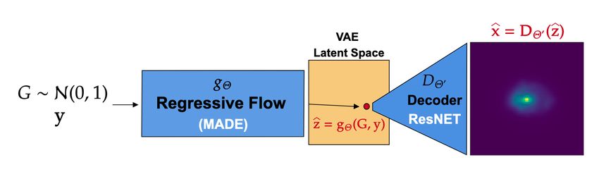
A&A proofs: manuscript no. main

                                                                      Fig. 2: Illustration of our pre-processing pipeline on a random
                                                                      COSMOS image, and the difference between HST and Euclid.
                                                                      The original image (leftmost) is rotated to be aligned with the
                                                                      x-axis of the stamp in the second image from the left, then re-
                                                                      scaled to the VIS resolution and cropped (third image from the
                                                                      left). This is the data used to train our model. In the rightmost
                                                                      image the galaxy was deconvolved by the HST PSF and re-
                                                                      convolved with the Euclid PSF. This final step is shown for il-
                                                                      lustrative purposes, but is not carried out in the pre-processing
                                                                      of the training sample.

                                                                      keeping a control on the shape parameters, such as axis ratios,
                                                                      effective radii, and fluxes. To this end, our model is made of
                                                                      two distinct parts: a variational autoencoder (Kingma & Welling
                                                                      2013), which learns how to simulate real galaxies from obser-
                                                                      vations, and a normalising flow (Jimenez Rezende & Mohamed
                                                                      2015) in charge of mapping catalogue parameters to the VAE
                                                                      latent space. Both parts are merged together after training, re-
                                                                      sulting in an architecture called a flow variational autoencoder
                                                                      (FVAE). We describe in the following the global properties of
                                                                      these two models.

                                                                      3.1.1. Galaxy generation with a variational autoencoder
                                                                      A VAE is a deep generative model which is trained to generate
                                                                      new data (galaxies) by learning a probability distribution from
                                                                      the training data. To this end, the VAE first compresses the input
                                                                      image x into a low-dimensional space, also called latent space,
                                                                      which contains a compact and meaningful representation of the
                                                                      input data. Similar objects are compressed into neighbouring
                                                                      vectors. This is achieved with a convolutional neural network
                                                                      called the encoder, which can be represented as a non-linear
                                                                      function EΘ , Θ being its trainable parameters. While a classi-
                                                                      cal autoencoder compresses the input image only into a vector
                                                                      z, a VAE replaces that low-dimensional vector with a probabil-
                                                                      ity distribution function (PDF) pΘ (z | x). In our case, pΘ (z | x) is
Fig. 1: Distributions of the main structural parameters in the data   set to be a multivariate Gaussian distribution. This is equivalent
sets used in this work, along with the redshift and the stellar       to choosing the prior for the distribution of points in the latent
mass used for our forecasts. We also show the bulge to disk flux      space to be Gaussian. Similar galaxies will be encoded into sim-
fraction (bulge fraction) for the Flagship. The y axis is the nor-    ilar regions of the distribution. Having a distribution instead of a
malised density counts such that the area over the curve is equal     point estimate makes the latent space continuous, allowing one
to one. For the magnitude, the COSMOS histogram shows the             to sample new regions from it and to produce new galaxies aris-
F814W magnitude and the Flagship one corresponds to the Eu-           ing from the same probability density function as the data.
clid VIS magnitude. The range of the training set (COSMOS)                 A sample z is then drawn from the distribution pΘ . This con-
covers most of the Euclid data.                                       stitutes the input of a second convolutional neural network called
                                                                      the decoder DΘ0 , which typically has an architecture symmetric
                                                                      to that of the encoder. The decoder decompresses the latent rep-
3.1. Model                                                            resentation z using transposed convolutions to produce a new im-
                                                                      age x̂, DΘ0 (z) = x̂. The output of the decoder can be seen as the
Our model for generating galaxies is based on the work by             probability that the input data x effectively come from the latent
Lanusse et al. (2020) (hereafter L2020) who describe in detail        space vector z (i.e. DΘ0 (z) = pΘ0 (x | z)). During training, the goal
the architecture and specifics of the training procedure. We also     is to reconstruct x with the best possible accuracy (i.e. x̂ = x) en-
illustrate the architecture of the two components of our model in     suring that the distribution encoded within the latent space is a
Figs. B.1 and B.2.                                                    good representation of the data. The amount of information loss
    The goal of our work is to simulate and test galaxies with        in the compression–decompression is the first term of the neu-
more realistic shapes than the classical analytic profiles while      ral network loss function L, which is used to adapt Θ and Θ0
Article number, page 4 of 23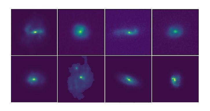
H.Bretonnière, M.Huertas-Company, A.Boucaud: Euclid Prep. XIII. Galaxy morphology with deep generative models

through a gradient descent minimisation. From a statistical point            If the mapping is well learnt, when we sample a vector zflow
of view, this accuracy is defined as the negative log-likelihood of      from the flow latent space distribution q and pass it through gΘ
x given z, which can be written using the expectation value:             along with a vector of physical parameter y, it will output a vec-
                                                                         tor ẑ in the VAE latent space
L = − E z∼pΘ (z | x) log pΘ0 (x | z) .

                                                                (1)
                                                                         ẑ = gΘ (zflow , y) ,                                             (5)
    In practice, we can simply see the reconstruction accuracy as
the mean square error between the reconstructed image and the            such that ẑ is very similar to the vector z, which would have been
input:                                                                   encoded by the VAE’s encoder from a galaxy x with physical
                                                                         parameters y

L = kx − x̂k2 .                                                   (2)    ẑ ≈ EΘ (x y ) .                                                  (6)
                                                                         With this mapping, we now know where to sample into the VAE
In addition, in order to regularise pΘ , a second term is added to
                                                                         latent space in order to decode a galaxy with precise physical
penalise the encoder when it produces distributions too far from
                                                                         parameters: to simulate a galaxy, we need to map zflow and y
a normal Gaussian distribution N(0, 1). This difference between
                                                                         to the VAE latent space, and then decode the vector with the
pΘ (z | x) and N(0, 1) is estimated using the Kullback–Leibler di-
                                                                         decoder to produce an image of a galaxy that has the physical
vergence (Kullback & Leibler 1951):
                                                                         properties given by y.
KL = E[log pΘ (z | x) − log N(0, 1)] .                            (3)         In practice, the training procedure is done the other way
                                                                         around: we learn how to map a vector z = EΘ (x) into a vector
The final loss function for the VAE reads                                zflow of the flow latent space. Because gΘ is a bijector, learning
                                                                         the mapping from the flow latent space to the VAE latent space
                                                                         or the other way around is the same task, but doing it in this di-
L = −E z∼pΘ0 (z | x) log pΘ0 (x | z) +

                                                                         rection is much easier because of the loss. The loss we use is
     β E[log pΘ (z | x) − log N(0, 1)] ,                          (4)    the negative log likelihood of z under the distribution of the flow
                                                                         latent space q
where β allows us to vary the importance of the terms during
                                                                         Lflow = E z∼p − log p(z)

training.                                                                                 h                                    i
    Lanusse et al. also introduce two additional features in order              = E z∼p − log q g−1 (z) + log det Jg−1 (z) ,              (7)
to produce images deconvolved by the PSF and without noise. To                              h                                      i
learn noise-free galaxies, a different version of the log-likelihood            = E zflow ∼q − log q (zflow ) + log det Jg (zflow ) ,     (8)
for the reconstruction term of the loss function is used. Instead
of applying it directly to the pixels, it is done in Fourier space       where det Jg , the determinant Jacobian of g, comes from the
in order to weight the reconstruction error less on the high fre-        transformation between the two distributions.
quencies (noisy regions). The Fourier transform of the input and             Choosing a standard Gaussian distribution for q, we ensure
of the output is computed, and divided by the power spectrum             that this loss is tractable (i.e. easy to compute). By construction,
of the noise. By dividing the Fourier transform of the image by          the Jacobian of g is also easy to compute (Kobyzev et al. 2019).
the power spectrum of the noise, a smaller weight is given to the        Thus, during training, every galaxy x is encoded by the previ-
pixels with a high frequency. It ensures that the decoder learns         ously trained encoder E into a vector z drawn from the encoded
that producing images without noise is not an error. In order to         distribution pΘ (z | x). This vector z is transformed by the flow’s
produce deconvolved images, the last convolutional layer of the          bijector g−1
                                                                                    Θ into a vector zflow conditioned by the physical pa-
decoder is not trainable and is set to be equal to the PSF. That         rameters of the galaxy y
way, the model produces an image that looks like the input image         zflow = g−1
                                                                                  Θ (z, y) ,                                               (9)
before being convolved by the PSF in the second last layer.
                                                                         which is used to compute the loss and optimise the weights of g.
                                                                             To implement the flow, we use the probabilistic library of
3.1.2. Sample of the shape parameters with the regressive
                                                                         TensorFlow, TensorFlow probability. With this library it
       flow
                                                                         becomes straightforward to implement the bijector g, with a
The VAE described in the previous subsection can generate real-          chain of masked autoregressive layers, described in Germain
istic galaxies by sampling from the encoded latent space. How-           et al. (2015). The transformations of the distribution made by
ever, it cannot do so for a given size or ellipticity because it lacks   the successive layers (shifts of the mean and stretch of the dis-
the information about the mapping between the structural param-          persion) are conditioned to the physical parameters of the flow’s
eter space of the galaxy and the latent space.                           input. Then, thanks to the Distribution object of the library,
     To learn that mapping, L2020 propose a conditional nor-             with only one command it is possible to sample the transformed
malising flow, based on autoregressive algorithms (MAF: Papa-            distribution (e.g. to get zflow ), but also to take the log likelihood
makarios et al. 2017, MADE: Germain et al. 2015). A normalis-            for the computation of the loss.
ing flow is a bijector gΘ , which transforms a distribution q into
another distribution p with an invertible transformation g. We           3.1.3. Final model
use it here to learn the mapping between a latent space with a
fixed distribution q, referred to as the flow latent space, and the      The final model (schematic representation in Fig. 3) combines
distribution p inside the VAE latent space. This mapping can be          the decoder part of the VAE with the regressive flow described
made conditional to some input parameters y such as galaxy size          in the previous subsection. Therefore, the input of the final model
or ellipticity. In other words, gΘ is a function of both the latent      is a galaxy catalogue. The flow samples a Gaussian noise vector,
space vector z and the physical parameters of the galaxy y.              which is concatenated with the catalogue parameters to produce
                                                                                                                  Article number, page 5 of 23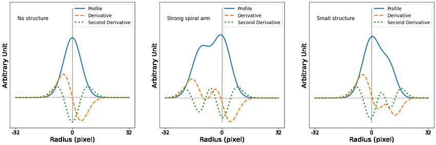
A&A proofs: manuscript no. main

                                                                      4. Emulation of VIS images
                                                                      In this section we analyse the properties of simulated galaxies
                                                                      and assess the accuracy of the emulation. Our emulator is ex-
                                                                      pected to fulfil two main goals: realistic galaxies and a control
                                                                      on the global shape parameters.

                                                                      4.1. Simulation of composite galaxies
Fig. 3: Schematic representation of the FVAE architecture used
to simulate a galaxy with structural parameters y. A random           4.1.1. Simulations with pure Sérsic profiles
noise G is passed through a regressive flow conditioned to the
input galaxy parameters y. The flow outputs a latent space vec-       The Euclid Consortium currently creates analytic galaxies with
tor ẑ, which is decoded by the VAE in order to produce a galaxy      the GalSim software (Rowe et al. 2015). Each galaxy is created
corresponding to the input shape parameters.                          as the sum of two components, the bulge and the disk. The disk
                                                                      component is created with an exponential profile (Sérsic profile
                                                                      with n = 1). The bulge component is a 3D Sérsic profile, which is
                                                                      projected to produce the expected ellipticity. The two profiles are
a vector in the latent space. The vector is then decoded by the       created with the expected bulge-to-disk flux fraction, and then
generator of the VAE, producing the image of a new galaxy with        summed pixel-wise. The flux is then rescaled to match the total
the corresponding input parameters from the catalogue. The use        galaxy magnitude. The image is finally convolved with the VIS
of a continuous distribution enables the generation of new galax-     PSF, which has a full width at half maximum (FWHM) of 000. 17
ies that resemble real ones, but have never been observed before.     at 800 nm (Laureijs 2017). This PSF takes into account all the
                                                                      optical and instrumental effects, and thus goes beyond a simple
                                                                      Gaussian. It is the result of the detailed analysis of the VIS in-
                                                                      strument performed by the Euclid Consortium. If necessary, we
3.2. Training procedure                                               also rotate the galaxy to its corresponding position angle in the
                                                                      sky. At this stage, the galaxies are noise-free. The method used
The main goal of this work is to produce Euclid-like realistic        to add noise is explained in Sect. 4.2.2.
galaxies. We use pre-processed COSMOS galaxies (described in
Sect. 2) to train the VAE. We train it for 250 000 steps, which
means 3900 epochs (one epoch is when the whole training set           4.1.2. Simulations with the FVAE
has been seen by the network) with a batch size of 64 (the            Once trained, our model takes as input the three shape parame-
batch size is the number of images with which we perform each         ters of each component of the galaxy from the Euclid Flagship
gradient descent). The latent space has a dimensionality of 32.       catalogue (half-light radius re , Sérsic index n, and axis ratio q)
The learning rate has a first phase where it linearly increases,      and generates a galaxy with the expected structure and realistic
followed by a square root decay. We use a warm-up phase of            morphology. As explained above, galaxies in the Flagship cata-
30 epochs where we train only the generative part (β = 0 in           logue are described by two components, a bulge and a disk. To
Eq. 4), and then linearly increase it to have the same weight         simulate exactly the same field and compare to the current Eu-
between the generative term of the loss function and the KL           clid simulations, we also need to produce the two components
(β = 1). Training and validation losses converge long before the      separately. This way, we can reproduce the same method as the
end of training. However, even after the convergence, we still see    current Euclid procedure explained in the previous subsection.
a significant improvement in the generated images. The model          Each component (bulge and disk) is simulated separately by our
first learns the global shape of the galaxies and a Gaussian pos-     model, and then added with the appropriate bulge-to-disk flux
terior in the latent space, making the objective function Eq. (4)     ratio. We then use GalSim to scale the flux, to convolve by the
already very low. The learning of more complex structures inside      PSF, and to rotate the galaxy to the appropriate position angle.
the galaxies does not have a great impact on the loss (most of the    Since the flux is calibrated in the post-processing step, we can
galaxies do not present major structures and the pixels belonging     associate faint magnitudes with our emulation even if not prop-
to the structures represent a small fraction of the image), which     erly covered by our training set, as shown in Sect. 2. For the
can explain why we need to train longer than the convergence          other parameters, as the distributions of the bulges and the disks
to learn the complex distribution of the training set. We show in     in the Flagship are covered by the training set, simulating the
the following sections that we chose an appropriate number of         two components separately should not be an issue.
epochs to produce complex galaxies without overfitting. We did
not try to optimise this number of epochs, the balance between
results and training time being sufficient for our study. Neverthe-   4.2. Qualitative inspection
less, the large number of epochs is not unusual, and generative
models such as VAEs usually require a large number of epochs          4.2.1. Individual noise-free galaxy simulation
to converge.                                                          We first qualitatively evaluate our simulations. Figure 4 shows
     In a second step, we tackle the regressive flow. We condition    eight galaxies with large radius, prone to presenting interest-
the model with three parameters: Sérsic index n, half-light radius    ing morphologies. Compared to pure Sérsic profile simulations,
re , and axis ratio q. We trained it for 470 epochs, ensuring that    the generated galaxies are more complex and asymmetric (see
both our training and validation loss had converged. We use a         Fig. A.2 for some examples of pure Sérsic galaxies). We are able
batch size of 128, and the same learning rate strategy as for the     to generate the commonly observed features such as rings, spiral
VAE. By design, the dimensionality of the flow latent space is        arms, irregularities, and clumps with different inclination angles.
the same as that of the VAE (i.e. 32 in this work).                   This visual inspection is a first indication that we are able to gen-
Article number, page 6 of 23
H.Bretonnière, M.Huertas-Company, A.Boucaud: Euclid Prep. XIII. Galaxy morphology with deep generative models

Fig. 4: Example of galaxies simulated by the FVAE presenting
obvious complexity and features. The scale is linear.

erate complex behaviour and mimic surface brightness profiles
or features superior to those of Sérsic profile simulations.
     The second key element of our emulator is the ability to
control the structural parameters. In order to illustrate this, we
show in Figs. 5 and 6 the impact of varying parameters on the
generated galaxies. Figure 5 shows a series of generated galax-
ies with a constant magnitude set to 24, a fixed Sérsic index of
                                                                     Fig. 5: Galaxies simulated by our model from a catalogue with
1.5 and a varying axis-ratio q and half-light radius re . Figure 6
                                                                     increasing axis ratios (q) and effective radius (re ). The magni-
shows a grid of galaxies with fixed re and magnitude but varying
                                                                     tude and the Sérsic index are fixed to 24 and 1, respectively, for
axis-ratio and Sérsic index. We can clearly observe the expected
                                                                     all galaxies. The images are all 64 × 64 pixel, the natural out-
trends. Galaxies become rounder as we move from left to right,
                                                                     put of our model. Each row shows galaxies with constant re , and
and bigger from top to bottom in Fig 5. In Fig. 6 galaxies be-
                                                                     linearly increasing q from 0.1 to 0.95. Each column shows galax-
come more concentrated as the Sérsic index increases from left
                                                                     ies with fixed q, and linearly increasing re from 000. 1 to 100 . The
to right. The images also show several examples presenting non-
                                                                     galaxies are clearly rounder and bigger from left to right and top
trivial symmetric shapes. An important limitation to note is that
                                                                     to bottom.
our model is fixed to produce images of size 64 × 64 pixel. Very
large galaxies might therefore be truncated.
                                                                     shapes and controlling structural parameters. However, in order
4.2.2. Large field simulation                                        for the simulation to be useful to test algorithms, it is required
In addition to individual stamps, we also generate two large         that the control on the structural parameters is comparable to
fields of 0.4 deg2 at the depths of the EWS and the EDS (see a       what is achieved with analytic profiles.
portion of those fields in Fig. 7). We take a subsample of the Eu-
clid Flagship catalogue and generate every galaxy without noise      4.3.1. Surface brightness profiles
and deconvolved by the PSF. We then convolve the stamp by
a unique VIS PSF (no PSF variations are modelled). All the           We compare the radial profiles of generated galaxies with the
stamps are then placed in the large field into their corresponding   profiles of analytic galaxies with the same global properties. Fig-
positions according to the catalogue. We finally add the expected    ure 8 compares and shows the radial profile for three bulge com-
noise level of the EWS and the EDS in two different realisations     ponents, disk components, and the combination of the two com-
of the same field. The background noise (coming mostly from          ponents, simulated with our model and with GalSim . All the
background sources and from the zodiacal light) is simulated by      images are convolved by the VIS PSF but are without noise. We
Gaussian noise with the expected standard deviation for the VIS      show both the profile along the major axis and the azimuthally
camera (Cropper et al. in prep.; Scaramella et al. in prep.; priv.   averaged profile. The former is useful to identify deviations from
comm.). The photon noise is simulated with a Poisson distribu-       a smooth profile, and thus highlights where the irregularities take
tion added to every pixel, considering the cumulative exposure       place. The latter, computed by averaging the luminosity at a
times presented by Laureijs et al. (2011).                           given radius r from the galaxy centre in all directions, allows
    More information will be given about the noise realisations      us to check if the average profile behaves as expected compared
in Merlin et al. (in prep.). We do not simulate any instrumental     to the Sérsic model. Overall, the figure shows the expected be-
effects such as cosmic rays, ghosts, charge transfer inefficiency,   haviour. Some profiles deviate significantly from a Sérsic profile
or read-out noise, considering thus an ideal case of a VIS image     along the major axis. An example for this is the disk component
processing pipeline. In Fig. 7 we show a random region of the        shown in the bottom row of Fig. 8, where we can see a spiral arm
large fields, and highlight some interesting galaxies.               feature that creates variation in the radial light profile. However,
                                                                     the average profiles tend to follow the analytic expectations since
4.3. Quantification of structural properties                         irregularities are averaged out. Therefore, the generated galax-
                                                                     ies seem to present the desired behaviour (i.e. complex surface
This visual assessment of the previous subsection confirms that      brightness distributions), which on average match a Sérsic pro-
our model behaves as expected both in generating complex             file. An additional interesting result seen in Fig. 8 is that the
                                                                                                              Article number, page 7 of 23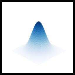
A&A proofs: manuscript no. main
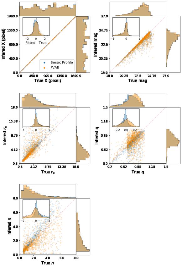
Figures 9 and 10 show the fitting results concerning bulge
and disk components, respectively, for five parameters: half-light
radius re , axis ratio q, Sérsic index n, centroid position X, and to-
tal magnitude. We recall that the goal of this comparison is not
to quantify the absolute accuracy of the fits, but to compare the
relative behaviour of our simulations with a baseline. A future
publication in preparation will quantify in detail the accuracy
of structural parameters in both the EWS and the EDS. Overall,
the structural parameters are recovered with similar dispersion
for the FVAE and the analytic simulation. This is a first quanti-
tative confirmation of the visual inspection of the previous sec-
tions. Our model is able to produce realistic galaxy images while
preserving information on the parametric structure. The global
distributions of the predicted parameters are also very similar,
which confirms that our model has correctly learnt the entire
distribution of the training set, and is thus able to span the en-
tire parameter space of the Euclid Flagship catalogue.
Looking in more detail, the FVAE results present a slightly
larger dispersion in all recovered parameters. This is expected
since the analytic simulations represent a perfect match for the
model that is fitted. This is not the case for the FVAE simula-
tions, which present more complex profiles. We give the statis-
tical details of the fitting distribution errors (median, first, and
Fig. 6: Galaxies simulated by our model from a catalogue with third quartile) in Table 1, corresponding to the distributions in
increasing axis ratios (q) and Sérsic indices (n). The magnitude the insets in each panel of Figs. 9 and 10.
and the effective radius are fixed to 24 and 000. 7, respectively, for The systematic offsets might be more problematic. The fig-
all galaxies. Each row shows galaxies with constant q, and lin- ure shows that the systematic shifts for the bulge components are
early increasing n from 1 to 4. Each column shows galaxies with very similar for the analytic and the FVAE fields which means
fixed n, and linearly increasing q from 0.1 to 0.95. The galaxies that using a FVAE does not introduce any noticeable system-
clearly show a steeper profile and are rounder from left to right atic effects. The only parameter that presents a small bias to-
and top to bottom, respectively. wards larger values is the axis ratio q. This might be because of
a lack of very elongated bulges in the training data set. The disk
components present a slightly higher systematic bias though, as
combination of the two components also behaves very similarly shown in Fig. 10. Indeed, FVAE galaxies tend to be systemat-
when compared to a double-component analytic galaxy (see the ically larger and rounder than their analytical counterparts and
composite galaxy column). show an almost constant offset of 0.15 on the Sérsic index. It
is not obvious whether these offsets are a consequence of the
simulation or whether it is related to the fitting procedure itself.
4.3.2. Surface brightness fitting
A possible explanation for the larger offsets is that disk compo-
We now fit Sérsic models to quantify how accurately the shape nents are generally more extended and with flatter profiles than
parameters are recovered in a statistical sense. For this pur- bulge components, thus they also present more complexity and
pose we use the Galapagos package (Barden et al. 2012; structure. Alternatively, it can also be related to the simulation
Häußler et al. 2013). Galapagos is a high-level wrapper for itself. Our training set is based on a single-component fit with
SExtractor (Bertin & Arnouts 1996) and Galfit (Peng et al. a continuous distribution of the Sérsic index. However, the Sér-
2002) to automatically fit large samples of galaxies. Because sic index of the disk component in the Euclid Flagship catalogue
two-component Sérsic fits are generally less stable than one- is fixed to n = 1. This means that there is only a small number
component fits (e.g. Simard et al. 2011, Bernardi et al. 2014, of examples in the training set with exactly n = 1, which can af-
Dimauro et al. 2018) we decide to produce the two components fect the quality of the generation. Finally, we can see that for the
separately in two distinct realisation of the field. Thus, we have magnitude, the fit of our galaxies also differs very little from the
two different fields, one with only the bulge component and one Sérsic fits, even if the flux is not something that is parametrised
with only the disk component. We then fit each field with the in our model, but re-scaled afterwards with Galsim. This occurs
one-component Sérsic model. This allows us to test the relia- because the recovering of the flux in a large field, with blended
bility of the fits while reducing the degeneracies. Since our ob- galaxies for example, is not completely trivial.
jective is to compare our simulation to an analytic one, a single
Sérsic fit is enough for our purpose.
Using the Euclid Flagship catalogue, we generate with our
model a galaxy field of 0.4 deg2 (i.e. around 2500 galaxies with 5. Forecasts for galaxy morphology with Euclid
magnitude lower than 25), following the same procedure as in
Sect. 4.2.2. We then use the same procedure and subsample to The previous sections have shown that our proposed framework
produce the same field with the pure Sérsic profiles. The two successfully generates galaxies with realistic and resolved struc-
fields are therefore identical in terms of number of galaxies and ture. Our simulations can therefore be used to establish some
positions, and contain galaxies with the same structural proper- forecasts on the number of galaxies for which Euclid will be
ties. able to resolve the internal structure beyond a Sérsic profile.
Article number, page 8 of 23H.Bretonnière, M.Huertas-Company, A.Boucaud: Euclid Prep. XIII. Galaxy morphology with deep generative models
(2)
(3) (4)
(5)
(3)
(4)
(1) (2)
(5)
(1)
(6)
(6)
(2)
(3) (4)
(5)
(3)
(4)
(1) (2)
(5)
(1)
(6)
(6)
Fig. 7: Illustration of a large field simulation produced by our FVAE. The top and bottom panels show the same field simulated at
the depths of the EDS and the EWS, respectively. The stamps show zoomed-in regions where some galaxies present morphological
diversity. In the large field images, we use the IRAF ‘zscale’ that stretches and clips the low and high values to better highlight the
differences between the EWS and the EDS. The stamps are in linear scale, which better emphasises the structures. With the stretching
induced by the zscale, all the structures disappear and only the global shape is still recognisable. Finally, the apparent different level
of background between the stamps and the global image is also due to the different brightness scale (different maximum and
minimum values in each of them).
Article number, page 9 of 23A&A proofs: manuscript no. main
Fig. 8: Examples of three radial profiles of galaxies generated with GalSim and our model. Each group of two columns represents
the different components of the galaxy: bulge, disk, and composite (bulge plus disk) from left to right. Within each group the top
row shows the images by our model (left) and by the Sérsic model (right). The bottom line represents the light radial profiles, along
the major axis (left) and the average profile (right). The orange lines correspond to our model, and blue to the Sérsic profile. The
dashed grey line represents the EWS noise level. Our simulations show more diverse profiles, but the average closely matches the
analytic expectations. The irregularities at very low S/N on the FVAE profiles are a sign that the model does not produce perfectly
noise-free galaxies.
5.1. Identifying galaxies with resolved structure ing its sign only at the centre of the galaxy. If we consider only
a one-sided profile, the derivative never goes to zero (i.e. it has
Our goal is to quantify the fraction of galaxies that present sig- no roots). Its second derivative is also smooth, and has only one
nificant structures that deviate from a pure analytic profile. For root that we call a ‘natural zero’. When the galaxy is strongly
that purpose we have designed a method to distinguish galaxies perturbed, the profile will significantly differ from a pure analyt-
with internal structure from smooth objects. We assume that any ical profile. For a Sérsic profile the light curve decreases from
type of complexity in the galaxy surface brightness distribution, the centre to the edge of the galaxy; instead, for example in a
hereafter called structure, will result in a deviation from an an- galaxy presenting a spiral arm, the major axis profile increases
alytical profile. This is particularly clear in the disk component in the location of the arm. This increase (change of slope) will
shown in Fig. 8. We therefore establish a criterion to characterise cause a sign change in the first derivative, and thus two changes
the smoothness of a galaxy by computing the derivatives of the in sign in the second derivative, as can be seen in the second
semi-major axis profile. For illustration purposes, we show in column of Fig. 11. However, the roots of the first derivative are
Fig. 11 three toy profiles. A pure analytical profile, a profile pre- not always enough to detect a variation from a smooth profile,
senting a strong structure, and a slightly perturbed one. When as illustrated in the third column of the figure; the profile can be
the profile is smooth the first derivative is also smooth, chang- slightly perturbed, with a change of slope in the profile, but this
Article number, page 10 of 23H.Bretonnière, M.Huertas-Company, A.Boucaud: Euclid Prep. XIII. Galaxy morphology with deep generative models
Table 1: Accuracy of fitting results. For each parameter shown in Figs. 9 (bulges) and 10 (disks), we present the first quartile (q1 ),
the median (µ1/2 ), and the third quartile (q3 ) of the fitting error distributions.
Bulges Disks
FVAE
q1 µ1/2 q3 q1 µ1/2 q3
Analytic
−0.36 0.01 0.40 −0.90 −0.01 1.00
X
−0.37 −0.04 0.26 −0.36 −0.05 0.25
−0.33 −0.06 0.03 −0.09 0.04 0.10
mag
−0.25 −0.04 0.03 −0.11 0.01 0.04
−0.23 0.25 1.77 0.27 0.65 1.27
re
−0.04 0.24 1.25 −0.07 0.11 0.55
−0.10 0.00 0.07 −0.04 0.03 0.09
q
−0.10 −0.03 0.00 −0.05 −0.01 0.01
−0.64 −0.06 0.52 −0.29 −0.15 0.04
n
−0.01 0.23 1.26 −0.06 0.06 0.20
does not make the profile rise as in the second column of the fig- We can see that the fraction of galaxies with resolved struc-
ure, but significantly changes the rate of decrease. Thus, the first tures decreases with increasing surface brightness, as expected.
derivative will not change in sign (the profile does not increase), The behaviour of the EWS and the EDS is self-similar, but the
but the second derivative will (the rate of the decrease changes). EDS is shifted towards fainter surface brightness. The differ-
Therefore, we conclude that the presence of a zero on the ence is of the order of 2 magnitudes: less than 10 % of galaxies
second derivative of the light profile (without counting the nat- present detailed structures above 2 σ, beyond a surface bright-
ural zero) is a reasonable indicator of a galaxy with complex ness of 22.5 mag arcsec−2 for the EWS and 24.9 mag arcsec−2
structures. We note that there will be additional zeros at the edge for the EDS. The statistical fluctuations on the curve are similar
of the profile when it becomes flat. However, these roots will because we compute our structure indicator on the same realisa-
be all consecutive, giving us a way to distinguish zeros coming tions of galaxies with only the S/N changing.
from a structure from ones coming from the end of the profile.
We also provide the total number of galaxies per bin in the
Thus, we can consider a galaxy being structured if its second
right panel of Fig. 12. We simply multiply the fraction of objects
derivative has two roots (without considering the first natural
with structure by the total number of galaxies in the 15 000 deg2
one), which are far enough from each other. This also prevents
of the EWS and in the 40 deg2 of the EDS. We conclude that
the high-frequency perturbations in the profile that we do not
Euclid will observe around 250 million galaxies that are signif-
want to consider as a structure. We find that, at the VIS reso-
icantly more complex than the analytical profiles during the six
lution, a minimum distance of 1 pixel (approximately one PSF
years of the mission.
FWHM) between roots is a reasonable choice. To make sure that
we do not miss structures that are not along the semi-major axis, Figure 13 shows a 2D representation of the fraction of galax-
we also search for structures with the same method along the ies with resolved structures above 1 σ and 2 σ of the noise as
semi-minor axis of the galaxy. a function of magnitude and half-light radius. We observe the
We show in Appendix A two random selections of galax- same behaviour, namely that the EDS goes around two magni-
ies which have been classified with and without structure. Our tudes deeper to probe morphologies. The fraction of galaxies de-
method successfully isolates galaxies with perturbed or asym- creases in the limit of the distributions when we increase the
metric profiles. level of acceptance from 1 σ to 2 σ. The figure summarises the
following expected behaviour: (1) the brighter the galaxy, the
larger the number of resolved structures (top to bottom gradient)
5.2. Resolved complex morphologies in Euclid and (2) the fraction becomes smaller for extremes (very small
We use this technique to infer the fraction of galaxies for which and very large galaxies) at constant magnitude. The decrease at
Euclid will be able to resolve internal morphological structure small sizes is a consequence of resolution. At large sizes it is re-
beyond Sérsic profiles. We simulate galaxies without noise and lated to S/N. We recall that we did not plot galaxies bigger than
compute the semi-major axis profile and consider only pixels 2 00 because of the built-in size limitation of our model, but we
2 σ above the noise level. We then plot in the left plot of Fig. 12 expect the decreasing trend to continue at larger radii.
the fraction of galaxies presenting structures as a function of the Finally, in Fig. 14 we forecast the fraction and the total num-
surface brightness S b of the galaxy, defined as ber of galaxies with resolved structures as a function of physical
S b = m + 2.5 log10 (π qtot rtot
2
), (10) properties of galaxies, namely stellar mass and redshift. We con-
clude that the EWS will be able to reach a 50 % completeness
where rtot (in arcsecond) and qtot are the global (disk and bulge regarding the detection of internal structures of galaxies down to
components) half-light radius and axis ratio of the galaxy. Thus, ∼ 1010.6 M at z ∼ 0.5. The EDS reaches down to a stellar mass
π qtot rtot
2
represents the area of the galaxy. of 109.6 M up to z ∼ 0.5.
Article number, page 11 of 23A&A proofs: manuscript no. main
Fig. 9: Results of 2D Sérsic fits to the surface brightness distri- Fig. 10: Same as Fig. 9, but for the results and description of the
butions of bulge components. In every panel, the orange points disk component.
and histograms represent the results for the FVAE galaxies and
the blue for the analytic galaxies. Each panel represents a differ-
6. Discussion: A framework to simulate future
ent parameter, as labelled. For each parameter the true value of
the parameter is plotted as a function of the inferred one from surveys
the best-fit model. A perfect fit corresponds to the diagonal. In This work presents a novel framework to generate galaxies
addition, above and to the right of each plot are the projected with realistic morphologies, while keeping control on the global
distributions of the scatter plot. Finally, the inset plot shows the structural properties. It can be used to calibrate algorithms for
distribution of the error (fitted value minus true value). To make future experiments such as Euclid in which the impact of com-
the scatter plot less crowded, only half the galaxies are plotted, plex galaxy shapes might become significant. This is the case
but the error histograms and the projected distributions are com- for example for galaxy deblending or even shear estimations. We
puted on the entire field (for more details of the error distribu- discuss in this section possible limitations of a large-scale use of
tions, see Table 1). generative models for galaxy generation.
One possible bottleneck is execution time. We therefore
quantify the execution speed of our framework compared to that
of a classical analytic generation. We use two different environ-
ments: with and without GPUs. We used a 16 CPU Intel Xeon
Bronze 3106, and an NVIDIA Tesla P40 GPU. We then tested
our method with increasing batch sizes, going from one galaxy
We note here that we are probing the internal structures of at a time to 64. The results of the different experiments are sum-
the galaxies, and not assessing whether the galaxy is resolved or marised in Fig. 15. Each measurement refers to the execution
not. We thus consider, in our forecasts, that intrinsically smooth time of a standard analytic simulation. The training time is not
galaxies such as spheroids have no structures, even if they are discussed here as it has to be done only once, and does not enter
resolved by Euclid. Since our model is trained on real data, it is execution time discussions.
reasonable to assume that the fraction of different morphologies The figure confirms that a GPU is around four times faster
is well reproduced. The numbers we provide are therefore an es- than a CPU environment in all configurations. We also see that
timate of the fraction of galaxies with complex internal structure, the batch size has a dramatic impact on the execution speed. For
beyond a Sérsic model. a batch size of one, our method is more than a 100 times slower
Article number, page 12 of 23You can also read