FLATTEN THE CURVE! MODELING SARS-COV-2/COVID-19 GROWTH IN GERMANY AT THE COUNTY LEVEL - REGION
←
→
Page content transcription
If your browser does not render page correctly, please read the page content below
Volume 7, Number 2, 2020, 43–83                              journal homepage: region.ersa.org
DOI: 10.18335/region.v7i2.324

Flatten the Curve! Modeling SARS-CoV-2/COVID-19
Growth in Germany at the County Level
Thomas Wieland1

1   Karlsruhe Institute of Technology, Karlsruhe, Germany

Received: 14 May 2020/Accepted: 2 November 2020

Abstract. Since the emerging of the “novel coronavirus” SARS-CoV-2 and the corre-
sponding respiratory disease COVID-19, the virus has spread all over the world. Being
one of the most affected countries in Europe, in March 2020, Germany established several
nonpharmaceutical interventions to contain the virus spread, including the closure of
schools and child day care facilities (March 16-18, 2020) as well as a full “lockdown”
with forced social distancing and closures of “nonessential” services (March 23, 2020).
The present study attempts to analyze whether these governmental interventions had an
impact on the declared aim of “flattening the curve”, referring to the epidemic curve of
new infections. This analysis is conducted from a regional perspective. On the level of the
412 German counties, logistic growth models were estimated based on daily infections (es-
timated from reported cases), aiming at determining the regional growth rate of infections
and the point of inflection where infection rates begin to decrease and the curve flattens.
All German counties exceeded the peak of new infections between the beginning of March
and the middle of April. In a large majority of German counties, the epidemic curve has
flattened before the “lockdown” was established. In a minority of counties, the peak was
already exceeded before school closures. The growth rates of infections vary spatially
depending on the time the virus emerged. Counties belonging to states which established
an additional curfew show no significant improvement with respect to growth rates and
mortality. Furthermore, mortality varies strongly across German counties, which can
be attributed to infections of people belonging to the “risk group”, especially residents
of retirement homes. The decline of infections in absence of the “lockdown” measures
could be explained by 1) earlier governmental interventions (e.g., cancellation of mass
events, domestic quarantine), 2) voluntary behavior changes (e.g., physical distancing and
hygiene), 3) seasonality of the virus, and 4) a rising but undiscovered level of immunity
within the population. The results raise the question whether formal contact bans and
curfews really contribute to curve flattening within a pandemic.

1      Background

The “novel coronavirus” SARS-CoV-2 (“Severe Acute Respiratory Syndrome Coronavirus
2”) and the corresponding respiratory disease COVID-19 (“Coronavirus Disease 2019”)
caused by the virus initially appeared in December 2019 in Wuhan, Province Hubei,
China. Since its emergence, the virus has spread over nearly all countries across the world.
On March 12, 2020, the World Health Organization (WHO) declared the SARS-CoV-
2/COVID-19 outbreak a global pandemic (Lai et al. 2020, World Health Organization
2020b). As of May 10, 2020, 3,986,119 cases and 278,814 deaths had been reported

                                                  43
44                                                                              T. Wieland

worldwide. In Europe, the most affected countries are Spain, Italy, United Kingdom and
Germany (European Centre for Disease Prevention and Control 2020).
    The virus is transmitted between humans via droplets or through direct contact (Lai
et al. 2020). In a very influential simulation study from March 2020, the Imperial College
COVID-19 Response Team (Ferguson et al. 2020) suggested a series of public health
measures aimed at slowing or stopping the transmission of the virus in absence of a
vaccine or a successful therapy. These so-called nonpharmaceutical interventions (NPI)
aim at reducing contact rates in the population, including social distancing and closures
of schools and universities as well as the quarantine of infected persons. The Chinese
government had imposed containment measures in the Provice Hubei already at the end
of January 2020. This “lockdown” included a quarantine of the most affected city Wuhan
and movement restrictions for the population as well as school closures (CNN 2020). In
March 2020, nearly all European countries have introduced measures against the spread
of Coronavirus. These measures range from appeals to voluntary behaviour changes in
Sweden to strict curfews, e.g. in France and Spain (Deutsche Welle 2020a). The public
health strategy to contain the virus spread is commonly known as “flatten the curve”,
which refers to the epidemic curve of the number of infections: “Flattening the curve
involves reducing the number of new COVID-19 cases from one day to the next. This
helps prevent healthcare systems from becoming overwhelmed. When a country has fewer
new COVID-19 cases emerging today than it did on a previous day, that’s a sign that the
country is flattening the curve” (Johns Hopkins University 2020).
    In Germany, due to the federal political system, measures to “flatten the curve” were
introduced on the national as well as the state level. As the German “lockdown” has
no single date, we distinguish here between four phases of NPIs, of which the main
interventions were the closures of schools, child day care centers and most retail shops
etc. in calendar week 12 (phase 2), and the nationwide establishment of a contact ban
(attributed to phase 3), including forced social distancing and a ban of gatherings of all
types, on March 23, 2020. The German states Bavaria, Saarland, and Saxony established
additional curfews (see Table 1). Occasionally, these governmental interventions were
criticized because of the social, psychological and economic impacts of a “lockdown”
and/or the lack of its necessity (Capital 2020, Süddeutsche Zeitung 2020a, Tagesspiegel
2020a, Welt online 2020a). Apart from the economic impacts emerging from a worldwide
recession (The Guardian 2020), the psychosocial consequences of movement restrictions
and social isolation (resulting from NPIs) have also become apparent now in terms of an
increase of several mental health illnesses (Carvalho Aguiar Melo, de Sousa Soares 2020,
Mucci et al. 2020, Williams et al. 2020). The effects of (forced) isolation as well as school
and child day care closures are also visible through a worldwide increase in domestic
abuse (New York Times 2020), reported in Germany as well (Stuttgarter Zeitung 2020,
Süddeutsche Zeitung 2020b).
    It is therefore all the more important to know whether these restrictions really
contributed to the flattening of the epidemic curve of Coronavirus in Germany (RKI
2020a). This question should be addressed from a regional perspective for two reasons.

     1. In May 2020, the competences for the measures in Germany have shifted from the
        national to the state and regional (county) level. In the future, counties with more
        than 50 new infections per 100,000 in one week are expected to implement regional
        measures (see Table 1).

     2. A spatial perspective allows the impact of the German measures of March 2020 to
        be identified.

In his statistical study, the mathematician Ben-Israel (2020) compares the epidemic
curves of Israel, the USA and several European countries. These curves demonstrate a
decline of new infections, regardless of the national measures to contain the virus spread.
Furthermore, the study reveals the trend that the peak of infections is typically reached
in the sixth week after the first reported case, while a decline of the curve starts in week
eight. This occurs in all assessed countries on the national level, no matter whether a
“lockdown” was established (e.g. Italy) or not (e.g. Sweden).

REGION : Volume 7, Number 2, 2020
T. Wieland                                                                                              45

Table 1: Main governmental nonpharmaceutical interventions with respect to COVID-19
pandemic in Germany

 Phase     Measure                                                        Entry into force   Competence
                                                                                               /level
 1         First quarantines of infected persons and suspected cases      February 2020      nationwide
 up to     Minister of health Spahn recommends cancellation               (March 8, 2020)
 CW        of large events (≥ 1,000 participants)
 10/11     Bundesliga games behind closed doors (“ghost games”)           March 11, 2020     nationwide
           Speeches of chancellor Merkel and president Steinmeier,       (March 12, 2020)
           recommondation to avoid social contacts and large events

 2         Closure of schools, child day care centers and universities   March 16-18, 2020     states
 CW        Closure of retail facilities (except for basic supply),       March 17-19, 2020     states
 12        bars and leisure facilities
           Travel restrictions                                            March 17, 2020     nationwide

 3         Curfew in Bavaria, Saarland and Saxony                        March 21-23, 2020     states
 CW        Contact ban: ban of gatherings > 2 people (including           March 23, 2020     nationwide
 12/13     political and religious gatherings), forced social
 (“Lock-   distancing (distance ≥ 1.5 m), closure of “nonessential”
 down”)    services (e.g., gastronomy, hairdressers)

 4         Reopening of several retail facilities and services            April 20, 2020       states
 CW        Mandatory face masks in public transport and shops            April 22-29, 2020     states
 17        Further liberalizations; implementation of an “emergency        May 6, 2020       nationwide
           brake”: lockdowns on the county level on condition of
           50 new infections per 100,000 in one week
Source: own compilation based on an der Heiden, Hamouda (2020), Deutsche Welle (2020a,b), Tagess-
chau.de (2020a,b).

    The focus of the present study is on the main nonpharmaceutical interventions
with respect to the SARS-CoV-2/COVID-19 pandemic in Germany. This means the
concrete “lockdown” measures affecting the social and economic life of the whole society
(distinguishing from measures taken in most cases of infectious dieseases, such as quarantine
of affected persons). In the terminology of the present study, these are the phase 2 and
3 measures, denoted in Table 1. Building upon the discrepancy outlined by Ben-Israel
(2020), the present study addresses the following research questions:

      • Pandemic or epidemic growth has a regional component due to regional infection
        hotspots or other behavorial or spatial factors. Thus, growth rates of infections
        may differ between regions in the same country (Chowell et al. 2014). In Germany,
        the prevalence of SARS-CoV-2/COVID-19 differs among the 16 German states and
        412 counties, clearly showing “hotspots” in South German counties belonging to
        Baden-Wuerttemberg and Bavaria (RKI 2020a). Thus, the first question to be
        answered is: How does the growth rate of SARS-CoV-2/COVID-19 vary across the
        412 German counties?

      • The German measures to contain the pandemic entered into force nearly at the
        same time, especially in terms of closures of schools, childcare infrastructure and
        retailing (starting March 16/17, 2020) as well as the nationwide contact ban (starting
        March 23, 2020). Ben-Israel (2020) found a decline of new infection cases on the
        national level regardless of the Corona measures. To examine the effect of the
        German measures, we need to estimate the time of the peak and the declining of
        the curves of infection cases, respectively: At which date(s) did the epidemic curves
        of SARS-CoV-2/COVID-19 flatten in the 412 German counties?

      • Regional prevalence and growth, as well as the mortality of SARS-CoV-2/COVID-
        19, are attributed within media discussions to several spatial factors, including
        population density or demographic structure of the regions (Welt online 2020b).
        Furthermore, the German measures differ on the state level, as three states – Bavaria,

                                                                 REGION : Volume 7, Number 2, 2020
46                                                                             T. Wieland

       Saarland and Saxony – established additional curfews supplementing the other
       interventions (see Table 1). Focusing on growth rate and mortality, and addressing
       these regional differences, the third research question is: Which indicators explain
       the regional differences of SARS-CoV-2/COVID-19 growth rate and mortality on
       the level of the 412 German counties?

2     Methodology

2.1   Logistic growth model
According to Li (2018), in simple terms, an infectious disease spread (pandemic or epidemic)
can be summarized as follows: At the beginning, one or more infectious individuals are
introduced into a population of susceptibles (non-infected/healthy individuals). As the
pathogen (e.g., virus) is transmitted from one individual to another, the number of infected
individuals increases over time. Depending on the regarded pathogen/disease, infected
individuals recover due to medical interventions and/or reactions of the individuals’
immune system and, in many cases, gain partial or full immunity against the pathogen
(e.g., through the development of antibodies against a virus). In other cases, infected
people may also die from the disease. In all aforementioned cases and on condition of a
stationary population, the number of susceptibles decreases and, thus, the number of new
infections decreases as well. As a consequence, the pandemic/epidemic slows down and
ends. The disease spread may also be contained by vaccination and/or other control and
preventive measures. Note that, technically, one must distinguish between an infection
and the disease which is (or may be) caused by the pathogen: “Disease is not the same as
infection. Infection is said to have occurred when an organism successfully avoids innate
defense mechanisms and stably colonizes a niche in the body. To establish an infection,
the invader must first penetrate the anatomic and physiological barriers that guard the
skin and mucosal surfaces of the host. Secondly, the organism must be able to survive
in the host cellular milieu long enough to reproduce. This replication may or may not
cause visible, clinical damage to the host tissues, symptoms that we call ‘disease”’ (Mak,
Saunders 2006).
    Analyzing the transmission and spreading process of infectious diseases involves the
utilization of mathematical models. Pandemic growth can be modeled by deterministic
models such as the SIR (susceptible-infected-recovered) model and its extensions, or by
stochastic, phenomenological models such as the exponential or the logistic growth model.
The former type of model does not depend on large empirical data on disease cases but
requires additional information about the disease and the transmission process. The latter
type of model is based on linear or nonlinear regression. Only empirical data of infections
and/or confirmed cases of disease (or death) is required to estimate such models (Batista
2020a,b, Chowell et al. 2014, 2015, Li 2018, Ma 2020, Pell et al. 2018). Recently, there
have already been several attempts to model the SARS-CoV-2 pandemic on the country
(or even world) level, by using either the original or extended SIR model (Batista 2020b),
the logistic growth model (Batista 2020a, Vasconcelos et al. 2020, Wu et al. 2020), or
both (Zhou et al. 2020).
    In this paper, we regard the spread of the Coronavirus primarily as an empirical
phenomenon over space and time and ignore its epidemiological characteristics. We focus
on 1) the regional growth speed of the pandemic and 2) the time when exponential
growth ends and the infection rate decreases again. Apart from that, only infection
cases and some further information are available, but not additional epidemiological
information. Thus, the method of choice is a phenomenological regression model. In an
early phase of an epidemic, when the number of infected individuals growths exponentially,
an exponential function could be utilized for the phenomenological analysis (Ma 2020).
However, officially reported SARS-CoV-2 infections in Germany (measured by the time of
onset of symptoms) declined from mid-March. The corresponding reproduction number
was estimated at R = 0.71 based on the case reports as of May 6, 2020 (RKI 2020a). This
indicates that the phase of exponential growth was exceeded at this time. Thus, a logistic
growth model is used for the analysis of SARS-CoV-2 growth in the German counties.
    The following representations of the logistic growth model are adopted from Batista

REGION : Volume 7, Number 2, 2020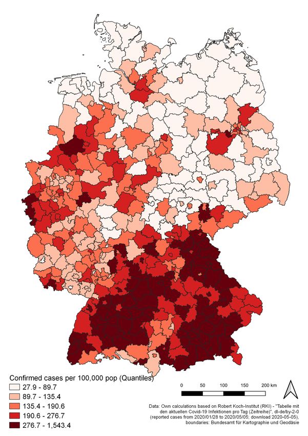
T. Wieland                                                                                 47

                         Figure 1: Logistic growth of an epidemic

(2020a), Chowell et al. (2014) and Tsoularis (2002). Unlike exponential growth, logistic
growth includes two stages, allowing for a saturation effect. The first stage is characterized
by an exponential growth of infections due to an unregulated spreading of the disease. As
more infections accumulate, the number of at-risk susceptible persons decreases because of
immunization, death, or behavioral changes as well as public health interventions. After
the inflection point of the infection curve, when the infection rate is at its maximum, the
growth decreases and the cumulative number of infections approximate its theoretical
maximum, which is the saturation value (see Figure 1).
    In the logistic growth model, the cumulative number of infected or diseased persons
at time t, C(t) is a function of time:

                                                C0 S
                             C(t) =                                                       (1)
                                      C0 + (S − C0 ) exp (−rSt)

where C0 is the initial value of C at time 0, r is the intrinsic growth rate, and S is the
saturation value.
   The infection rate is the first derivative:
                                     dC            C
                                         = rC 1 −                                      (2)
                                     dt             S
    The inflection point of the logistic curve indicates the maximal infection rate before
the growth declines, which means a flattening of the cumulative infection curve. The
inflection point, ip, is equal to:
                                                S
                                           ip =                                        (3)
                                                2
at time
                                                   c
                                          tip =                                           (4)
                                                  rS
where:
                                                  C0
                                       c = ln                                             (5)
                                                C − C0
  When empirical data (here: time series of cumulative infections) is available, the three
model parameters r, S and C0 can be estimated empirically.

                                                       REGION : Volume 7, Number 2, 2020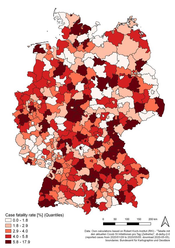
48                                                                                  T. Wieland

   We fit the models in a three-step estimation procedure including both OLS (Ordinary
Least Squares) and NLS (Nonlinear Least Squares) estimation. The former is used for
generating initial values for the iterative NLS estimation, making use of the linearization
and stepwise parametrization of the logistic function. Following Engel (2010), the
nonlinear logistic model (Equ. 1) can be transformed into a linear model (on condition
that the saturation value is known) by taking the reciprocal on both sides, taking natural
logarithms and rearranging the function:
                                    1   1        S − C0
                             ln(       − ) = ln(        ) − rSt                              (6)
                                   C(t) S         SC0
The transformed dependent variable, yi∗ , can be expressed by a linear relationship with
two parameters, the intercept (b̂) and slope (m̂):
                                                   1   1
                                      yi∗ = ln(       − )                                    (7)
                                                  C(t) S
                                          ŷ ∗ = b̂ + m̂t                                    (8)
    In step 1, an approximation of the saturation value is estimated, which is necessary for
the linear transformation of the model. Transforming the empirical values C(t) according
to Equ. (7), we have a linear regression model (Equ. 8). By utilizing bisection (Kaw et al.
2011), the best value for S is searched minimizing the sum of squared residuals. The
bisection procedure consists of 10 iterations, while the start values are set around the
current maximal value of C(t) (Interval: [max(C(t)) + 1; max(C(t)) ∗ 1.2]).
    The resulting preliminary start value for the saturation parameter, Ŝstart , is used in
step 2. We transform the observed C(t) using Equ. (7) with the preliminary value of Ŝ
from step 1, Ŝstart . Another OLS model is estimated (Equ. 8). The estimated coefficients
are used for calculating the start values of r̂ and Ĉ0 for the nonlinear estimation (Engel
2010):
                                                       m̂
                                        r̂start = −                                      (9)
                                                     Ŝstart
and
                                                     Ŝstart
                                 Ĉ0start =                                             (10)
                                               1 + Ŝstart exp (b̂)
In step 3, the final model fitting is done using Nonlinear Least Squares (NLS), while
inserting the values from steps 1 and 2, Ŝstart , Ĉ0start and r̂start , as start values for the
iterative process. The NLS fitting uses the default Gauss-Newton algorithm (Ritz, Streibig
2008) with a maximum of 500 iterations.
    Using the estimated parameters r̂, Ĉ0 and Ŝ, the inflection point of each curve is
calculated via equations (3) to (5). The inflection point tip is of unit time (here: days)
and assigned to the respective date tipdate (YYYY-MM-DD). Based on this date, the
following day tipdate+1 is the first day after the inflection point at which time the infection
rate has decreased again. For graphical visualization, the infection rate is also computed
using Equ. (2).

2.2   Estimating the dates of infection
In the present study, we use the daily updated data on confirmed SARS-CoV-2/COVID-19
cases, provided by federal authorities, the German Robert Koch Institute (RKI) (RKI
2020b). This dataset includes all persons who have been tested positive on the SARS-
CoV-2 virus using a PCR (polymerase chain reaction) test and reported from local health
authorities to the RKI. However, one must consider that neither the volume of tests nor
the criteria for conducting a test are constant over time: Up to and including May 2020,
almost exclusively people with acute respiratory symptoms were tested for SARS-CoV-2,
as, with few exceptions, the presence of relevant symptoms is an exclusion criterion for
testing in the RKI guidelines for medical doctors (IBBS 2020). In other words, this testing
policy is targeted at the disease (COVID-19), not the virus (SARS-CoV-2). Thus, most
of the cases in the present data are COVID-19 sufferers, whilst asymptomatic infected

REGION : Volume 7, Number 2, 2020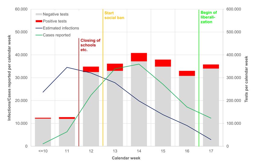
T. Wieland                                                                                                49

people and individuals with milder course are underrepresented. In the vast majority of
cases, the date of onset of symptoms is reported in the dataset as well (an der Heiden,
Hamouda 2020). The test volume was increased heavily from calendar week 11 (127,457
tests) to 12 (348,619 tests) but remains in the same order of magnitude until calendar
week 18 (300,000-400,000 tests per week) (RKI 2020c).
    The dataset used here is from May 5, 2020 and includes 163,798 cases. This data
includes information about age group, sex, the related place of residence (county) and
the date of report (Variable Meldedatum). The reference date in the dataset (Variable
Refdatum) is either the day the disease started, which means the onset of symptoms, or
the date of report (an der Heiden, Hamouda 2020). The date of onset of symptons is
reported in the majority of cases (108,875 and 66.47%, respectively).
    The date of infection, which is of interest here, is either unknown or not included in
the official dataset. Thus, it is necessary to estimate the approximate date of infection
dependent on two time periods: the time between the infection and the onset of symptons
(incubation period) and the delay between onset of symptoms and official report (reporting
delay). From the 108,875 cases where the onset of the symptoms is known, we can calculate
the mean reporting delay as 6.84 days. Additionally, we assume an incubation period
of five days. This is a rather conservative assumption (which means a relatively short
time period) referring to the current epidemiological estimates (see Table 2). In their
model-based scenario analysis towards the total number of diseases and deaths, the RKI
also assumes an average incubation period of five days (an der Heiden, Buchholz 2020).
Taking into account incubation period and reporting delay, there is an average all-over
delay between infection and reporting of about 12 days (see Figure 2).
    But this is just one side of the coin. As an inspection of the case data reveals, the delay
differs by case characteristics (age group, sex) and counties. In their current prognosis,
the RKI estimates the dates of onset of symptoms by Bayesian nowcasting based on the
reporting date, but not taking into account the incubation time. The RKI nowcasting
model incorporates delays of reporting depending on age group and sex, but not including
spatial (county-specific) effects (an der Heiden, Hamouda 2020). Exploring the dataset
used here, we see obvious differences in the reporting delay with respect to age groups
and sex. There seems to be a tendency of lower reporting delays for young children and
older infected individuals (see Table 3). Taking a look at the delays between onset of
symptoms and reporting date on the level of the 412 counties (not shown in table), the
values range between 2.39 days (Würzburg city) and 17.0 days (Würzburg county).

                  Figure 2: Time between infection and reporting of case

     Table 2: Studys estimating the incubation period of SARS-CoV-2/COVID-19

 Study                  n       Distribution Mean (CI95)          SD (CI95)        Median (CI95) Min. Max.
 Backer et al. (2020)   88       Weibull           NA            2.3 (1.7, 3.7)    6.4 (5.6, 7.7)   NA   NA
 Lauer et al. (2020)    181     Lognormal          5.5           1.52 (1.3, 1.7)   5.1 (4.5, 5.8)   NA   NA
 Leung (2020)         175 (a)    Weibull    1.8   (1.0,   2.7)        NA                NA          NA   NA
                      175 (b)    Weibull    7.2   (6.1,   8.4)        NA                NA          NA   NA
 Li et al. (2020)       10      Lognormal   5.2   (4.1,   7.0)        NA                NA          NA   NA
 Linton et al. (2020)   158     Lognormal   5.6   (5.0,   6.3)   2.8 (2.2, 3.6)    5.0 (4.4, 5.6)    2   14
 Sun et al. (2020)       33        NA              4.5                NA                NA          NA   NA
 Xia et al. (2020)      124      Weibull    4.9   (4.4,   5.4)        NA                NA          NA   NA

Notes: (a) = Travelers to Hubei, (b) = Non-Travelers. Source: own compilation.

                                                                 REGION : Volume 7, Number 2, 2020
50                                                                                            T. Wieland

  Table 3: Delay between onset of symptoms and official report by age group and sex

     Age group          Sex                            Delay between onset of symptoms and
                                                               reporting date [days]
                                                       Mean                   SD
     A00-A04            female                         5.82                          5.68
     A05-A14            female                         6.09                          5.34
     A15-A34            female                         6.82                          5.59
     A35-A59            female                         7.00                          5.98
     A60-A79            female                         7.08                          6.22
     A80+               female                         5.10                          5.83
     unknown            female                         8.71                          9.79
     A00-A04            male                           5.93                          5.98
     A05-A14            male                           6.04                          5.12
     A15-A34            male                           6.78                          5.52
     A35-A59            male                           7.18                          5.90
     A60-A79            male                           7.20                          6.14
     A80+               male                           5.70                          5.84
     unknown            male                           9.86                          8.42
     A00-A04            unknown/diverse                3.50                          2.39
     A05-A14            unknown/diverse                4.00                          5.20
     A15-A34            unknown/diverse                6.44                          4.87
     A35-A59            unknown/diverse                6.95                          5.51
     A60-A79            unknown/diverse                7.36                          5.87
     A80+               unknown/diverse                6.50                          11.40
     unknown            unknown/diverse                9.60                          3.58
                   all-over                            6.84                          5.90

Source: own calculation based on data from RKI (2020b). Note: The date of onset of symptoms is known
for 108,875 (66.47%) of 163,798 cases in the dataset.

    For the estimation of the dates of infection, it is necessary to distinguish between
the cases where the date of symptom onset is known or not. In the former case, no
assumption must be made towards the delay between onset of symptoms and date report.
The calculation is simply:
                                       ˆ i = do i − incp
                                      di                                                   (11)
       ˆ i is the estimated date of infection of case i, do i is the date of onset of symptoms
where di
reported in the RKI dataset and incp is the average incubation period equal to five (days).
    For the 54,923 cases without information about onset of symptoms, we estimate this
delay based on the 108,875 cases with known delays. As the reporting delay differs
between age group, sex and county, the following dummy variable regression model is
estimated (stochastic disturbance term is not shown):
                               A−1
                               X                       S−1
                                                       X                  C−1
                                                                          X
               ˆ asc = α +
               ds                    βa Dagegroupa +         γs Dsexs +         δc Dcountyc         (12)
                                a                       s                  c

       ˆ asc is the estimated delay between onset of symptoms and report depending on
where ds
age group a, sex s and county c, Dagegroupa is a dummy variable indicating age group
a, Dsexs is a dummy variable indicating sex s, Dcountyc is a dummy variable indicating
county c, A is the number of age groups, S is the number of sex classifications, C is the
number of counties and α, β, γ and δ are the regression coefficients to be estimated.
   Taking into account the delay estimation, if the onset of symptoms is unknown, the
date of infection of case i is estimated via:
                                      ˆ i = dr i − ds
                                      di           ˆ asc − incp                                     (13)
where dr i is the date of report in the RKI dataset.

REGION : Volume 7, Number 2, 2020
T. Wieland 51
2.3 Models of regional growth rate and mortality
To test which variables predict the intrinsic growth rate and the regional mortality of
SARS-CoV-2/COVID-19, respectively, two regression models were estimated. In the first
model with the intrinsic growth rate r as dependent variable, we include the following
predictors:
• In the media coverage about regional differences with respect to COVID-19 cases
in Germany, several experts argue that a lower population density and a higher
share of older population reduce the spread of the virus, with the latter effect being
due to a lower average mobility (Welt online 2020b). It is well known that human
mobility potentially increases the spread of an infectious disease. Also work-related
commuting and tourism are considered as drivers of virus transmission (Charaudeau
et al. 2014, Dalziel et al. 2014, Findlater, Bogoch 2018). To test these effects, four
variables are included into the model: 1) The population density (POPDENS ),
2) the share of population of at least 65 years (POPS65 ), 3) an indicator for the
intensity of commuting (CMI ) formulated by Guth et al. (2010), and 4) the number
of annual tourist arrivals per capita (TOUR) for each county. All variables were
calculated based on official statistics for the most recent year (2018/2019) (Destatis
2020a,b,c).
• In the media coverage, the lower prevalence in East Germany is also explained by
1) a different vaccination policy in the former German Democratic Republic and 2)
a lower affinity towards carnival events as well as 3) less travelling to ski resorts
due to lower incomes (Welt online 2020b). Thus, a dummy variable (1/0) for East
Germany is included in the model (EAST ).
• We test for the influence of different governmental interventions by including dummy
variables for the states (“Länder”) Bavaria (BV ), Saarland (SL), Saxony (SX ) and
North Rhine Westphalia (NRW ), as well as Baden-Wuerttemberg (BW ). Unlike
the other 13 German states, the first three states established a curfew additional to
the other measures at the time of phase 3, as is identified in the present study. Like
Bavaria, North Rhine Westphalia and Baden-Wuerttemberg belong to the “hotspots”
in Germany, with the latter state having a prevalence similar to Bavaria. Saxony
has a prevalence below the national average (RKI 2020a).
• Apart from any interventions, when a disease spreads over time, also the susceptible
population must decrease over time. As more and more individuals get infected
(maybe causing temporal or lifelong immunization or, in other cases, death), there
are continually fewer healthy people to get infected (Li 2018) (see also Section 2.1).
Consequently, regional growth must decrease with increasing regional prevalence
and over time (and vice versa). In the specific case of SARSCoV-2/COVID-19, the
outbreak differs between German counties (starting with “hotspots” like Heinsberg
or Tirschenreuth county). Differences in growth may be due to different periods of
time the virus is present and differences in the corresponding prevalence. Thus, two
control variables are included in the model, the county-specific prevalence (PRV )
and the number of days since the first (estimated) infection (DAYS ).
In the second model for the explanation of regional mortality (MRT ), five more
independent variables have to be incorporated:
• From the epidemiological point of view, the “risk group” of COVID-19 for severe
courses (and even deaths) is defined as people of 60 years and older. The arithmetic
mean of deceased attributed to COVID-19 is equal to 81 years (median: 82 years).
Out of 6,831 reported deaths on May 5 2020, 6,524 were of age 60 or older (95.51%).
This is, inter alia, because of outbreaks in residential homes for the elderly (RKI
2020a). Thus, the raw data from the RKI (RKI 2020b) was used to calculate the
share of confirmed infected individuals of age 60 or older in all infected persons
for each county (INFS60 ), which is included into the regression model for regional
mortality.
REGION : Volume 7, Number 2, 202052 T. Wieland
• Several health-specific variables are found to influence the mortality risk (as well
as the risk of severe course) of COVID-19. These individual-specific risk factors
include, inter alia, diabetes, obesity, other respiratory diseases, or smoking (Engina
et al. 2020, Selvan 2020). There are several possible health indicators which are
unfortunately not available for German counties. Thus, the average health situation
is captured by incorporating the average regional life expectancy into the model
(LEXP ), which is made available by the German Federal Institute for Research on
Building, Urban Affairs and Spatial Development (BBSR 2020).
• On the regional level, air pollution was found to be a contributing factor to COVID-
19 fatality (Ogen 2020, Wu et al. 2020). According to Wu et al. (2020), the regional
air pollution with respect to particulate matter (annual mean of daily PM 10 values,
unit: µg/m3 ) is included into the model (PM10 ). Since Ogen (2020) shows a
correlation between nitrogen dioxide concentration and COVID-19 fatality, this type
of air pollution (annual mean of daily NO 2 values, unit: µg/m3 ) is incorporated
into the model as well (NO2 ). Both air quality indicators are made available by
the German Environment Agency (UBA 2020a) on the level of single monitoring
stations. These stations are available geocoded (UBA 2020b) and have been assigned
to the German counties via a nearest neighbor join. Thus, the county-level values
of both indicators equal the values of the nearest monitoring station.
• The intrinsic growth rate of each county is incorporated into the model as well.
Considering the chronology of an infectious disease spread, there must be a reciprocal
relationship between growth speed and mortality: The more individuals die in the
context of the regarded disease, the fewer susceptibles are left to be infected, resulting
in a deceleration of the pandemic spread (Li 2018) (see also Section 2.1). Thus,
there must be a negative correlation between mortality and growth rate, all other
things being equal. Consequently, the county-specific intrinsic growth rate (r) is
included as control variable.
See Table 4 for all variables included into the models. All continuous variables,
including the dependent variables (r and MRT, respectively), were transformed via
natural logarithm in the regression analysis. This leads to an interpretation of the
regression coefficients in terms of elasticities and semi-elasticities (Greene 2012). Two
variants were estimated for the growth rate model (with and without dummy variables)
and three for the mortality model (with and without growth rate as well as a third model
including both growth rate and dummy variables). The minimum significance level was
set to p ≤ 0.1. In the first step, the regression models were estimated using an Ordinary
Least Squares (OLS) approach and tested with respect to multicollinearity using variance
inflation factors (VIF ) with a critical value equal to five (Greene 2012).
However, SARS-CoV-2/COVID-19 cases are obviously not evenly distributed across
all German counties as the disease spread started in a few “hotspots” in Bavaria, Baden-
Wuerttemberg and North Rhine Westphalia (RKI 2020a, Tagesspiegel 2020b). Of course,
an infectious disease can be transmitted across county borders, in particular, by contact
between residents of one region and a nearby region. As a consequence, it is to be
expected that indicators of disease spread – such as the regarded variables growth rate
and mortality – are similar between nearby regions. Thus, further model-based analyses
require considering possible spatial autocorrelation in the dependent variables (Griffith
2009). Consequently, both dependent variables were tested for spatial autocorrelation
using Moran’s I-statistic and the model estimation was repeated using a spatial lag
model. In this type of regression model, spatial autocorrelation is modeled by a linear
relationship between the dependent variable and the associated spatially lagged variable,
which is a spatially weighted average value of the nearby objects. The influence of spatial
autocorrelation is captured by adding a further parameter, ρ, to the regression equation,
which is also tested for significance. Spatial linear regression models are not fitted by
OLS but by Maximum Likelihood (ML) estimation. Both Moran’s I and the spatial lag
model require a weighting matrix to define the proximity of the regarded spatial object to
nearby objects (Chi, Zhu 2008, Rusche 2008). Here, the weighting matrix for the spatial
object (county i) was defined as all adjacent counties.
REGION : Volume 7, Number 2, 2020T. Wieland 53
Table 4: Variables in the regression models for growth rate and mortality
Variable Calculation/unit Data source
r Intrinsic growth rate see Section 2.1 own calculation based on
RKI (2020b)
Di
MRT Mortality cumulative popi
∗ 100000 own calculation based on
(Porta 2008) RKI (2020b), Destatis (2020b)
Ci
PRV Prevalence cumulative popi
∗ 100000 own calculation based on
(Porta 2008) RKI (2020b), Destatis (2020b)
DAYS Time since first days (discrete) own calculation based on
infection RKI (2020b)
popi
POPDENS Population density Ai
own calculation based on
Destatis (2020b)
pop65+i
POPS65 Share of population popi
∗ 100 own calculation based on
age 65 or older Destatis (2020b)
CMouti +CMini
CMI Intensity of commuting Lresi +Lwork
own calculation based on
i
(Guth et al. 2010) Destatis (2020c)
Ti
TOUR Tourist density popi
∗ 1000 own calculation based on
Destatis (2020a,b)
C60+i
INFS60 Share of infected age Ci
∗ 100 own calculation based on
60 or older in all RKI (2020b)
infected persons
LEXP Life expectancy years (mean) BBSR (2020)
PM10 Air pollution PM 10 µg/m3 (annual mean) UBA (2020a,b)
NO2 Air pollution NO 2 µg/m3 (annual mean) UBA (2020a,b)
EAST Dummy for East Germany 1=East Germany, else 0
BV Dummy for Bavaria 1=Bavaria, else 0
SL Dummy for Saarland 1=Saarland, else 0
SX Dummy for Saxony 1=Saxony, else 0
NRW Dummy for North Rhine 1=North Rine West-
Westphalia phalia, else 0
BW Dummy for Baden-Wuert- 1=Baden-Wuerttem-
temberg berg, else 0
Note: Ci is the cumulative number of reported SARS-CoV-2/COVID-19 cases in county i, Di is the
cumulative number of reported deaths attributed to COVID-19 in county i, C60+i is the cumulative
number of reported infected persons of age 60 or older in county i, emphpopi is the population of county
i, Ai is the area of county i, emphpop65+i is the number of inhabitants of county i of age 65 or older,
emphCMemphouti and CMini is the number of commuters from and to county i, respectively, Lemphresi
and Lemphworki is the number of employees whose place of residence is county i and whose place of work
is county i, respectively.
2.4 Software
The analysis in this study was executed in R (R Core Team 2019), version 3.6.2. The
parametrization of logistic growth models was done using own functions for the OLS
estimation based on the description in Engel (2010) and the nls() function for the final
NLS estimation. For the steps of the regression analyses and presentation of results, the
packages car (Fox, Weisberg 2019), REAT (Wieland 2019), spdep (Bivand et al. 2013),
and stargazer (Hlavac 2018) were used. For creating maps, QGIS (QGIS Development
Team 2019), version 3.8, was used, including the plugin NNJoin (Tveite 2019) for one
further analysis.
3 Results
3.1 Estimation of infection dates and national inflection point
Figure 3 shows the estimated dates of infection and dates of report of confirmed cases
and deaths for Germany. The curves are not shifted exactly by the average delay period
REGION : Volume 7, Number 2, 202054 T. Wieland
(a) Daily cases (b) Cumulative cases
Figure 3: Reported SARS-CoV-2 infections in Germany over time (dates of report vs.
estimated dates of infection)
Source: own illustration.
Data source: own calculations based on RKI (2020b)
Table 5: Date of inflection point depending on assumed incubation period
Study Median of incubation Date of inflection point
time (CI-95) Lower Median Upper
Linton et al. (2020) 5.0 (4.4, 5.6) 2020-03-20 2020-03-20 2020-03-19
Backer et al. (2020) 6.4 (5.6, 7.7) 2020-03-20 2020-03-19 2020-03-17
Source: own calculation based on data from RKI (2020b).
because of the different delay times with respect to case characteristics and county. The
average time interval between estimated infection and case reporting is x̄ = 11.92 [days]
(SD = 5.21). When applying the logistic growth model to the estimated dates of infection
in Germany, the inflection point for Germany as a whole is on March 20, 2020.
Before switching to the regional level, we take into account the statistical uncertainty
resulting from the estimation of the infection dates. About one third of the delay values
for the time between onset of symptoms and case reporting was estimated by a stochastic
model. Furthermore, the estimates of SARS-CoV-2/COVID-19 incubation period differ
from study to study. This is why in the present case a conservative – which means a
small – value of five days was assumed. Thus, we compare the results when including
1) the 95% confidence intervals of the response from the model in Equ. (12), and 2) the
95% confidence intervals of the incubation period as estimated by Linton et al. (2020).
Figure 4 shows three different modeling scenarios, the mean estimation and the lower
and upper bound of incubation period and delay time, respectively. The lower bound
variant incorporates the lower bound of both incubation period and delay time, resulting
in smaller delay between infection and case reporting and, thus, a later inflection point.
The upper bound shows the counterpart. On the basis of the upper bound, the inflection
point is already on March 19. Using the higher values of incubation period estimated by
Backer et al. (2020), the upper bound results in an inflection point on March 17, while
the lower bound variant leads to the turn on March 20. Considering confidence intervals
of incubation period and delay time, the inflection point for the whole of Germany can
be estimated between March 17 and March 20, 2020 (see Table 5).
REGION : Volume 7, Number 2, 2020T. Wieland 55
Figure 4: Estimated logistic growth model (including inflection point) for cumulative
SARS-CoV-2 infections in Germany (based on estimated dates of infection) incorporating
upper and lower bounds (95%-CI)
Source: own illustration. Data source: own calculations based on RKI (2020b)
3.2 Estimation of growth rates and inflection points on the county level
Figure 5 shows the estimated intrinsic growth rates (r) for the 412 counties. Figure 6
provides six examples of the logistic growth curves with respect to four counties identified
as “hotspots” (Tirschenreuth, Heinsberg, Greiz and Rosenheim) and two counties with a
low prevalence (Flensburg and Uckermark). There are obvious differences in the growth
rates, following a spatial trend: The highest growth rates can be found in counties in
North Germany (especially Lower Saxony and Schleswig-Holstein) and East Germany
(especially Mecklenburg-Western Pomerania, Thuringia and Saxony). To the contrary,
the growth rates in Baden-Wuerttemberg and North Rine Westphalia appear to be quite
low. Taking a look at the time since the first estimated infection date in the German
counties (see Figure 7a), the growth rates tend be much smaller the longer since the
disease appeared in the county.
The regional inflection points indicate the day with the local maximum of infection rate.
From this day forth, the exponential disease growth turns into degressive growth. In Figure
7b, the dates of the first day after the regional inflection point are displayed. The dates are
categorized according to the coming into force of relevant nonpharmaceutical interventions
(see Table 1). Table 6 summarizes the number of counties and the corresponding population
shares by these categories. Figure 8 shows the intrinsic growth rate (y axis) and the day
after the inflection point (colored points) against time (x axis). Figure 9 shows the same
information against regional prevalence (x axis).
In 255 of 412 counties (61.89%) with 54.58 million inhabitants (65.66% of the national
population), the SARS-CoV-2/COVID-19 infections had already decreased before phase
3 of measures came into force on March 23, 2020. In a minority of counties (51, 12.38%),
Table 6: German counties by first day after inflection point
First day after inflection point Counties [no.] Counties [%] Population [Mill.] Population [%]
Before March 13 6 1.46 0.98 1.17
March 13 to March 16 45 10.92 8.27 9.95
March 17 to March 20 138 33.50 31.03 37.33
March 21 to March 22 66 16.02 14.30 17.20
March 23 to April 19 157 38.11 28.54 34.34
Sum 412 100 83.13 100
Source: own illustration. Data source: own calculations based on RKI (2020b)
REGION : Volume 7, Number 2, 202056 T. Wieland
Figure 5: Intrinsic growth rate by county
the curve already flattened before the closing of schools and child day care centers (March
16-18, 2020). Six of them exceeded the peak of new infections even before March 13. This
category refers to the appeals of chancellor Merkel and president Steinmeier on March
12. In 157 counties (38.11%) with a population of 28.54 million people (34.34% of the
national population), the decrease of infections took place within the period of strict
regulations towards social distancing and ban of gatherings.
The average time interval between the first estimated infection and the respective
inflection point of the county is x̄ = 30.32 [days]. However, the time until inflection point
is characterized by a large variance (SD = 11.92), but this may be explained partially by
the (de facto unknown) variance in the incubation period and the variance in the delay
between onset of symptoms and reporting date.
In all counties, the inflection points lie between March 6 and April 18, 2020, which
means a time period of 43 days between the first and the last flattening of a county’s
epidemic curve. The first regional decrease can be found in Heinsberg county (North
Rhine Westphalia; 254,322 inhabitants), which was one of the first Corona “hotspots”
in Germany. The estimated inflection point here took place at March 6, 2020, leading
to a date of the first day after the inflection point of March 7. The latest estimated
inflection point (April 18, 2020) took place in Steinburg county (Schleswig-Holstein;
131,347 inhabitants).
As Figure 8 shows, the intrinsic growth rates, which indicate an average growth level
over time, and inflection points of the logistic models are linked. Growth speed declines
REGION : Volume 7, Number 2, 2020T. Wieland 57
(a) Tirschenreuth county (Bavaria) (b) Heinsberg county (North Rhine Westphalia)
(c) Greiz county (Thuringia) (d) Rosenheim county (Bavaria)
(e) Uckermark county (Brandenburg) (f) Flensburg (Schleswig-Holstein)
Figure 6: Cumulative SARS-CoV-2 infections (based on estimated dates of infection) and
estimated logistic growth models (including infection rate and inflection point) in six
German counties
Source: own illustration. Data source: own calculations based on RKI (2020b)
REGION : Volume 7, Number 2, 2020T. Wieland
REGION : Volume 7, Number 2, 2020
Figure 7: Time since first infection by county (left) and First day after inflection point by county (right)
58T. Wieland 59
Figure 8: Growth rate and first day after inflection point vs. time
Source: own illustration. Data source: own calculations based on RKI (2020b)
Figure 9: Growth rate and first day after inflection point vs. prevalence
Source: own illustration. Data source: own calculations based on RKI (2020b)
over time (see also Figures 5 and 8), more precisely, it declines in line with the time
the disease is present in the regarded county (Pearson correlation coefficient of -0.47,
p < 0.001). The longer the time between inflection point and now, the lower the growth
speed, and vice versa. This process takes place over all German counties with a time
delay depending on the first occurrence of the disease. As shown in Figure 9, there is also
a negative correlation between regional prevalence and growth rate (Pearson correlation
coefficient of -0.722, p < 0.001). These relationships, which are closely linked to the
chronology of an infectious disease spread and the characteristics of the logistic growth
model, respectively, are included into the regression models as control variables.
3.3 Regression models for intrinsic growth rates and mortality
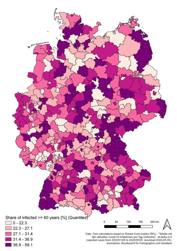
The variables of most interest used within the models are mapped in Figures 10a (preva-
lence, PRV ), 10b (mortality, MRT ) and 11a (share of infected individuals of age ≥ 60,
POPS65 ). Additionally, Figure 11b shows the current case fatality rate on the county
level. Tables 7 and 8 show the estimation results for the OLS regression models explaining
the intrinsic growth rates and the mortality, respectively, both transformed via natural
logarithm. Table 9 displays the Moran’s I-statistic for the dependent variables of the two
models. Tables 10 and 11 show the estimation results for the spatial lag models.
In all of the OLS models, no variable exceeded the critical value of VIF ≥ 5. For the
prediction of the intrinsic growth rate, two model variants were estimated without and
with the state dummy variables (Table 7). From the aspect of explained variance, the
second OLS model provides a better fit (R2 = 0.731 and Adj.R2 = 0.723, respectively)
REGION : Volume 7, Number 2, 2020T. Wieland
REGION : Volume 7, Number 2, 2020
Figure 10: Prevalence by county (left) and Mortality by county (right)
60T. Wieland
Figure 11: Share of reported infected individuals of age 60 and older by county (left) and CFR by county (right)
REGION : Volume 7, Number 2, 2020
6162 T. Wieland
Table 7: Estimation results for the growth rate model (OLS)
Dependent variable: ln(r)
(1) (2)
ln (POPDENS) −0.177∗∗∗ −0.102∗∗∗
(0.028) (0.027)
ln (POPS65) 0.830∗∗∗ 1.165∗∗∗
(0.284) (0.269)
ln (CMI) 0.607∗∗∗ 0.420∗∗∗
(0.091) (0.087)
ln (TOUR) 0.146∗∗∗ 0.035
(0.042) (0.041)
EAST −0.087 −0.045
(0.091) (0.089)
BV 0.473∗∗∗
(0.091)
SL 0.118
(0.231)
SX −0.580∗∗∗
(0.168)
NRW −0.428∗∗∗
(0.097)
BW 0.011
(0.108)
ln (PRV) −0.911∗∗∗ −1.039∗∗∗
(0.049) (0.056)
DAYS −0.019∗∗∗ −0.014∗∗∗
(0.003) (0.003)
Constant −3.660∗∗∗ −4.214∗∗∗
(1.144) (1.079)
Observations 412 412
R2 0.678 0.731
Adjusted R2 0.672 0.723
Residual Std. Error 0.587 0.540
Degrees of Freedom 404 399
F Statistic 121.278∗∗∗ 90.307∗∗∗
Degrees of Freedom 7; 404 12; 399
Note: pT. Wieland 63
SARS-CoV-2/COVID-19 is present in the county, the growth speed declines on average by
1.4%. Here, one has to keep in mind that these relationships are reciprocal and represent
the mandatory decline of susceptible individuals over time.
For the prediction of mortality (MRT ), the growth rate (r) and the state dummy
variables (BV, SL, SX and NRW ) are entered into the model analyis successively, resulting
in the three models shown in Table 8. When comparing models 1 and 2, adding the growth
rate as independent variable increases the explained variance substantially (Adj.R2 = 0.219
and 0.367, respectively). The third model provides the best fit, adjusted for the number
of explanatory variables (Adj.R2 = 0.383). No significant influence can be found for the
spatial (POPDENS ), demographic (POPS65 ), mobility (PI and TOUR), and air pollution
variables (PM10 and NO2 ). Life expectancy (LEXP ) and the dummy for East German
counties (EAST ) are only significant in the first model. However, the share of infected
people of age ≥ 60 (INFS60 ) significantly increases the regional mortality: An increase
in the share of people of the “risk group” in all infected by 1% increases the mortality
by approx. 0.5%. The only significant state-specific effect is found for Bavaria: The
mortality in Bavarian counties is higher than in the counties of other states. Furthermore,
a two-sample t-test reveals that Bavarian counties have a significantly higher share of
infected belonging to the risk group (x̄ = 31.11%) compared to the remaining states
(x̄ = 29.28%), with a difference of 1.83 percentage points (p = 0.054). The reciprocal
relationship between mortality and growth rate is also significant.
As expected, spatial autocorrelation can be detected among the dependent variables.
The Moran’s I-statistic for both regional growth rate and mortality (0.49 and 0.16,
respectively) is significant (see Table 9). Consequently, the OLS estimations are expected
to be biased. Therefore, we apply a spatial lag model in the next step.
With respect to the spatial lag model for regional growth rates (Table 10), the ρ-
parameter in both model variants is significant (ρ = 0.158 and ρ = 0.095, respectively),
which indicates a significant spatial lag effect. However, when comparing the second
spatial lag model (with AIC = 674.96, which is superior to model 1 with AIC = 733.37)
to the second OLS model (see Table 7), there are only negligible differences in the
parameter estimates and significance levels: The same independent variables are found
to be significantly correlated with growth rates. They also have the same sign, which
indicates the same direction of influence. Intrinsic growth rates on the county level are
predicted by population density (approx. -0.9), population share of 65 and older (approx.
1.1), commuting intensity (approx. 0.4), and state-specific dummy variables (Bavaria:
approx. 0.5, Saxony: approx. -0.5, North Rhine Westphalia: approx. -0.4) as well as the
control variables (Prevalence: approx. -1.0 and time since first infection: approx. -0.01).
The same conclusion can be drawn with respect to the spatial lag models for mortality
(Table 11), when comparing them to the OLS models (Table 8). The spatial lag effect
is only significant in the first model (ρ = 0.165) but not in models 2 (ρ = 0.042) and 3
(ρ = −0.044). Regional mortality is significantly influenced by the share of infected people
of age ≥ 60 (approx. 0.5) and the dummy variable for Bavarian counties (approx. 1.2) as
well as correlated with regional growth rates (approx. -1.6). As spatial autocorrelation
was also detected for the regional growth rate, which is an independent variable in the
mortality models, a further robustness check of the estimations is necessary: Table 12
shows the results for the second and third mortality model in a spatial Durbin model,
which incorporates a spatial lag effect for both the dependent variable (ρ) and the regional
growth rate (lag ln (r)). The lag effect of ln(r) is statistically significant, but the other
results remain qualitatively the same (share of infected people of age ≥ 60: approx. 0.5;
dummy variable for Bavarian counties: approx. 1).
With respect to the regression models for regional growth and mortality, the results
of the OLS estimations were confirmed by those from the models allowing for spatial
autocorrelation. Although there is obvious spatial autocorrelation (which can be explained
plausibly by interregional transmission of the infectious disease), both OLS and spatial
regression models show nearly the same results with respect to strength and direction
of correlations. From the spatial statistic point of view, this can be explained with
the incorporated independent variables as regional differences in both growth rate and
mortality are predicted entirely by the interregional variation in causal factors.
REGION : Volume 7, Number 2, 202064 T. Wieland
Table 8: Estimation results for the mortality model (OLS)
Dependent variable: ln (MRT+0.0001)
(1) (2) (3)
ln (POPDENS) −0.060 −0.268∗∗ −0.148
(0.132) (0.121) (0.124)
ln (POPS65) −0.738 0.883 1.730
(1.316) (1.196) (1.230)
ln (CMI) −0.627 0.397 0.025
(0.412) (0.385) (0.396)
ln (TOUR) −0.265 0.066 −0.081
(0.188) (0.173) (0.178)
ln (LEXP) 54.205∗∗∗ 11.409 12.349
(12.259) (11.877) (12.556)
ln (PM10) 0.053 −0.226 −0.200
(0.716) (0.645) (0.653)
ln (NO2) 0.428 0.178 0.213
(0.287) (0.259) (0.259)
ln (INFS60+0.0001) 0.618∗∗∗ 0.459∗∗∗ 0.462∗∗∗
(0.104) (0.095) (0.094)
EAST −0.980∗∗ −0.496 −0.148
(0.395) (0.359) (0.385)
BV 1.110∗∗∗
(0.334)
SL 0.800
(0.983)
SX −0.909
(0.738)
NRW −0.144
(0.433)
BW 0.193
(0.465)
DAYS 0.017 −0.014 −0.011
(0.013) (0.012) (0.012)
ln (r) −1.570∗∗∗ −1.535∗∗∗
(0.161) (0.171)
Constant −237.384∗∗∗ −62.529 −69.684
(55.406) (53.006) (55.923)
Observations 412 412 412
R2 0.238 0.384 0.407
Adjusted R2 0.219 0.367 0.383
Residual Std. Error 2.596 2.336 2.308
Degrees of Freedom 401 400 395
F Statistic 12.525∗∗∗ 22.679∗∗∗ 16.916∗∗∗
Degrees of Freedom 10; 401 11; 400 16; 395
Note: ∗ pT. Wieland 65
Table 10: Estimation results for the growth rate model (spatial lag model)
Dependent variable: ln(r)
(1) (2)
ln (POPDENS) −0.151∗∗∗ −0.089∗∗∗
(0.027) (0.027)
ln (POPS65) 0.755∗∗∗ 1.119∗∗∗
(0.279) (0.265)
ln (CMI) 0.561∗∗∗ 0.402∗∗∗
(0.092) (0.087)
ln (TOUR) 0.121∗∗∗ 0.024
(0.041) (0.041)
EAST −0.148∗ −0.076
(0.089) (0.089)
BV 0.498∗∗∗
(0.090)
SL 0.096
(0.226)
SX −0.538∗∗∗
(0.166)
NRW −0.368∗∗∗
(0.100)
BW 0.073
(0.110)
ln (PRV) −0.827∗∗∗ −1.002∗∗∗
(0.058) (0.060)
DAYS −0.018∗∗∗ −0.014∗∗∗
(0.003) (0.003)
Constant −2.677∗∗ −3.562∗∗∗
(1.159) (1.110)
ρ 0.158∗∗∗ 0.095∗
(0.049) (0.050)
Observations 412 412
Log Likelihood −356.682 −322.481
σ2 0.329 0.280
Akaike Inf. Crit. 733.365 674.962
LR Test (df = 1) 9.283∗∗∗ 3.193∗
Wald Test (df = 1) 10.325∗∗∗ 3.608∗
Note: ∗ pYou can also read