FlowReg: Fast Deformable Unsupervised Medical Image Registration using Optical Flow
←
→
Page content transcription
If your browser does not render page correctly, please read the page content below
Journal of Machine Learning for Biomedical Imaging. 2021:0. pp 1-46       Submitted 1/2021; Published TBA/2021

                                             FlowReg: Fast Deformable Unsupervised Medical Image
                                                       Registration using Optical Flow*

                                         Sergiu Mocanu                                                                                smocanu@ryerson.ca
                                         Electrical, Computer, and Biomedical Engineering, Ryerson University, Toronto, ON, Canada
                                         Alan R. Moody                                                                         alan.moody@sunnybrook.ca
                                         Department of Medical Imaging, University of Toronto, Toronto, ON, Canada
                                         April Khademi                                                                                akhademi@ryerson.ca
                                         Electrical, Computer, and Biomedical Engineering, Ryerson University, Toronto, ON, Canada.
arXiv:2101.09639v1 [cs.CV] 24 Jan 2021

                                         Keenan Research Center for Biomedical Science, St. Michael’s Hospital, Unity Health Network, Toronto, ON, Canada.
                                         Institute for Biomedical Engineering, Science and Technology (iBEST), a partnership between St. Michael’s Hospital
                                         and Ryerson University, Toronto, ON, Canada.

                                                                                           Abstract

                                              In this work we propose FlowReg, a deep learning-based framework that performs unsu-
                                              pervised image registration for neuroimaging applications. The system is composed of two
                                              architectures that are trained sequentially: FlowReg-A which affinely corrects for gross
                                              differences between moving and fixed volumes in 3D followed by FlowReg-O which per-
                                              forms pixel-wise deformations on a slice-by-slice basis for fine tuning in 2D. The affine
                                              network regresses the 3D affine matrix based on a correlation loss function that enforces
                                              global similarity between fixed and moving volumes. The deformable network operates on
                                              2D image slices and is based on the optical flow network FlowNet-Simple but with three
                                              loss components. The photometric loss minimizes pixel intensity differences differences,
                                              the smoothness loss encourages similar magnitudes between neighbouring vectors, and a
                                              correlation loss that is used to maintain the intensity similarity between fixed and moving
                                              image slices. The proposed method is compared to four open source registration techniques
                                              ANTs, Demons, SE, and Voxelmorph for FLAIR MRI applications. In total, 4643 FLAIR
                                              MR imaging volumes (approximately 255, 000 image slices) are used from dementia and vas-
                                              cular disease cohorts, acquired from over 60 international centres with varying acquisition
                                              parameters. To quantitatively assess the performance of the registration tools, a battery
                                              of novel validation metrics are proposed that focus on the structural integrity of tissues,
                                              spatial alignment, and intensity similarity. Experimental results show FlowReg (FlowReg-
                                              A+O) performs better than iterative-based registration algorithms for intensity and spatial
                                              alignment metrics with a Pixelwise Agreement (PWA) of 0.65, correlation coefficient (R)
                                              of 0.80, and Mutual Information (MI) of 0.29. Among the deep learning frameworks evalu-
                                              ated, FlowReg-A or FlowReg-A+O provided the highest performance over all but one of the
                                              metrics. Results show that FlowReg is able to obtain high intensity and spatial similarity
                                              between the moving and the fixed volumes while maintaining the shape and structure of
                                              anatomy and pathology.

                                              Keywords: Registration, unsupervised, deep learning, CNNs, neuroimaging, FLAIR-
                                              MRI, registration validation

                                         ©2021 1-46. License: CC-BY 4.0.
                                         https://www.melba-journal.org/article/XX-AA.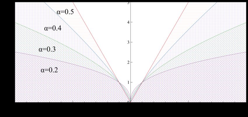
Mocanu et al.

Figure 1: Left: FLAIR MRI slice showing hyperintense WML in the white matter, dark
          cerebrospinal fluid (CSF) in the ventricles and intracranial cavity, and the brain.
          Right: Registration of a moving image M (x, y) (green) to the fixed image F (x, y)
          (purple) space.

1. Introduction
Magnetic resonance imaging (MRI) offers non-invasive visualization of soft tissue that is
ideal for imaging the brain. The etiology and pathogenesis of neurodegeneration, and
the effects of treatment options have been heavily investigated in T1, T2, Proton Den-
sity (PD), Diffusion Weighted (DW), and Fluid-Attenuated Inversion Recovery (FLAIR)
MR sequences (Udaka et al., 2002)(Hunt et al., 1989)(Sarbu et al., 2016)(Trip and Miller,
2005)(Guimiot et al., 2008) for dementia (Oppedal et al., 2015) and Alzheimer’s Disease
(AD) (Kobayashi et al., 2002). As cerebrovascular disease (CVD) has been shown to be a
leading cause of dementia, there is growing interest into examining cerebrovascular risk fac-
tors in the brain using neuroimaging. CVD markers, such as white matter lesions (WML),
predict cognitive decline, dementia, stroke, death, and WML progression increases these
risks (Debette and Markus, 2010), (Alber et al., 2019). WML represent increased and al-
tered water content in hydrophobic white matter fibers and tracts. Changes in white matter
vasculature likely contributes to WML pathogenesis (Gorelick et al., 2011). Research into
the vascular contributions to dementia and neurodegeneration could be valuable for devel-
oping new therapies (Frey et al., 2019), (Alber et al., 2019), (Griffanti et al., 2018), (Malloy
et al., 2007). FLAIR MRI is preferred for WML analysis (Wardlaw et al., 2013) (Badji and
Westman, 2020) since the usual T2 high signal from cerebrospinal fluid (CSF) is suppressed,
highlighting the white matter disease (WMD) high signal. This is due to increased water
content secondary to ischemia and demyelination and much more robustly seen in FLAIR
than with T1 and T2 sequences (Lao et al., 2008), (Khademi et al., 2011), (Kim et al.,
2008), Piguet et al. (2005). See Figure 1 for an example slice from a FLAIR MRI imaging
volume, exhibiting hyperintense WML.
    To adequately assess the evolution of neurodegenerative disease, neuroimages of pa-
tients from multicentre datasets are needed to adequately represent diverse populations

                                               2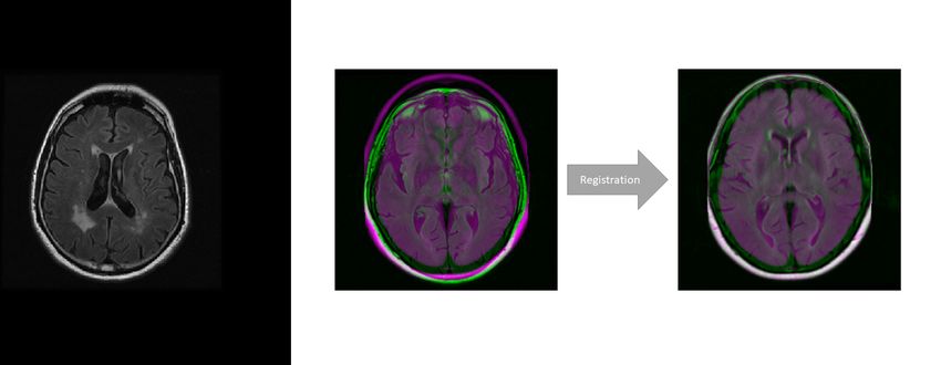
FlowReg: CNN Registration

and disease. However, manual analysis on a large scale is impractical, labourious, subjec-
tive, and error prone. In contrast, image analysis and machine learning tools can alleviate
these challenges by automatically analyzing neuroimaging data objectively, efficiently, and
robustly.
    One family of algorithms heavily relied upon in neuroimaging research is image registra-
tion. Image registration is the process of aligning two images (one fixed and one moving)
so these images are in the same geometric space after registration. An example registration
is shown in Figure 1 which shows the fixed and moving images are not aligned originally,
but after registration, the two images have maximal correspondence. The benefit is that
structures and changes between two images can be directly compared when images are
registered. For this reason, image registration has played an important role in analyzing
large neuroimaging data repositories to align longitudinal scans of the same patient to as-
sess disease change over time (Csapo et al., 2012), (El-Gamal et al., 2016), map patient
images to an atlas for template-based segmentation (Iglesias and Sabuncu, 2015), (Phellan
et al., 2014), or to correct for artifacts such as patient motion and orientation (Mani and
Arivazhagan, 2013). As medical images are composed of highly relevant anatomical and
pathological structures such as brain tissue, ventricles, and WMLs, it is important that
the shape and relative size of each structure is maintained in the registered output. MR
images are highly complex so obtaining correspondence while maintaining structural and
anatomical integrity presents a challenging task.
    Traditionally, the process of registration, or aligning two images has been framed as
an optimization problem, which searches for the transform T between a moving (Im ) and
a fixed (If ) image by optimizing some similarity criteria between the fixed and moving
images. The transformation function T could consist of affine transformation parameters
such as translation, rotation and scale. For each iteration, the transformation is applied to
the moving image, and the similarity between the fixed and moving images is calculated via
a cost function C. The transform may be found by iteratively optimizing the cost function,
as in:
                                T = arg max C (If , T (Im )) .                            (1)
                                           T

This optimization is typically calculated via gradient descent and ends when maximum sim-
ilarity is found or a maximum number of iterations is obtained. A variety of cost functions
have been used in the literature, with the most popular ones being mutual information
(MI), cross-correlation (CC), and mean-squared error (MSE) (Maes et al., 1997) (Avants
et al., 2008). Registrations can be done globally via affine transformation or on a per-pixel
level through the use of non-uniform deformation fields (each pixel in the moving image has
a target movement vector). Once a transformation has been calculated, the image is regis-
tered by applying this transformation to the moving image. Transformations can typically
be classified as rigid and non-rigid. Rigid transforms include rotations and translations, and
preserve angles and edge lengths between pixels, while non-rigid transforms may warp an
image by scaling and shearing. Transformations can be applied on two-dimensional medical
images or three-dimensional volumes to perform spatial alignment. Registration is typically
performed between a moving image and a template atlas space, longitudinal intra-patient
data, or inter-patient scans.

                                               3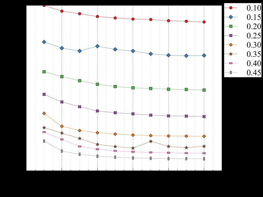
Mocanu et al.

    Registration algorithms that involve an iterative-based approach calculate an appropri-
ate deformation parameter to warp a moving image to the fixed geometric space (Avants
et al., 2008; Pennec et al., 1999; Johnson et al., 2013; Klein et al., 2010). These algorithms
aim to minimize a dissimilarity metric at every iteration through gradient descent. The
main downside of such approaches is that the process is computationally expensive and
any calculated characteristics are not saved after an intensive computational procedure; the
transformation parameters are discarded and not used for the next pair of images. In large
multi-centre datasets this can create various challenges, including large computation times
or non-optimal transformations. To overcome the non-transferable nature of traditional im-
age registration algorithms, machine learning models that learn transformation parameters
between images have been gaining interest in the research communities (Cao et al., 2017)
(Sokooti et al., 2017) (Balakrishnan et al., 2018). During test time, the model is applied to
transform (register) unseen image pairs.
    Recently, several convolutional neural network-based (CNN) medical image registration
algorithms have emerged to address the non-transferable nature, lengthy execution and
high computation cost of the classic iterative-based approaches (Balakrishnan et al., 2018;
Uzunova et al., 2017). In 2017, researchers adapted an optical flow CNN model, FlowNet
(Dosovitskiy et al., 2015), to compute the deformation field between temporally spaced
images (Uzunova et al., 2017). Although promising, this approach required ground truth
deformation fields during training, which is intractable for large clinical datasets. To over-
come these challenges, Voxelmorph was developed as a completely unsupervised CNN-based
registration scheme that learns a transformation without labeled deformation fields (Jader-
berg et al., 2015). In another work, Zhao et al. (2019) proposed a fully unsupervised method
based on CNNs that includes cascaded affine and deformable networks to perform align-
ment in 3D in one framework. This work is inspired by these pioneering works but instead
an affine alignment is performed in 3D first, followed by a 2D fine-tuning on slice-by-slice
basis.
    In medical imaging registration applications for neuroimaging, both global and local
alignment is necessary. Global differences such as head angle or brain size can vary signifi-
cantly between patients and these global differences are likely to be mainly realized in 3D.
Additionally, there are local differences arising from variability in the sulci or gyri, or other
fine anatomical differences that are more visible on a per slice basis. Therefore, to get max-
imal alignment between neuroimages, both global differences in 3D and local differences in
2D should be addressed. Other design considerations include dependence on ground truth
data which is impractical or impossible to obtain for large datasets. Lastly, and impor-
tantly, registration algorithms must maintain the structural integrity of important objects
such as WML and ventricles. Additionally, the presence of WML can negatively affect reg-
istration algorithms (Sdika and Pelletier, 2009), (Stefanescu et al., 2004) so it is important
to measure performance with respect to pathology.
    To this end, this paper proposes a CNN-based registration method called FlowReg:
Fast Deformable Unsupervised Image Registration using Optical Flow that addresses these
design considerations in a unified framework. FlowReg is composed of an affine network
FlowReg-A for alignment for gross head differences in 3D and a secondary deformable reg-
istration network FlowReg-O that is based on the optical flow CNNs (Ilg et al., 2017) (Yu
et al., 2016) for fine movements of pixels in 2D, thus managing both global and local differ-

                                               4
FlowReg: CNN Registration

ences at the same time. In contrast to previous works that perform affine and deformable
registration strictly in 3D, we postulate that performing affine registration in 3D followed
by a 2D refinement will result in higher quality registrations for neuroimages. The frame-
work is based on CNNs that learn transformation parameters from many image pairs, that
can be applied to future unseen image pairs. It is fully unsupervised, and ground truth
deformations and transformations are not required which speeds up learning and imple-
mentation. The loss functions are modified and fine-tuned to ensure optimized performance
for neuroimaging applications. Lastly, this framework does not require preprocessing such
as brain extraction and is applied to the whole head of neuroimaging scans.
    FlowReg-A is a novel affine model that warps the moving volume using gross global
parameters to align rotation, scale, shear, and translation to the fixed volume. A 3D
approach is used for the affine model (i.e. volume registration) to ensure coarse differences
are corrected in 3D. A correlation loss that encourages global alignment between the moving
and the fixed volumes is employed to regress the affine parameters. FlowReg-A corrects for
the large differences in 3D prior to deformation in 2D using FlowReg-O. FlowReg-O is
an optical flow-based CNN network from the video processing literature that is adapted
to neuroimaging in this work. It provides for 2D alignment via (small) individual vector
displacements for each pixel on a slice-by-slice basis. The total loss function is tuned and a
novel correlation loss is introduced into the total loss function to enforce global similarity.
    As an additional contribution, a battery of validation tests are proposed to evaluate
the quality of the registration from a clinically salient perspective. Validation of registra-
tion performance is not a simple task and many methods have employed manually placed
landmarks (Balakrishnan et al., 2018), (Uzunova et al., 2017), (de Vos et al., 2019). In med-
ical imaging, whether the anatomy and pathology in the moving images have maintained
their structural integrity and intensity properties is of interest, while obtaining maximum
alignment with the fixed image. To measure these effects, several novel metrics are pro-
posed to measure the performance as a function of three categories: structural integrity,
spatial alignment, and intensity similarity. Structural (tissue) integrity is measured via vol-
umetric and structural analysis with the proportional volume (PV), volume ratios ∆V and
surface-surface distance (SSD) metrics. Spatial alignment is measured via pixelwise agree-
ment (PWA), head angle (HA) and dice similarity coefficient (DSC). Intensity similarity
is measured using traditional metrics: mutual information (MI) and correlation coefficient
(Pearson’s R) as well as one additional new one, the mean-intensity difference (MID).
    Using the validation metrics, FlowReg is compared to four established and openly avail-
able image registration methods: Demons (Thirion, 1995, 1998; Pennec et al., 1999), Elastix
(Klein et al., 2010), ANTs (Avants et al., 2008), and Voxelmorph (Balakrishnan et al., 2018).
Three are traditional non-learning iterative based registration methods while Voxelmorph
is a CNN-based registration tool. Performance is measured over a large and diverse multi-
institutional dataset collected from over 60 imaging centres world wide of subjects with
dementia (ADNI) (Mueller et al., 2005) and vascular disease (CAIN) (Tardif et al., 2013).
There are roughly 270,000 images and 4900 imaging volumes in these datasets with a range
of imaging acquisition parameters. The rest of the paper is structured as follows: Section
2.1 describes the novel FlowReg architecture, which is comprised of affine (FlowReg-A) and
optical flow (FlowReg-O) models, and Section 2.2 outlines the validation metrics. The data

                                              5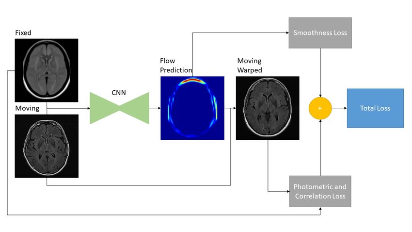
Mocanu et al.

Figure 2: FlowReg is composed of an affine (FlowReg-A) and an optical flow (FlowReg-O)
          component.

used, experimental setup, and results are discussed in Section 3 followed by the discussions
and conclusions in Section 4 and Section 5.

2. Methods

In this section, we introduce FlowReg, Fast Deformable Unsupervised Image Registration
using Optical Flow, with focus on neuroimaging applications. Given a moving image volume
denoted by M (x, y, z), where M is the intensity at the (x, y, z) ∈ Z 3 voxel, and the fixed
image volume F (x, y, z) the system automatically learns the registration parameters for
many image pairs, and uses that knowledge to predict the transformation T for new testing
images. The transformation T is learned through deep learning models and applied to
the original images to result in an aligned image. The section closes with a battery of
novel registration validation metrics focused on structural integrity, intensity and spatial
alignment that can be used to measure registration performance.

2.1 FlowReg

FlowReg, is based exclusively on CNN-based architectures, and the alignment is fully unsu-
pervised, meaning that we train to regress the registration parameters without ground truth
knowledge. Registration with FlowReg is completed with the two phase approach shown
in Fig. 2. The first component FlowReg-A is a novel 3D affine registration network that
corrects for global differences between the fixed and moving volumes. The second phase
refines the affine registration results on a per slice basis through FlowReg-O, a 2D optical
flow-based registration method inspired from the video processing field (Dosovitskiy et al.,
2015), (Ilg et al., 2017), (Garg et al., 2016), (Yu et al., 2016). To train the two phase ap-
proach, first the affine component is trained, and the affine parameters are obtained for each
volume. Once all the volumes are registered using the affine components, the FlowReg-O
training regimen begins to obtain the deformation fields. The held out test set is used to
test the full FlowReg pipeline end-to-end.

                                              6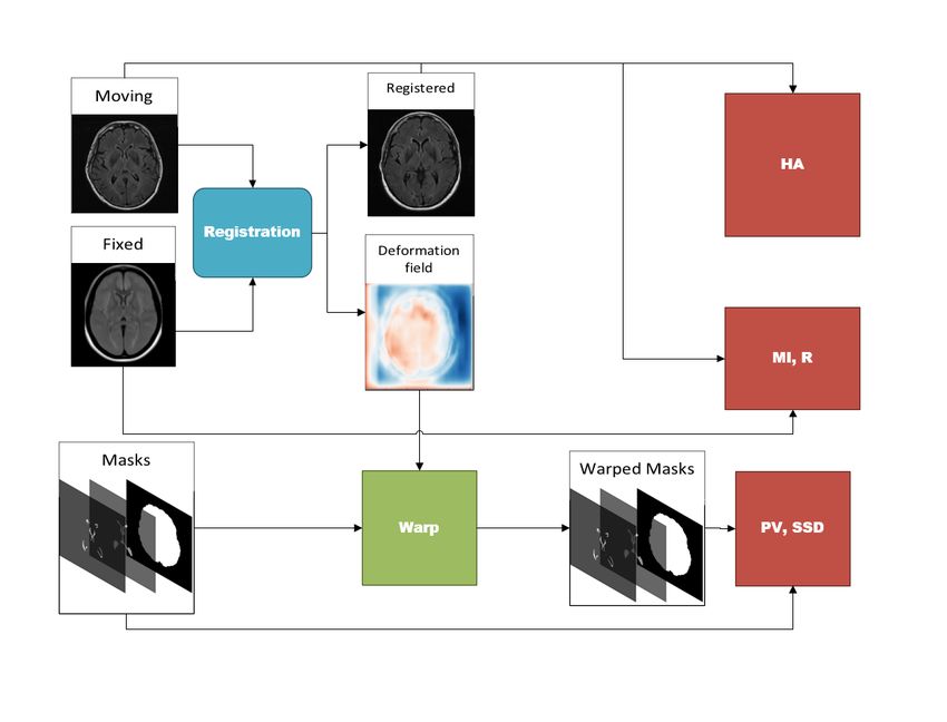
FlowReg: CNN Registration
concatenation
of input
32 16 8
64 512
16
8
128 256
32
128
256
64
64
12
8
12
32 fc
1
6
25
6
25
2 16
Figure 3: Flowreg-A model structure. A pair of 3D input volumes are concatenated, each
yellow box represents the output of 3D convolutional layers, the numbers at the
bottom of the box are the number of feature maps generated by each convolutional
kernel. The last layer (purple) is a fully connected layer with 12 nodes and a linear
activation function.
2.1.1 FlowReg-A: Affine Registration in 3D
The proposed affine model FlowReg-A warps the moving volume using gross global pa-
rameters to align head rotation, scale, shear, and translation to the fixed volume. This
is beneficial when imaging the brain in 3D, since each patient’s head orientation or head
angle can vary in a database. Additionally, images are often of different physical dimen-
sions depending on the scanner type and parameters used for acquisition. To normalize
the global differences such as scale, rotation and translation between the fixed and moving
image volumes, we propose a completely unsupervised 3D affine registration method (i.e.
volume registration) that is based on a CNN, where the transformation parameters are
learned.
The CNN network used to regress the translation, scale, and rotation parameters is
shown in Figure 3 and described in Table 1. In this work, the affine model is comprised
of six convolutional layers and one fully-connected layer. The network has an encoder and
decoder arm where the last layer is a fully connected layer which is used to regress the
flattened version of the three-dimensional affine matrix, A:
a b c d
A = e f g h , (2)
i j k l
where A contains the rotation, scale, and translation parameters. Given this affine trans-
formation matrix, the original image volume may be transformed by Mw (x, y, z) = A ×
M (x, y, z).
7Mocanu et al.
Table 1: FlowReg-A model, details of architecture in Figure 3.
Layer Filters Kernel Stride Activation
fixedInput - - - -
movingInput - - - -
concatenate - - - -
conv3D 16 7x7x7 2, 2, 1 ReLu
conv3D 32 5x5x5 2, 2, 1 ReLu
conv3D 64 3x3x3 2, 2, 2 ReLu
conv3D 128 3x3x3 2, 2, 2 ReLu
conv3D 256 3x3x3 2, 2, 2 ReLu
conv3D 512 3x3x3 2, 2, 2 ReLu
flatten - - - -
dense 12 - - Linear
To solve for the transformation parameters A, a correlation loss was used to encourage
an overall alignment of the mean intensities between the moving and the fixed volumes:
PN
i=1 Fi − F Mwi − Mw
`corr3D (F, Mw ) = 1 − qP 2 qPN 2 (3)
N
i=1 Fi − F i=1 Mwi − Mw
where F is the fixed volume, Mw is the moving volume warped with the calculated matrix,
N is the number of voxels in the volume, Fi is the ith element in F , Mwi is the ith element
in Mw , and F , Mw are the mean intensities of the fixed and moving volumes, respectively.
Using the correlation loss function, the parameters are selected during training that ensures
global alignment between the fixed and moving image volumes.
2.1.2 FlowReg-O: Optical Flow-based Registration in 2D
In this section, the optical flow component of the registration framework, FlowReg-O, will
be described, which performs fine-tuning of the affine registration results on a slice-by-slice
basis (i.e. in 2D). FlowReg-O is adapted from the original optical flow FlowNet architecture,
which was presented for video processing frameworks. Optical flow is a vector field that
quantifies the apparent displacement of a pixel between two temporally separated images.
A video is composed of a number of frames at a certain frame-rate per second, Fs and the
optical flow measures the motion between objects and pixels across frames. Optical flow
can also be used to calculate the velocity of different objects in a scene (Horn and Schunck,
1981). For the task of medical image registration, instead of aligning neighbouring frames,
we will be aligning moving and fixed images. The same principles as the original optical
flow framework are adopted here, where the displacement vector is found and used to warp
pixels between moving and fixed images in 2D.
The original network structure of FlowNet (Dosovitskiy et al., 2015), is composed of
an encoder and decoder arm similar to U-Net (Ronneberger et al., 2015). The encoder
arm is composed of several convolutional layers that reduce the resolution of the image,
but are able to encode various features with each level of convolution. This is a coarse-to-
8FlowReg: CNN Registration
fine approach, where feature maps are able to encode the local and global features in one
framework. Through skip-connections, the model, termed FlowNet Simple, concatenates the
large-scale feature maps with the small upscaled features. This technique provides a more
accurate representation of the learned feature maps since both global and local information
are modeled at the same time (Dosovitskiy et al., 2015). The decoder arm upscales the
obtained features so the output is the same size as the input. At various resolutions, the
generated optical flow is used to warp the moving image and then compared to the fixed
image. The Spatial Transformer Network (STN) is used to warp the moving image with the
predicted flow (Jaderberg et al., 2015). The differentiable nature of STNs are particularly
useful for creating the sampling grid and warping the moving image according to the learned
deformation field.
The proposed deformable registration network is similar to the FlowNet Simple archi-
tecture in terms of the convolutional layers, but adapted to grayscale medical image sizes
and content. See Fig 4 for the FlowReg-O architecture, which is also described in Ta-
ble 2. The original FlowNet architecture was implemented on the synthetically generated
dataset ”Flying Chairs” with known optical flow values for ground truths, thus dissimilar-
ities are calculated as a simple endpoint-error (EPE) (Dosovitskiy et al., 2015; Ilg et al.,
2017). Since then, unsupervised methods have been proposed to train optical flow regressor
networks based on a loss that compares a warped image using the regressed flow and its
corresponding target image. between images by warping a subsequent video frames and gen-
erating flow between the two time points (Yu et al., 2016). In medical imaging, the optical
flow ground truths are impossible to obtain, so the same unsupervised principle is adopted
here, but the losses have been conformed for medical images. In addition to photometric
and smoothness loss components which were used in the original work (Yu et al., 2016),
FlowReg-O utilizes an additional correlation loss term, with each loss encouraging overall
similarity between the fixed and moving images while maintaining small 2D movements in
the displacement field. The addition of the correlation loss function is to impose global
intensity constraints on the solution.
The total loss function is a summation of three components: photometric loss `photo to
keep photometric similarity through the Charbonnier function, the smoothness loss `smooth
which ensures the deformation field is smooth (and limits sharp discontinuities in the vector
field), and the correlation loss `corr , which was added to enforce global similarity in the
intensities between the moving and fixed images. The total loss for FlowReg-O is shown
below:
L(u, v; F (x, y), Mw (x, y)) =γ · `photo (u, v; F (x, y), Mw (x, y))+
(4)
ζ · `corr (u, v; F (x, y), Mw (x, y)) + λ · `smooth (u, v)
where u, v are the estimated horizontal and vertical vector fields, F (x, y) is the fixed image,
Mw (x, y) = M (x + u, y + v) is the warped moving image, and γ, ζ, and λ are weighting
hyper-parameters.
The photometric loss, adopted from Yu et al. (2016), is the difference between intensities
of the fixed image and the warped moving image and evaluates to what degree the predicted
optical flow is able to warp the moving image to match the intensities of the fixed image on
9flow256x256
flow128x128
flow64x64
flow32x32
flow16x16
flow8x8
flow4x4
2
2 2
2 2
2 2
2 2
concatenation 2 2
of input 2 2
Mocanu et al.
64
32 32 1024 I/ 32
16 16 512 I/ 1024 I/ 512 512 2 I/ 16
8 8 512 I/ 512 I/ 256 512 2 I
/ 8
4 I/ I/ I/ 4
10
2 I/ 256 512 128 256 2 I/ 2
I/ 256 64 128 2 I/
I I I
128 3264 2
64 1622
2
Figure 4: Flowreg-O model structure. A pair of 2D input images are concatenated, each yellow box represents the output of
2D convolutional layers, the numbers at the bottom of the box are the number of feature maps generated by each
convolutional kernel. Skip connections are shown between the upscaling decoder (blue) arm being concatenated (gray
boxes) with the output of the encoder layers. The flow at seven resolutions are labeled with flow above the corresponding
outputs. I is the input image resolution 256 × 256FlowReg: CNN Registration
Table 2: FlowReg-O model details of architecture in Figure 4.
Layer Filters Kernel Strides Activation
fixedInput - - - -
movingInput - - - -
concatenate - - - -
conv2D 64 7x7 2, 2 L-ReLu
conv2D 128 5x5 2, 2 L-ReLu
conv2D 256 5x5 2, 2 L-ReLu
conv2D 256 3x3 1, 1 L-ReLu
conv2D 512 3x3 2, 2 L-ReLu
conv2D 512 3x3 1, 1 L-ReLu
conv2D 512 3x3 2, 2 L-ReLu
conv2D 512 3x3 1, 1 L-ReLu
conv2D 1024 3x3 2, 2 L-ReLu
conv2D 1024 3x3 1, 1 L-ReLu
conv2D 2 3x3 1, 1 -
upconv2D 2 4x4 2, 2 -
upconv2D 512 4x4 2, 2 L-ReLu
conv2D 2 3x3 1, 1 -
upconv2D 2 4x4 2, 2 -
upconv2D 256 4x4 2, 2 L-ReLu
conv2D 2 3x3 1, 1 -
upconv2D 2 4x4 2, 2 -
upconv2D 128 4x4 2, 2 L-ReLu
conv2D 2 3x3 1, 1 -
upconv2D 2 4x4 2, 2 -
upconv2D 64 4x4 2, 2 L-ReLu
conv2D 2 3x3 1, 1 -
upconv2D 2 4x4 2, 2 -
upconv2D 32 4x4 2, 2 L-ReLu
conv2D 2 3x3 1, 1 -
upconv2D 2 4x4 2, 2 -
upconv2D 16 4x4 2, 2 L-ReLu
conv2D 2 3x3 2, 2 -
resampler - - - -
11Mocanu et al.
Figure 5: Charbonnier function (Eqn. 6) showing the effect of various α values of 0.5, 0.4,
0.3, and 0.2.
a pixel-by-pixel basis:
1 X
`photo (u, v;F (x, y), Mw (x, y)) = ρ(F (i, j) − Mw (i, j))) (5)
N
i,j
where N is the number of pixels and ρ is the Charbonnier penalty function which is used
to reduce contributions of outliers. The Charbonnier penalty is defined by:
ρ(x) = (x2 + 2 )α (6)
where x = (F − Mw ), is a small value (0.001), and α regulates the difference in intensities
between the moving and fixed images such that large differences can be damped to keep
the magnitudes of the deformation vectors within a reasonable limit. The effect of the α
parameter on the Charbonnier function is shown in Fig. 5. In contrast, for smaller α values,
the Charbonnier function suppresses the output magnitude which is used to regress finer
movements in the displacement field.
The smoothness loss is implemented to regularize the flow field. The loss component
encourages small differences between neighbouring flow vectors in the height and width
directions and is defined by
H X
X W
`smooth (u, v) = [ρ(ui,j − ui+1,j ) + ρ(ui,j − ui,j+1 )+
j i (7)
ρ(vi,j − vi+1,j ) + ρ(vi,j − vi,j+1 )],
where H and W are the number of rows and columns in the image and ui,j and vi,j are
displacement vectors for pixel (i, j) and ρ is the Charbonnier function. This loss measures
12FlowReg: CNN Registration
Figure 6: Overview of loss components for the deformable registration network, FlowReg-O.
the difference between local displacement vectors and minimizes the chances of optimizing
to a large displacement between neighbouring pixels.
Lastly, we added an additional correlation loss component to encourage an overall align-
ment of the mean intensities between the moving and the fixed 2D images (similar to
FlowReg-A), as in:
PN
i=1 Fi − F Mwi − Mw
`corr2D (F, Mw ) = 1 − qP 2 qPN 2 , (8)
N
i=1 F i − F i=1 M wi − M w
where F is the fixed image, Mw is the moving image warped with the calculated flow, N
is the number of pixels in the image, Fi is the ith element in F , Mwi is the ith element in
Mw , and F , Mw are the mean intensities of the fixed and moving images, respectively. A
summary of the loss components and how they are implemented for the FlowReg-O network
is is shown in Fig. 6.
2.2 Validation Metrics
In this section, the proposed performance metrics that will be used to validate registration
performance are described. There are three categories of metrics that each measure a
particular aspect of registration accuracy that have clinical relevance, including: structural
integrity, spatial alignment, and intensity similarity. The specific validation measures for
each category are shown in Table 3 and the flow diagram to compute each of the metrics is
shown in Figure 7. In total, there are nine metrics computed, and each metric is described
further below.
13Mocanu et al.
Figure 7: Registration metrics extraction process. HA = Head Angle, MI = Mutual Infor-
mation, R = Correlation Coefficient, PV = Proportional Volume, SSD = Surface
to Surface Distance.
Table 3: Categories of validation metrics, with respective validation metric computed from
each category.
Category Metric
Structural Integrity Proportional Volume (PV), Volume Ratio (∆Vs ), Surface to Sur-
face Distance (SSD)
Spatial Alignment Head Angle (HA), Pixel-Wise Agreement (PWA), Dice Similarity
Coefficient (DSC)
Intensity Similarity Mutual Information (MI), Correlation Coefficient (Corr), Mean In-
tensity Difference (MID)
14FlowReg: CNN Registration
2.2.1 Structural Integrity: Proportional Volume — PV
If a registration scheme maintains the structural integrity of anatomical and pathological
objects, the relative volume of objects should remain approximately the same after registra-
tion. Using binary masks of anatomical or pathological objects of interest, the proportional
volume (PV) is proposed to measure the volume of a structure (vols ) compared to the total
brain volume (volb ), as in:
vols
PV = . (9)
volb
The volume of objects in physical dimensions is found by multiplying the number of pixels
by voxel resolution:
vol = Vx × Vy × Vz × np , (10)
where vol is the volume in mm3 , Vx and Vy are the pixel width and height and Vz is the
slice-thickness.
The difference between the PV before and after registration can be investigated to
analyze how registration changes the proportion of each structure with respect to the brain.
The difference in PV before and after registration can be measured by
∆P V = P Vorig − P Vreg . (11)
where P Vorig and P Vreg are the PV computed before and after registration. In this work,
two structures of interest are examined for vols : white matter lesions (WML) and ventricles
since these objects are important for disease evaluation. Ideally the ratio of object volumes
to the total brain volume would stay the same before and after registration
2.2.2 Structural Integrity: Volume Ratio — ∆Vs
In addition to the ∆P V which looks at proportional changes in volumes before and after
registration, the volume ratio ∆Vs is also defined on a per object basis. The volume ratio
investigates the volumes of objects before and after registration, as in
volorig
∆Vs = , (12)
volreg
where volorig and volreg are the volumes of object s before and after registration, respec-
tively. The volume ratio is computed for three objects s: the brain, WML and ventricles.
This metric quantifies the overall change in volume before and after registration (the best
ratio is a value equal to 1).
2.2.3 Structural Integrity: Surface to Surface Distance — SSD
A third structural integrity measure, SSD, is proposed to measure the integrity between
objects in the brain before and after registration. In particular, the SSD measures how
the overall shape of a structure changes after registration. To compute the SSD, binary
masks of the brain B(x, y, z), and structure S(x, y, z) of interest are obtained, and an edge
map is obtained to find EB (x, y, z) and ES (x, y, z), respectively. For every non-zero pixel
coordinate (x, y, z) in the boundary of the structure, i.e. ES (x, y, z) = 1, the minimum
Euclidean distance from the structure’s boundary to the brain edge is found. This closest
15Mocanu et al.
surface-to-surface distance between pixels in the objects’ boundaries is averaged over the
entire structure of interest to compute the average SSD
"N #
1 X √
SSD = argmin(xs ,ys ,zs )∈S p+q+r , (13)
N
i=1
where p = (xs − xb )2 , q = (ys − yb )2 , r = (zs − zb )2 are differences between points in the
edge maps of Es and Eb , (xs , ys , zs ) and (xb , yb , zb ) are triplets of the co-ordinates in the
binary edge maps for the structural objects of interest and the brain, respectively, and N
is the number of points in the structure’s boundary. The overall structural integrity of
objects should be maintained with respect to the brain structure after registration, i.e. the
distance between the objects and the brain shape should not be significantly altered. This
metric can be used to investigate the extent in which anatomical shapes are maintained or
distorted by registration by examining the difference in SSD before and after registration
by
SSDorig − SSDreg
∆SSD = , (14)
SSDorig
where SSDorig and SSDreg is the SSD before and after registration, respectively.
2.2.4 Spatial Alignment: Head Angle — HA
Head Angle (HA) is an orientation metric that measures the extent to which the head
is rotated with respect to the midsaggital plane. For properly registered data (especially
for data that is being aligned to an atlas), the HA should be close to zero with the head
being aligned along the midstagittal plane. To measure the HA, a combination of Principal
Component Analysis (PCA) and angle sweep as described in Rehman and Lee (2018);
Liu et al. (2001) is adopted to find the head orientation of registered and unregistered
data. The MRI volume is first binarized using a combination of adaptive thresholding and
opening and closing techniques to approximately segment the head. The coordinates of
each non-zero pixel in this 2D mask are stored in two vectors (one for each coordinate)
and the eigenvectors of these arrays are found through PCA. The directions of eigenvectors
specify the orientation of the major axes of the approximated ellipse for the head region
in a slice with respect to the vertical saggital plane. Eigenvalues are the magnitude of the
eigenvectors (or length of the axes). The largest eigenvalue dictates the direction of the
longest axis which is approximately the head angle θ1 . For improved robustness to outliers
and improve the precision of the estimated angles, a secondary refinement step is utilized
to compute the refined HA θ2 . Every second slice from the middle (axial) slice to the top
of the head are used and the three smallest angles over all slices are taken as candidates
for further refinement.The lowest angles are selected as they are the most representative of
head orientation. Each selected slice is mirrored and rotated according to an angle sweep
from −2 × θ1 < θ2 < 2 × θ1 at 0.5◦ angle increments. At every increment of the rotation,
the cross-correlation between the mirrored rotating image and the original is calculated and
a score is recorded. The angle at which the highest score is selected for the optimized value
θ2 . The final HA is obtained by summing the respective coarse and fine angle estimates,
i.e. θ = θ1 + θ2 .
16FlowReg: CNN Registration
2.2.5 Spatial Alignment: Pixelwise Agreement — PWA
Physical alignment in 3D means that within a registered dataset, each subject should have
high correspondence between slices, i.e. the same slice from each subject should account
for the same anatomy across patients. To measure this effect, a metric called Pixelwise
Agreement (PWA) is proposed. It considers the same slice across all the registered volumes
in a dataset and compares them to the same slice from an atlas template (the fixed volume)
through the mean-squared error. The sum of the error is computed for each slice, to obtain
a slice-wise estimate of the difference between the same slice in the atlas as compared to
each of the same slices from the registered data:
1 1 XX
P W A(z) = (Mj (x, y, z) − F (x, y, z))2 (15)
Nj Nxy
j∈J (x,y)
where z is the slice number for which PWA is computed, Mj (x, y, z) is the moving test
volume j from a total of Nj volumes from the dataset, Nx y is the number of voxels in
slice z and F (x, y, z) is the atlas. Thus, at each slice, for the entire dataset, the PWA
compares every slice to the same slice of the atlas. Low PWA indicates high-degree of
correspondence between all the slices from the registered dataset and that of the atlas and
considers both spatial and intensity alignment. If there is poor spatial alignment, there
will be poor intensity alignment since different tissues will be overlapping during averaging.
1 P
The slice-based PWA may also be summed to get a total volume PWA, i.e. Nz z P W A(z)
where Nz is the number of slices.
2.2.6 Spatial Alignment: Dice Similarity Coefficient — DSC
To further examine spatial alignment, manually delineated brain masks from the moving
volumes M (x, y, z) were warped with the calculated deformation and compared to the brain
mask of the atlas template F (x, y, z) through the Dice Similarity Coefficient (DSC):
2|bM ∩ bF |
DSC = , (16)
|bM | + |bF |
where bM is the registered, moving brain mask and bF is the brain mask of the atlas
template. DSC will be higher when there is a high-degree of overlap between the brain
regions from the atlas and moving volume. For visual inspection of overlap, all registered
brain masks were averaged to summarize alignment accuracy as a heatmap.
2.2.7 Intensity Similarity: Mutual Information — MI
The first intensity-based metric used to investigate registration performance is the widely
adopted Mutual Information (MI) metric that describes the statistical dependence between
two random variables. If there is excellent alignment between the moving and fixed images,
there will be tight clustering in the joint probability mass functions. The MI of two volumes
M (x, y, z) and F (x, y, z) with PMFs of pM (i) and pF (i) is calculated as follows:
p(M,F ) (m, f )
X X
I(M ; F ) = p(M,F ) (m, f ) log (17)
pM (m)pF (f )
f ∈F m∈M
17Mocanu et al.
where p(M,F ) (m, f ) is the joint probability mass function of the intensities of the moving
and fixed volumes, pM (m) is the marginal probability of the moving volume intensities, and
pF (f ) is the marginal probability for the fixed volume.
2.2.8 Intensity Similarity: Pearson Correlation Coefficient — r
The Pearson Correlation Coefficient, r, is used as the second intensity measure which quan-
tifies the correlation between the intensities in the moving M (x, y, z) and F (x, y, z) volumes:
Pn
i=1 (Mi − M )(Fi − F )
r(M, F ) = qP qP (18)
n 2 n 2
i=1 (Mi − M ) i=1 (Fi − F )
where N is the number of voxels in a volume, Mi and Fi are the pixels from the moving
and fixed volumes, and F and M are the respective volume mean intensities.
2.2.9 Intensity Similarity: Mean Intensity Difference — MID
The last registration performance metric considered is the mean intensity difference, MID,
which measures the quality of a newly generated atlas A(x, y, z) compared to the original
atlas (fixed volume). To create the new atlas, the moving volumes M (x, y, z) from a dataset
are registered to the original atlas F (x, y, z) and then the same slices are averaged across the
registered dataset generating the atlas A(x, y, z). The intensity histograms of the original
F (x, y, z) and newly generated atlases A(x, y, z) are compared through the mean square
error to get the MID, as in
1 X
M ID(A, F ) = (pA (i) − pF (i)) (19)
Ni
i
where pF and pA are the probability distributions of the intensities for the fixed (original at-
las) and moving volumes (new atlas) and Ni is the maximum number of intensities. Changes
to the intensity distribution of registered images could arise from poor slice alignment. The
higher the similarity between the new atlas and the original, the lower the error between
the two.
3. Experiments and Results
In this section the data and the experimental results are detailed.
3.1 Data
In this work, we evaluate the performance of FlowReg under a large amount of diverse
medical imaging data. In particular, we focus on neurological FLAIR MRI because of the
potential to identify biomarkers related to vascular disease and neurodegeneration. Over
270,000 FLAIR MR images were retrieved from two datasets which comprises roughly 5000
imaging volumes from over 60 international imaging centres. This comprises one of the
largest FLAIR MRI datasets in the literature that is being processed automatically to the
best of our knowledge. The first dataset is from the Canadian Atherosclerosis Imaging
Network (CAIN) Tardif et al. (2013) and is a pan-Canadian study of vascular disease. The
18FlowReg: CNN Registration
second dataset is from the Alzheimer’s Disease Neuroimaging Initiative (ADNI) (Mueller
et al., 2005) which is an international study for Alzheimer’s and related dementia patholo-
gies. The study and acquisition information is shown in Table 4 and Table 10. Based
on image quality metrics supplied with the ADNI database, scans with large distortions,
motion artifacts, or missing slices, were excluded from the study. In total there were 310
volumes excluded based on this criteria. For training, validation and testing an 80/10/10
data split was employed and volumes were randomly sampled from CAIN and ADNI. The
resulting splits were 3714 training volumes (204,270 images), 465 validation volumes (25,575
images) and 464 test volumes (25,520 images). See Figure 9 for example slices from several
volumes of the ADNI and CAIN test set, exhibiting wide variability in intensity, contrast,
anatomy and pathology.
Table 4: Demographics and imaging information for experimental datasets used in this work
(CAIN and ADNI).
Dataset # Subjects # Volumes # Slices # Centers Age Sex F/M (%)
CAIN 400 700 31,500 9 73.87 ± 8.29 38.0/58.6
ADNI 900 4263 250,00 60 73.48 ± 7.37 46.5/53.5
The ADNI database consisted of images from three MR scanner manufacturers: General
Electric (n = 1075), Phillips Medical Systems (n = 848), and Siemens (n = 2076) with 18
different models in total. In CAIN there is five different models across three vendors with
General Electric (n = 181), Phillips Medical Systems (n = 230), and Siemens (n = 289).
The number of cases per scanner model and vendor are shown in Table 10 along with the
ranges of the acquisition parameters. As can be seen, this dataset represents a diverse
multicentre dataset, with varying scanners, diseases, voxel resolutions, imaging acquisition
parameters and pixel resolutions. Therefore, this dataset will give insight into how each
registration method can generalize in multicentre data.
To measure the validation metrics proposed in Section 2.2, two sets of images are re-
quired. Firstly, all volumes in the test set (464 volumes) are used to compute the intensity
and spatial alignment metrics: head angle (HA), pixel-wise agreement (PWA), dice similar-
ity coefficient (DSC), mutual information (MI), correlation coefficient (Corr), mean intensity
difference (MID). Second, to compute the structural integrity metrics (PV, volume ratio and
SSD metrics), binary segmentation masks of the structures of interest are required and 50
CAIN and 20 ADNI volumes were sampled randomly from the test set for this task. For the
objects of interest, ventricles and WML objects are selected since they represent clinically
relevant structures that characterize neurodegeneration and aging. Manual segmentations
for the ventricular and WML regions were generated by a medical student after training
from a radiologist. These objects are used to examine the structural integrity before and
after registration. To generate brain tissue masks, the automated brain extraction method
from (Khademi et al., 2020) is utilized to segment cerebral tissue in FLAIR MRI.
The atlas used is this work as the fixed volume F (x, y, z) has the dimensions of 256 ×
256 × 55 and is further detailed in (Winkler et al.). The moving image volumes M (x, y, z)
comes from the image datasets described in Table 10 and no pre-processing was done to
19Mocanu et al.
any of the volumes other than resizing M (x, y, z) to the atlas resolution (256 × 256 × 55)
through bilinear interpolation.
3.2 Experimental Setup
FlowReg-A and FlowReg-O models were trained sequentially. First, FlowReg-A is trained
using 3D volume pairs of M (x, y, z) and F (x, y, z) and using the optimized model parame-
ters, the training volume set is affinely registered to the atlas using the found transformation
(Dalca et al., 2018). Subsequently, the globally aligned volumes are used to train FlowReg-
O, on a slice-by-slice basis, using paired moving M (x, y) and fixed F (x, y) images to obtain
the fine-tuning deformation fields in 2D. For FlowReg-A and FlowReg-O the Adam opti-
mizer was used (Kingma and Ba, 2014) with a β1 = 0.9 and β2 = 0.999, and a learning
rate of lr = 10−4 . FlowReg-A training was computed for 100 epochs using a batch size
of four pairs of volumes from M (x, y, z) and F (x, y, z). FlowReg-O was trained using the
globally aligned 2D images for 10 epochs using a batch size of 64 image pairs (2D) at seven
two-dimensional resolutions: 256 × 256, 128 × 128, 64 × 64, 32 × 32, 16 × 16, 8 × 8, and 4 × 4.
The loss hyper-parameters were set as γ = 1, ζ = 1, and λ = 0.5 as per the original optical
flow work Yu et al. (2016). During the testing phase, the deformation field in the last layer
of the decoding arm is used to warp the moving test images as this resolution provides
per pixel movements and is generated at the same resolution of the input image. Before
applying the test data to the system, there is a parameter fine tuning step that is used to
find the α value for the Charbonnier function in FlowReg-O, described in the next section.
Using the trained models for the complete FlowReg pipeline, the testing performance is
compared to that of VoxelMorph, ANTs, Demons and SimpleElastix.
Training for CNN models was performed using a NVIDIA GTX 1080Ti, with Keras
(Chollet et al., 2015) as a backend to Tensorflow (Abadi et al., 2015) for FlowReg-A,
FlowReg-O, and Voxelmorph. ANTs registration was performed in Python using the Sym-
metric Normalization (SyN) with default values (Avants et al., 2008). Demons algorithm
was implemented in Python using SimpleITK (Johnson et al., 2013). Similarly, the Pythonic
implementation of Elastix (Klein et al., 2010) was employed for SimpleElastix (Marstal
et al., 2016) as an add-on to SimpleITK. As a preprocessing step, prior to running Vox-
elmorph, the volumes were first affinely registered using ANTs-Affine. Voxelmorph was
then trained for 37,000 iterations (to avoid observed overfitting) using the same training
dataset utilized for training FlowReg. Voxelmorph performs 3D convolutions, thus resizing
was necessary to keep the output of the decoder the same size as the pooling and upsam-
pling layers. Both the atlas and the moving volumes were resized to 256 × 256 × 64. This
resolution was chosen to be a binary multiple of 2n to ensure that the decoder arm of the
U-net style network is able to rebuild the learned feature maps to the original input size
and warp the volumes accordingly.
To validate the registration methods, the metrics described in Section 2.2 and shown in
Fig. 7 were used. The structural integrity validation metrics (PV, volume ratio and SSD)
used binary masks for the corresponding brain, ventricle, and WML masks and the resultant
deformation field or transformation from each registration method. The PV calculation
includes PV from the ventricles and WMLs with respect to the whole brain volume. The
volume ratio examines how much the volume of each object changes after registration. The
20FlowReg: CNN Registration
SSD is computed between the ventricle surface and the brain surface only; WML are not
included for this metric since small lesion loads and irregular WML boundaries can create
large differences in the SSD which may not be related to overall integrity. Finally, for all
registration methods and all test data, the large-scale metrics are computed: HA, PWA,
DSC, MI, R and MID were calculated between the registered volumes and atlas for all
testing volumes. Warped masks were binarized with a threshold of 0.1 so as to avoid the
non-integer values obtained from interpolation.
3.3 Results
In this section the experimental results will be presented. First, the effect of α on the
Charbonnier penalty function (Equation 6) for the optical flow photometric and smooth loss
functions in FlowReg-O was analyzed since this parameter plays a major role in reducing
over-fitting and overtly large deformations. Using the held out validation set, the value for
α is selected based on the effect this parameter has on the images, which includes visual
analysis of the distortion on the images, the magnitude of the optical flow field as well as
the average flow magnitude. The model with the appropriate α is used to train the final
model for the remainder experiments.
The registration performance of FlowReg-O is studied for α from 0.10 to 0.45 in 0.05
increments. FlowReg-O was trained at each α value individually and the corresponding total
loss values were recorded over 10 epochs as shown in Fig. 8. Each of these models were
saved and the corresponding deformation fields were used to warp the validation dataset.
Example images from the validation dataset are shown in Figure 9 for each α. These images
have variety of contrasts, ventricle sizes and lesion loads which are ideal for analyzing the
effect of α on image quality and distortion. For larger values of α there is more distortion
in the images, i.e. abrupt discontinuities in the brain periphery or smearing in the interior
strcutures of the brain. For values of α ≤ 0.20 there is minimal brain and head distortion
observed with increasing distortion for α > 0.20. The shape of the ventricles are maintained
when α ≤ 0.25. At α > 0.25 the ventricles are adversely distorted (Figure 9), along
with periventricular lesions which were stretched or smeared. The highest distortion is
experienced in the images is for α between 0.3 − 0.45.
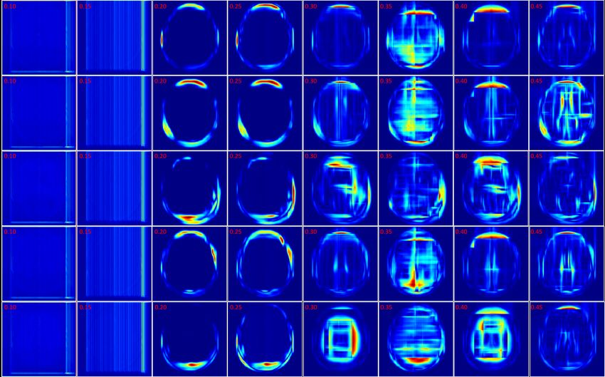
These distortions can be further examined in Figure 10 which investigates the corre-
sponding vector magnitudes of the optical flow for the images in Figure 9. As can be seen,
for high values of α there is abrupt flow magnitudes inside the brain, which corresponds to
the distortion in lesions and ventricles, and there is also large flows at the head boundaries.
For very low α (i.e., 0.1 or 0.15) the flow magnitude is very low indicating minimal pixel
movement. However, at α = 0.2 or α = 0.25 the flow inside the brain is minimized (no
heavy distortions), and pixel movement is mainly on the periphery of the brain and head.
This seems to be the most desirable configuration since there is no distortion of important
clinical features (lesions and ventricles) while offering improved alignment of the boundaries
of the brain and head in 2D.
To examine the flow magnitude for each α over the entire validation set, the average flow
magnitudes per pixel are computed and shown in Figure 11. For α = 0.1 and α = 0.15, on
average, each pixel has a flow magnitude of approximately 0 indicating that the pixels do not
necessarily move. The highest movement is being experienced when α is between 0.3 − 0.45
21Mocanu et al.
Figure 8: The total loss values during training for FlowReg-O at different α values in the
Charbonnier penalty function (Eqn. 6).
which results in more drastic pixel movements in the range of 3 to 6 pixels on average.
These findings are consistent with the appearance of the distorted image slices (Figure 9).
Based on visual inspection of registered volumes, flow magnitude images, and average pixel
movement, the ”sweet-spot” for the α value lies within the 0.2 and 0.25 range. To ensure
there is not any overt movements and to be on the conservative side, we have selected
α = 0.2 for FlowReg-O. The overall effect of FlowReg-A and FlowReg-O with α = 0.2 will
be tested in the reminder of this section.
Using the finalized FlowReg model, test performance will be compared to the registration
performance of each of the comparative methods using the proposed validation metrics. All
of the testing data (464 volumes) were registered using the models and algorithms described
previously. Example registration results for all of the methods are shown in Figure 12. In
this figure, bottom, top and middle slices were chosen to show the spectrum of slices that
need to be accurately warped and transformed from a 3D imaging perspective. In the first
row, slices from the fixed (atlas) volume F (x, y, z) are shown, followed by the corresponding
slices from the moving volume M (x, y, z). The first column contains images with the ocular
orbits and cerebellum in both in the moving and fixed. In the middle slices of the volume,
the ventricles are visible and some periventricular WMLs as well. The top slice of the fixed
volume is the top of the head and is included since it is comprised of small amounts of brain
tissue. The remaining rows display the results of registering the moving images M (x, y, z)
to the fixed images F (x, y, z) for each of the respective tools.
For ANTs registration with the affine and deformable component (SyN) there is good
alignment on the middle slices but the top slice has some pixels missing, and the lower slices
have the ocular orbits in multiple slices (which are not present in the atlas for these slices)
indicating poor alignment in 3D. Demons exhibits large deformations for all three slices and
therefore, this tool is not ideal for clinical applications involving FLAIR MRI. SimpleElastix
seems to align the images over most spatial locations, except the lower slices as they contain
ocular orbits for slices that do not anatomically align with the atlas. Voxelmorph exhibits
22FlowReg: CNN Registration
Figure 9: Single slices from five volumes registered using FlowReg-O at various α values for
the Charbonnier penalty.
23Mocanu et al.
Figure 10: Flow magnitudes of deformation fields from FlowReg-O at various α values.
Images correspond to slices in Figure 9. Blue indicates areas of low flow vector
magnitude and red indicates larger vector magnitude.
Figure 11: The average flow magnitude per pixel for FlowReg-O at various α values over
the validation set.
24You can also read