Haptic Rendering of Arbitrary Serial Manipulators for Robot Programming
←
→
Page content transcription
If your browser does not render page correctly, please read the page content below
Haptic Rendering of Arbitrary Serial Manipulators
                                 for Robot Programming
              Michael Fennel1 , Antonio Zea1 , Johannes Mangler2 , Arne Roennau2 , Uwe D. Hanebeck1

                                                                                                                       planned trajectory
   Abstract— The programming of manipulators is a common                      AR/VR headset
task in robotics, for which numerous solutions exist. In this
work, a new programming method related to the common
master-slave approach is introduced, in which the master is
replaced by a digital twin created through haptic and visual
rendering. To achieve this, we present an algorithm that enables
the haptic rendering of any programmed robot with a serial
manipulator on a general-purpose haptic interface. The results
show that the proposed haptic rendering reproduces the kine-                                   digital twin (DT)
matic properties of the programmed robot and directly provides
the desired joint space trajectories. In addition to a stand-alone
usage, we demonstrate that the proposed algorithm can be                                           haptic robot (HR)           programmed robot (PR)
easily paired with existing visual technology for virtual and                                                 kinematic information
augmented reality to facilitate a highly immersive programming                 other sources                 environment information
experience.
                                                                             Fig. 1. General structure of the proposed digital twin setup for robot
                         I. I NTRODUCTION                                    programming using haptic feedback and virtual/augmented reality.

   The programming of manipulators is a common problem
                                                                             safety issues. In the latter case, each PR type requires its
in robotics and appears in many fields, including industrial
                                                                             own, costly master robot with a matching kinematic structure.
automation, humanoid robots, and even surgical applications.
                                                                             Another variant of programming by demonstration is the
Despite tremendous efforts to abstract and automate the
                                                                             use of a marker (i.e., an object that can be tracked by the
programming and control of robotic manipulators, no uni-
                                                                             programming system) moved by the programmer [1]. Again,
versal approach exists that covers all possible aspects of
                                                                             physical access to the robot environment is required and the
complex problems like painting or assembly. Furthermore,
                                                                             resulting motion might not be compatible with the kinematic
increased sensing capabilities and environmental information
                                                                             constraints of the PR. Additionally, there is no way for the user
in a machine-readable form are required, which are not always
                                                                             to feel interaction forces from the PR and its environment.
available, especially in cost-sensitive applications, complex
                                                                                To overcome these issues while maintaining the idea of
or unstructured environments, or in situations with frequent
                                                                             programming by demonstration, we propose a novel digital
reprogramming. To overcome these issues and to leverage
                                                                             twin (DT) system as depicted in Fig. 1. With this system,
the cognitive capabilities of a human operator or programmer,
                                                                             we leverage existing virtual and augmented reality (VR/AR)
several programming methods are available [1]–[3].
                                                                             techniques in combination with a new method for haptic
   One option is text-based programming, but this requires
                                                                             feedback for the programming of robot motions. To achieve
special knowledge and a high level of abstraction. Beyond
                                                                             this, the kinematic behavior of the arbitrary PR is rendered by
that, it is not guaranteed that a given program with its motions
                                                                             a general-purpose haptic interface, which we will call a haptic
can be executed correctly by the robot due to kinematic and
                                                                             robot (HR). With the proposed solution, the programming
environmental constraints. Another option is programming by
                                                                             person will be enabled to feel and explore properties like
demonstration. In its basic forms, the programmer moves the
                                                                             reach, dexterous workspace, and joint limits of the PR
end effector of the programmed robot (PR) either by directly
                                                                             independent of the visual rendering technology. At the same
touching it or by moving the end effector of a possibly scaled
                                                                             time, undesired properties such as gravity can be removed,
master robot that is linked with the PR acting as a slave.
                                                                             while assistive features can be easily added. Due to the
The disadvantages of both methods are apparent: In the first
                                                                             potential usage of VR/AR, it is not just possible to display
case, physical interaction with the PR is required causing
                                                                             the target environment and the state of the PR, but also to
  1 The authors are with the Intelligent Sensor-Actuator-Systems             give the programming persons a highly immersive feeling.
Laboratory, Institute for Anthropomatics and Robotics, Karlsruhe Institute   Ideally, they will get the impression that they are operating
of Technology, Adenauerring 2, 76131 Karlsruhe, Germany. E-mails:            the PR in its real environment by guiding the end effector
michael.fennel@kit.edu,                   antonio.zea@kit.edu,
uwe.hanebeck@kit.edu                                                         along desired trajectories.
  2 The authors are with the FZI Research Center for Information
Technology, Haid-und-Neu-Str. 10-14, 76131 Karlsruhe, Germany. E-mails:                                II. R ELATED W ORK
mangler@fzi.de, roennau@fzi.de
  This work was supported by the ROBDEKON project of the German                 The application of haptic feedback for path planning or
Federal Ministry of Education and Research.                                  selection tasks is an active topic of research. In [4], an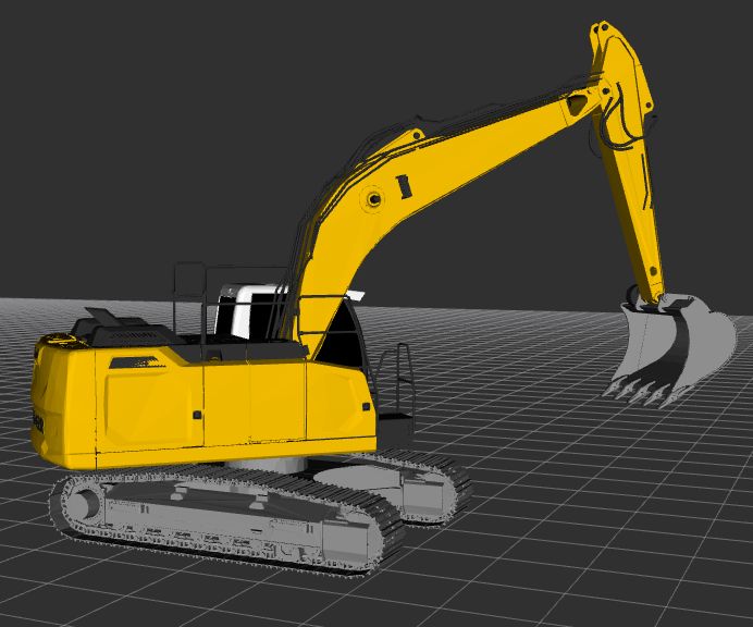
HR                               torques. Superscripts denote the reference coordinate frame in
                                                                     which a quantity is expressed, whereas the subscripts indicate
                        F                                            a point or a pose. For example, pA B represents the position of
               E              DT                                     point B given in coordinates of¯ frame A. To reference the
                                                                     i-th element of a vector, [i] is appended to the subscript. All
                                                                     quantities are given in SI units unless otherwise specified.
                                    R                                   In the remainder, the coordinate frames as illustrated in
                                               H
                                                                     Fig. 2 are used. The frame F denotes the flange of the HR
                                                                     and is assumed to be coincident with the position of its
                                                                     force/torque sensor. The frame H denotes the reference frame
          Fig. 2.   Definition of the used coordinate frames.        of the HR. Moreover, the reference frame of the DT is defined
                                                                     as R and the end effector frame of the DT coincident with
algorithm is presented that supports the user while they             the programmer’s handle is denoted as E.
choose a path, based on a pre-planned, collision-free path
and guiding forces. Kinematic constraints of the PR are not          B. Objective
respected. Another concept for haptic guidance during the               In the following, the PR is assumed to be a serial kinematic
path selection phase for car-like vehicles is given in [5].          structure with n ∈ N+ joints, that are a mixture of prismatic
Although this approach respects the kinematic constraints            and revolute joints. As the PR might be incompatible with
and the limitations of the steering angle, it cannot be applied      the size of the HR or the user, static up- or downscaling is
to other mechanical structures, which disqualifies it for the        allowed. The kinematic model of the scaled PR corresponds
task of rendering kinematics.                                        to the forward kinematics of the DT and is given as
   A more general approach for realizing constraints on a
haptic interface is the so-called virtual fixture as proposed in                               xR = f (q) ,                       (1)
                                                                                               ¯E ¯
[6]. While this approach allows constraining the motion on a                                 qmin ≤ q ≤ qmax .                    (2)
path or surface, it cannot deal with complex manifolds as they                               ¯       ¯ ¯
appear in the workspace description of average manipulators.         Additionally, it is assumed that the linkage, i.e., the point
In [7], a method specifically designed for the haptic rendering      where the user touches the HR to move the end effector of
of surfaces in 3D space is presented. Similar to virtual fixtures,   the DT, and the position of the DT with respect to the HR
this approach is limited to surfaces (i.e., two degrees of           are known and fixed. Formally, this can be expressed with
freedom) and cannot be generalized for more degrees of               the transformations TEF and TH    R.

freedom, making it unsuitable for the haptic rendering of               The HR is any haptic interface, whose dexterous workspace
arbitrary manipulators.                                              is a superset of the DT’s workspace and that accepts Cartesian
                                                                     pose setpoints xH∗   for its flange. Moreover, force and torque
   Independent of haptic feedback, the usage of VR and AR                            ¯F
tools in robotics grew in the last decade due to the increasing      measurements at the flange are available, i.e., fFH and mH    F,
                                                                     are known. Note, that these properties do not      ¯ require¯ a
accessibility of suitable devices [8]. Examples for this are
given in [9] and [10], where robot trajectories are either           manipulator specifically designed as a haptic interface.
recorded in a fully virtual environment or in the real robot            Given these conditions, the goal is now to develop a system,
environment that is augmented with a virtual model of the            that lets the handle attached to the HR behave like the user is
actual robot. The combination of both haptics and VR/AR              moving the real kinematic structure of the PR. This requires
was demonstrated recently for the application example of                1) a haptic rendering algorithm for a kinematic structure
welding robots [11]. Although the idea presented therein is                 defined by (1) and (2), and
independent of a priori environmental knowledge, it does not            2) a visual rendering of the DT in AR or VR.
take into account the kinematic limitations of the robot.            This paper mainly deals with the former, whereas the visual
   As of this writing, we are not aware of any system for robot      rendering is covered only briefly. Interested readers are
programming that combines haptic feedback with VR/AR                 therefore invited to refer to [12] for detailed information
and that respects all kinematic constraints of the PR.               about the visual rendering.

                    III. P ROBLEM S TATEMENT                                IV. H APTIC R ENDERING OF M ANIPULATORS
A. Coordinate Systems and Notation                                     In the following, the essential parts of the proposed haptic
    Throughout this paper, vectors are printed underlined and        rendering algorithm are presented.
 matrices are printed bold. Positions are denoted with p and         A. Transformation of Forces and Torques
 orientations are denoted using the roll-pitch-yaw angles¯ θ. A
                                                          ¯             Force and torque are measured with respect to the reference
translation  and a rotation can be combined into a pose x =
                                                          ¯         frame of the HR. In order to use these measurements, the
  pT , θT T . Orientations and poses can also be expressed as
  ¯    ¯                                                             reference frame needs to be changed first, using
 rotation  matrices R and homogeneous transformation matrices                             R  R H
T, respectively. Furthermore, f is used for 3D-forces, m for                               fF       RH fF
                                                         ¯
 3D-torques, q for generalized¯ joint angles, and τ for joint                              ¯ R = RR m
                                                                                           m            ¯H .                    (3)
               ¯                                   ¯                                       ¯F         H
                                                                                                        ¯F
Based on this, the force acting on E, 1) Inertia Matrix: The joint space inertia matrix H q
reflects all masses that are present in the DT and its real ¯
fFR
R
fE counterpart. Consequently, all link inertia values must be
¯ R = mR + R¯R pE × f R ,
m
(4)
¯E ¯F E F F known for the matrix calculation. Simply taking the physical
¯ ¯
link inertia values of the PR is a conceivable option for
must be calculated. This expression assumes that E and F are
this purpose, but it has two drawbacks: First, precise inertia
rigidly linked and that the mass of the handle is negligible
data is not always available, and second, the inertia of a
or compensated for by the force-torque-sensing method.
real robot arm might be higher than that which a user can
handle comfortably. For this reason, a new artificial inertia
B. Simulation of Dynamics
distribution is constructed, which concentrates the majority
To simulate the behavior of the DT under the influence of of the user-configurable inertia (mmain and Imain ) in the
the programmer’s grasp, a dynamic system model of the DT end effector E. Additionally, all other links are assigned small
is used. The key idea here is to calculate the joint movements inertia values (mother and Iother ) to avoid ill-conditioned, and
based on the forces and torques acting on the end effector of hence non-invertible, H-matrices. This way, the felt inertia
the DT. In contrast to standard physic engines, that model is concentrated at the user’s hand and can be tuned to a
each link as a body with 6 degrees of freedom and each comfortable value independent of the real inertia.
joint as a constraint [13], the presented approach performs 2) Friction: It is desired that a passively moving manipula-
all calculations directly in the joint space. The simulated tor reaches a resting state after some time without any driving
joint angles are then forwarded to the HR (see Section IV- forces and torques, as is the case with any real manipulator.
C), resulting in a structure similar to an admittance control This can be achieved by introducing friction into the model
scheme. defined in (8), which also permits an effective limitation of
It is well-known from robot dynamics, that the end effector speeds assuming that the force and torque
exerted by the user are limited in magnitude.
τ = H q q̈ + c q, q̇ + g q (5) To realize the friction, τdis is set to the sum of two terms.
¯ ¯ ¯ ¯ ¯ ¯ ¯ ¯ ¯
The first component is the viscous joint friction
holds, where H represents the joint space inertia matrix, c
¯ τ = djnt q̇, (9)
the torques occurring due to centrifugal and coriolis forces, ¯dis,jnt ¯
and g the torques induced by gravity. The torque τ can be with friction coefficient τdis,jnt and the second component is
¯
split ¯into ¯
based on a Cartesian, isotropically acting viscous friction
τ =τ +τ −τ , (6) defined by
¯ ¯dri ¯con ¯dis R
with the driving torques τdri , the constraint torques τcon , and fE dcart,p I 0
¯ ¯ ¯R = ẋR , (10)
the dissipative torques τdis . To make the DT compliant to m E dis,cart 0 dcart,θ I ¯ E
¯ ¯
the forces and torques applied to its end effector, the driving where ẋRE = J(q) q̇. The parameters dcart,p and dcart,θ char-
torques are determined according to [14] by ¯ ¯
acterize the translational and rotational friction, respectively.
fER
Analogous to (7), this yields the dissipative joint torques
T
τ =J q ¯R , (7)
¯dri
¯ m ¯E τ =J q T
dcart,p I 0
J(q) q̇ . (11)
¯dis,cart ¯ 0 dcart,θ I ¯
where J is the Jacobi-matrix of the kinematics defined in (1).
Other driving torques, e.g., due to joint actuation, are set to Both friction components are required for a safe and com-
zero. For a more pleasant user experience, g is set to zero fortable user experience. While the former is mainly meant
as well. This means that the user does not have ¯ to hold the for damping high joint speeds near singularities, the latter
static weight of the DT. one ensures that the damping force felt by the user is not
Now, solving (5) for q̈ and inserting (6) and (7) yields dependent on the link lengths of the PR as long as the
¯ kinematic properties are respected.
· 3) Joint Limits: Robotic manipulators usually have a
q̇
q R ¯
limited range of joint motion, which restricts their working
¯q̇ = H−1 q JT q fE + τ − τ − c q, q̇ (8)
¯ R
¯con ¯dis ¯ ¯ ¯ range and introduces properties of a non-trivially solvable
¯ ¯ ¯ m ¯E hybrid system. To incorporate this into the presented haptic
for the momentary joint speeds and accelerations. In this rendering algorithm, joint limits must be mimicked as well.
system of differential equations, H and c are determined using A simple way to achieve this is the modeling of each active
¯
the composite-rigid-body algorithm (CRBA) and the recursive joint limit as a virtual spring. However, this method results
Newton-Euler algorithm (RNEA), respectively. After that, an in indistinct joint limits and stiff differential equations that
explicit integration scheme is used to obtain the desired joint facilitate oscillations.
positions. Implicit integration schemes are not applicable, as For this reason, joint limits are interpreted as contacts
the mentioned algorithms do not provide gradient information between rigid bodies, which allows the application of the
with respect to q and q̇. contact modeling described in [15]. The idea behind this
¯ ¯approach is to use the yet unknown constraint torques τcon Algorithm 1 Simulation of the DT’s dynamic behavior for
¯ the haptic rendering.
introduced in (6) and to summarize all known quantities in
(5) as 1: procedure U PDATE (∆t, fER , mR )
¯E
H ← getInertiaMatrix¯ model, q
τ̂ = τdri − τdis − c q, q̇ (12) 2: . CRBA
¯ ¯ ¯ ¯ ¯ ¯
∆q̇ ← calculateVelocityDelta ¯F, H, q̇ . (20), (22)
3:
yielding
Hq̈ = τ̂ + τcon . (13) 4: q̇ ¯← q̇ + ∆q̇ ¯
¯ ¯ ¯ 5: ¯J ← ¯getJacobian
¯ model, q
For the modeling of the contacts, let m be the number of 6: c ← getCoriolisTerm ¯ q, q̇
model, . RNEA
joint limits that are currently active and l (i) ∈ {1, . . . , n} ¯ ¯ ¯
7: τdri ← JT fERT , mRT E
T
the joint number of the i-th joint at its limit. Furthermore, ¯ ¯ + τ¯
8: τ ← τdis,jnt . (9), (11)
the sign of the joint limit is defined as ¯dis ¯ ¯dis,cart
9: τ̂ ← τdri − τdis − c
¯ ¯ ¯ ¯
τ ← calculateConstrTorques(F, H, τ̂ ) . (15), (19)
(
10:
−1 if q[l(i)] ≥ qmax[i] ¯con −1 ¯
s (i) = ¯ ¯ . (14) 11: q̈ ← H (τ̂ + τcon )
+1 if q[l(i)] ≤ qmin[i] ¯ ¯
¯ q, q̇ ← integrate q, q̇, q̈, ∆t
¯ ¯ 12:
Now, the constraint torques can be substituted with 13: F¯ ← ¯ calculateFMatrix(model,
¯ ¯ ¯
q) .(14), (16)
14: q ← max min q, model.qmax ,¯model.qmin
τ = Fα , (15)
¯con ¯ 15: end¯procedure ¯ ¯ ¯
where F ∈ Rn×m is a directional matrix given as
has to be true. Here, the former condition represents a contact
h i
F = s (1) el(1) · · · s (m) el(m) . (16)
¯ ¯ that is in the process of breaking (i.e., the new velocity causes
Here, ek denotes the k-th unit vector. The vector α ∈ Rm the joint to move away from its active limit) and the latter
¯ ¯ condition represents a contact that is still active (i.e., new
contains the yet unknown constraint torque coefficients, which
can be interpreted as the sought constraint torque magnitudes, velocity must be zero). Combining (20) and (21) for all
since all columns of F are orthonormal. For each contact i, contacts yields the system
diag γ FT q̇ + H−1 Fγ = 0 ∧
α[i] = 0 ∧ s(i)eTl(i) q̈ > 0 ∨ α[i] ≥ 0 ∧ s(i)eTl(i) q̈ = 0 (17)
¯ ¯ ¯ ¯ ¯ ¯ ¯ ¯ ¯ (22)
γ + FT q̇ + H−1 Fγ ≥ 0 ,
must hold. This boolean expression states, that the currently ¯ ¯ ¯
active joint limit either becomes inactive (i.e., the constraint whose solution scheme for γ is the same as that for (19).
torque is zero and the joint is accelerating away from the Following this, ∆q̇ is obtained¯ using (20) and added to q̇.
limit) or remains active (i.e., no acceleration, but a constraint With this, all steps involved in the dynamic simulation¯ of
¯
torque). If these conditions are reformulated and merged for the DT and thus for the haptic rendering are known. If the
all contacts, the vector notation operations are now executed as outlined in Algorithm 1, a
full cycle of the dynamic simulation is performed.
diag (α) FT q̈ = 0 ∧ α + FT q̈ ≥ 0
(18)
¯ ¯ ¯ ¯ C. Output Preparation
is obtained. Inserting (13) and (15) into the previous expres-
sion yields the quadratic equality/inequality system After each simulation cycle (i.e., integration step of
differential equation (8)), q is passed to the forward kinematics
diag (α) FT H−1 (τ̂ + Fα) = 0 ∧
(1) of the DT. The resulting¯ pose xR is then transformed to
¯ T −1 ¯ ¯ (19) ¯E
α + F H (τ̂ + Fα) ≥ 0 , the desired flange pose of the HR with respect to its reference
¯ ¯ ¯
which can be solved for α using the root finding algorithm frame using
¯
given in [15]. The eventually calculated value for τcon is TH∗ H R E
F = TR TE TF , (23)
¯
then fed back into (8) before integration. which is then sent to the HR for execution.
Although the above-mentioned steps ensure that joint limits
are always respected, it does not guarantee that the mechanical V. I MPLEMENTATION
impulse of the DT is preserved, when physically possible. To A block diagram of the proposed haptic rendering method
avoid this uncomfortable effect for the user, the impact model is depicted in Fig. 3. The loop closure is achieved through
between rigid bodies during the compression phase [15] is the user’s hand-arm-system acting as a variable mechanical
applied before each integration step. In this, the sought change impedance.
in joint velocity ∆q̇ is physically described through For validation, the whole system was implemented as a
¯ ROS-node in C++. To ensure reusability, the code is kept robot-
∆q̇ = H−1 Fγ , (20) agnostic with respect to the PR and the HR. Therefore, the
¯ ¯
where γ ∈ Rm can be interpreted as a yet unknown impulse HR is commanded via Cartesian pose-setpoints and the entire
strength.¯ Similar to (17), geometry and joint information of the PR is provided through
an URDF-based robot description, that can be downscaled if
γ[i] = 0 ∧ s(i)eTl(i) q̇ + ∆q̇ > 0 ∨
¯ ¯ ¯ ¯ (21) necessary. The implementations of the CRBA and the RNEA
γ[i] ≥ 0 ∧ s(i)eTl(i) q̇ + ∆q̇ = 0
as well as the kinematic operations are taken from the Orocos
¯ ¯ ¯ ¯URDF
- geometry information pose offsets
- joint limits TEF and TH R
fER , fHF ,
¯
mR q xR xH∗ xH ¯F
force torque ¯E dynamic model ¯ forward kinematics ¯E ¯ F haptic robot including ¯ F m
arm of human user ¯H
q̈ = h q, q̇, fER , mR xR = f q
sensor E inverse kinematics
¯ ¯ ¯ ¯ ¯ ¯ ¯E ¯ ¯
Fig. 3. Block diagram of the proposed haptic rendering method for serial manipulators. Blocks drawn in red correspond to the HR, while blocks drawn in
blue correspond to the DT.
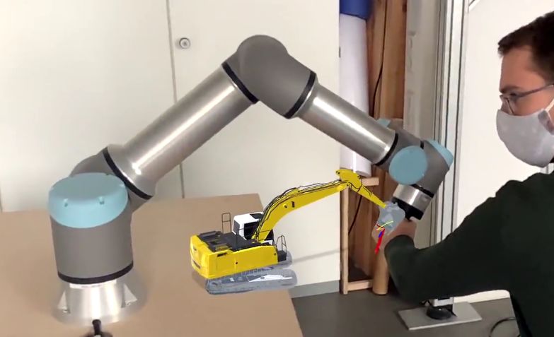
(a) Liebherr excavator (b) SCARA (4 joints) (c) Franka Emika
(4 joints). with prismatic joint. Panda (7 joints).
Fig. 4. Robot models used as PR during the evaluation. The joints are
numbered ascending from the base to the tip for each robot. Fig. 5. Recorded joint space trajectories of the excavator’s DT. The upper
and lower joint limits are drawn as dashed lines. The black line marks the
point in time when a velocity impulse is applied to joint 3.
Kinematics Dynamics Library (KDL) [16]. For the integration
of (8), the fourth-order Runge-Kutta method was used.
For the visual rendering of the DT and other information
such as forces and environmental information, the iviz
visualization platform [12] is deployed. By leveraging the
Unity Game Engine and a high-performance ROS interface,
iviz enables effortless robotic visualization on a variety
of AR/VR devices, including systems running Apple iOS,
Microsoft Windows, and Google Android. Due to the full
compatibility with ROS and the URDF-format, iviz requires Fig. 6. Joint space trajectories of the SCARA manipulator’s DT, when
singularities (q[2] = 0) are passed.
zero porting effort for existing ROS applications and has a ¯
function range that is comparable with the ROS-tool rviz.
A. Joint Limits
VI. E XPERIMENTAL R ESULTS
In order to test the behavior of the DT’s joint limits, the
For the evaluation, a Universal Robots UR16e manipulator, manipulator of an excavator as shown in Fig. 4(a) was used
which can be considered as a low-end haptic device, was as the PR. Therefore, the end effector of the DT, i.e., the
used as an HR. This choice was made to demonstrate that shovel, was moved around by hand to hit the joint limits on
the presented algorithms do not rely on the availability of purpose. The resulting joint space trajectories are depicted
special haptic interfaces. The Cartesian pose control of the in Fig. 5. Clearly, it can be seen that all joint limits are
UR16e was realized using the inverse kinematics algorithm respected without oscillations at the boundaries, independent
presented in [17]. The control loops were set to a frequency of the number of joints at the limit. At t = 14 s, joint 2 (boom)
of 500 Hz running on a laptop with an Intel Core i7-9570H reaches its lower limit causing a sudden change in the velocity
CPU. To demonstrate the capabilities of the proposed haptic of joint 3. This demonstrates that the impulse preservation
rendering method, a set of different PRs as depicted in Fig. 4 described in Section IV-B.3 works as expected. In general,
was selected. The chosen manipulators include a variety of the obtained joint trajectories are ready to be processed for
kinematic structures reaching from classical industrial to more validation or to be directly sent to the executing robot.
exotic manipulators. In addition, prismatic and revolute joints
are included as well as a redundant kinematic structure. B. Singularities
For all experiments, the friction parameters were chosen
empirically as djnt = 0.8 N m s, dcart,p = 17.0 N s m−1 , The SCARA arm from Fig. 4(b) features a singularity if
and dcart,θ = 1.5 N m s. The inertia values were set to it is stretched to its full extent (q[2] = 0). As illustrated in
mmain = 30.0 kg, Imain = 0.03 kg m2 , mother = 6.0 kg, and ¯
Fig. 6, this singularity neither restricts the movements of
Iother = 6.0 × 10⁻³ kg m2 . These values result in a user the remaining joints nor the proposed rendering algorithm
experience with reasonable required user forces without being in general. The manipulator can be moved into and out of
susceptible to force/torque sensor noise or exceeding the singularities at any time if suitable forces are applied as one
driving capabilities of the actuators. might expect from the real mechanical structure.Fig. 8. Iviz visualization of the programming process for an excavator. The
robot model is rendered in real-time onto the camera image of an Apple
iPad.
programming scenario, and the design of assistive features
Fig. 7. Translational and rotational tracking error between HR and DT for such as the display of forces due to collisions between the DT
different maximal forces and torques. The ∞-symbol in the legend indicates,
when the maximal forces and torques are not bounded.
and its environment. Additionally, the presented programming
approach will be evaluated with a group of test subjects.
C. Tracking Error At the theoretical level, the stability of the system during
human-robot interaction needs to be studied. Especially the
For the goal of accurate robot programming, it is crucial
observation, that a limited force input yields a bounded
that the HR closely follows the DT and vice versa. As
tracking error, which would imply stability, needs to be proven
explained in Section IV-C, the pose of the DT is used
mathematically.
as an input for the Cartesian controller of the HR. This
implies that the achievable tracking error depends on the R EFERENCES
controller properties of the HR. To examine the accuracy, [1] G. Biggs and B. MacDonald, “A survey of robot programming
the tracking errors for the translation pH H∗ and the rotation systems,” in Proceedings of the Australasian conference on robotics
H
θH∗ were evaluated for different maximal ¯ forces and torques and automation, 2003.
¯ [2] G. F. Rossano, C. Martinez, M. Hedelind, S. Murphy, and T. A.
exerted by the user, when the robot in Fig. 4(c) was moved Fuhlbrigge, “Easy robot programming concepts: An industrial perspec-
around randomly. The results depicted in Fig. 7 indicate that tive,” in 2013 IEEE International Conference on Automation Science
the expected errors are bound. From this, it also becomes and Engineering (CASE), 2013, pp. 1119–1126.
[3] V. Villani, F. Pini, F. Leali, C. Secchi, and C. Fantuzzi, “Survey
apparent that lower errors can be achieved by limiting the on human-robot interaction for robot programming in industrial
force/torque artificially without changing the HR or its control. applications,” IFAC-PapersOnLine, vol. 51, no. 11, pp. 66–71, 2018.
[4] N. Ladeveze, J. Y. Fourquet, B. Puel, and M. Taı̈x, “Haptic assembly
D. Integration with VR/AR and disassembly task assistance using interactive path planning,” in
2009 IEEE Virtual Reality Conference, 2009, pp. 19–25.
Due to the implementation as a ROS node, seamless [5] M. Fennel, A. Zea, and U. D. Hanebeck, “Haptic-guided path generation
interoperability with iviz is enabled. This was successfully for remote car-like vehicles,” IEEE Robotics and Automation Letters,
tested through the haptic rendering and visualization of 2021, to appear.
[6] P. Marayong, M. Li, A. M. Okamura, and G. D. Hager, “Spatial
the manipulators shown in Fig. 4. An example for the motion constraints: Theory and demonstrations for robot guidance
visualization, that was performed with the HTC Vive (VR), the using virtual fixtures,” in 2003 IEEE International Conference on
Apple iPad (AR) as well as the Microsoft Hololens (AR) can Robotics and Automation, vol. 2, 2003, pp. 1954–1959.
[7] N. Zafer, “Constraint-based haptic rendering of a parametric surface,”
be found in Fig. 8. We refer the reader to the supplementary Proceedings of the Institution of Mechanical Engineers, Part I: Journal
material of this paper for more examples.1 of Systems and Control Engineering, vol. 221, no. 3, pp. 507–517,
2007.
VII. C ONCLUSIONS [8] Z. Makhataeva and H. A. Varol, “Augmented reality for robotics: A
review,” Robotics, vol. 9, no. 2, 2020.
In this paper, a haptic rendering algorithm suitable for the [9] H. Fang, S. K. Ong, and A. Y. Nee, “Robot programming using
programming of serial manipulators was presented. Practical augmented reality,” in 2009 International Conference on CyberWorlds,
tests demonstrated that the presented rendering method 2009, pp. 13–20.
[10] A. Burghardt, D. Szybicki, P. Gierlak, K. Kurc, P. Pietruś, and R. Cygan,
provides a feasible solution for the joint space trajectories “Programming of industrial robots using virtual reality and digital twins,”
of the PR, independent of the presence of singularities or Applied Sciences, vol. 10, no. 2, 2020.
the kinematic structure. Furthermore, it was shown that the [11] D. Ni, A. W. W. Yew, S. K. Ong, and A. Y. C. Nee, “Haptic and
visual augmented reality interface for programming welding robots,”
achievable tracking accuracy mainly depends on the controller Advances in Manufacturing, vol. 5, no. 3, pp. 191–198, 2017.
of the HR and the magnitude of input force and torque. The [12] A. Zea and U. D. Hanebeck, “iviz: A ROS visualization app for mobile
overall system is well integrated with VR/AR methods. devices,” Software Impacts, vol. 8, 2021.
[13] D. Baraff, “Physically based modeling,” in SIGGRAPH 99 course notes,
Future research will involve the integration of an HR with 1999.
a faster Cartesian controller, the application in a real-world [14] R. Featherstone and D. E. Orin, “Dynamics,” in Springer Handbook
of Robotics, B. Siciliano and O. Khatib, Eds. Berlin, Heidelberg:
1 https://youtu.be/5t37cfeE7E0 Springer, 2008, pp. 35–65.[15] R. Featherstone, Robot dynamics algorithms. Boston, Dordrecht,
Lancester: Kluwer Academic Publishers, 1987.
[16] P. Soetens, T. Issaris, H. Bruyninckx, S. Joyeux, R. Smits et al. (2021,
Feb.) KDL overview – Orocos documentation. [Online]. Available:
https://docs.orocos.org/kdl/overview.html
[17] S. Scherzinger, A. Roennau, and R. Dillmann, “Inverse kinematics
with forward dynamics solvers for sampled motion tracking,” in 2019
19th International Conference on Advanced Robotics (ICAR), 2019,
pp. 681–687.You can also read