High Resolution Orthomosaics of African Coral Reefs: A Tool for Wide-Scale Benthic Monitoring
←
→
Page content transcription
If your browser does not render page correctly, please read the page content below
remote sensing
Article
High Resolution Orthomosaics of African Coral
Reefs: A Tool for Wide-Scale Benthic Monitoring
Marco Palma 1,†         , Monica Rivas Casado 2, *    , Ubaldo Pantaleo 1,3 and Carlo Cerrano 1
 1    Dipartimento di Scienze della Vita e dell’Ambiente (DISVA), Via Brecce Bianche, Monte Dago,
      60130 Ancona, Italy; m.palma@pm.univpm.it (M.P.); info@ubicasrl.com (U.P.); c.cerrano@univpm.it (C.C.)
 2    Cranfield Institute for Resilient Futures, School of Water, Energy and Environment, Cranfield University,
      Cranfield MK430AL, UK
 3    UBICA srl (Underwater BIo-CArtography), Via San Siro 6/1, 16124 Genova, Italy
 *    Correspondence: m.rivas-casado@cranfield.ac.uk; Tel.: +44-(0)-1234-750-111
 †    Cranfield Institute for Resilient Futures, School of Water, Energy and Environment, Cranfield University,
      Cranfield MK430AL, UK

 Academic Editors: Stuart Phinn and Xiaofeng Li
 Received: 27 March 2017; Accepted: 4 July 2017; Published: 8 July 2017

 Abstract: Coral reefs play a key role in coastal protection and habitat provision. They are also well
 known for their recreational value. Attempts to protect these ecosystems have not successfully
 stopped large-scale degradation. Significant efforts have been made by government and research
 organizations to ensure that coral reefs are monitored systematically to gain a deeper understanding
 of the causes, the effects and the extent of threats affecting coral reefs. However, further research is
 needed to fully understand the importance that sampling design has on coral reef characterization
 and assessment. This study examines the effect that sampling design has on the estimation of
 seascape metrics when coupling semi-autonomous underwater vehicles, structure-from-motion
 photogrammetry techniques and high resolution (0.4 cm) underwater imagery. For this purpose, we
 use FRAGSTATS v4 to estimate key seascape metrics that enable quantification of the area, density,
 edge, shape, contagion, interspersion and diversity of sessile organisms for a range of sampling scales
 (0.5 m × 0.5 m, 2 m × 2 m, 5 m × 5 m, 7 m × 7 m), quadrat densities (from 1–100 quadrats) and
 sampling strategies (nested vs. random) within a 1655 m2 case study area in Ponta do Ouro Partial
 Marine Reserve (Mozambique). Results show that the benthic community is rather disaggregated
 within a rocky matrix; the embedded patches frequently have a small size and a regular shape;
 and the population is highly represented by soft corals. The genus Acropora is the more frequent
 and shows bigger colonies in the group of hard corals. Each of the seascape metrics has specific
 requirements of the sampling scale and quadrat density for robust estimation. Overall, the majority
 of the metrics were accurately identified by sampling scales equal to or coarser than 5 m × 5 m and
 quadrat densities equal to or larger than 30. The study indicates that special attention needs to be
 dedicated to the design of coral reef monitoring programmes, with decisions being based on the
 seascape metrics and statistics being determined. The results presented here are representative of
 the eastern South Africa coral reefs and are expected to be transferable to coral reefs with similar
 characteristics. The work presented here is limited to one study site and further research is required
 to confirm the findings.

 Keywords: seascape metrics; structure-from-motion; FRAGSTATS; photogrammetry; sampling scale;
 quadrat density; sampling strategy; sampling framework

Remote Sens. 2017, 7, 705; doi:10.3390/rs9070705                           www.mdpi.com/journal/remotesensing
Remote Sens. 2017, 7, 705                                                                             2 of 26

1. Introduction
      Coral reefs provide key provisioning, cultural and regulating ecosystem services [1,2]. Their economic
value has been estimated in recent studies through the ecosystem services theory developed by
Samonte et al. [3], Seenprachawong [4] and the Millennium Ecosystem Assessment’s classification [5].
Within the context of provisioning and cultural services, coral reefs provide an important protein
source and a basin for livelihoods for fisheries in addition to scenic beauty for recreational tourism [6].
Regarding regulating services, coral reefs provide coastal protection by dissipating the waves energy [7]
and contribute to the regulation of the coastal line erosion and sedimentation [6]. The benefits of coral
reefs are therefore vast and varied. However, anthropogenic threats at the regional and global scale
have considerably impacted coral reefs, with 19% of reefs considered completely lost and 60–75%
of reefs threatened by 2011 [8–10]. The increase of extreme weather events impacting the coast [11]
has also played a significant role in large-scale degradation. As a result, coral reef protection has
become a priority in many governmental agendas (e.g., [12]). This has resulted in the development
and implementation of scientific surveys and monitoring programs aimed at evaluating the causes,
effects and extent of coral threats (e.g., sedimentation, bleaching and climate change) [13–15].
      In general, wide-area (>1500 m2 ) coral reef monitoring methods are based on remote sensing
approaches that range from autonomous or semi-autonomous underwater vehicles [13,16–19] to
satellite and airborne imagery [20–23]. For the particular case of wide-area (>1500 m2 ) in situ
monitoring, the key limitations are cost, access to the site and the spatio-temporal extent to be covered
[15]. In situ refers hereinafter to all techniques that require human presence at the site to obtain relevant
samples (e.g., photographs or biological samples), and its meaning is specific to this manuscript. In situ
methodologies provide higher spatial resolution than wide-area (>1500 m2 ) remote sensing methods
(e.g., satellites) and are essential for the understanding of very fine ecological processes [15,24].
New technologies and analytical solutions (e.g., autonomous and semi-autonomous underwater
vehicles, boat-based systems and close range Structure-from-Motion (SfM)) have been developed
and can help fulfil the need for wide-area (>1500 m2 ) high resolution data provision [13,18,19,25,26].
This scientific advance in coral reef monitoring relies on the integration of low cost off-the-shelf cameras
and state of the art photogrammetric techniques (i.e., SfM) [27,28]. The resulting data products include
high resolution (finer than 5 cm) Digital Elevation Models (DEMs), point clouds and two-dimensional
mosaics [19,29,30], which enable the 2D and 3D analysis of coral reef ecological processes at different
scales through the use of key metrics [19,25–27,31,32]. Examples of the use of these techniques include
Burn [33], Chirayath [34], Gutierrez [35] and Lavy [36]. Burns [33] used 3D SfM-derived models to
estimate key metrics that informed on changes to the benthic habitat along 25 m long transects and
covering around 250 m2 . Chirayath [34] applied SfM techniques to map a 15 km2 coral reef area in the
Shark Bay (Australia) and to generate an accurate bathymetric map from an unmanned aerial vehicle.
Gutierrez [35] applied SfM to generate 3D models of the benthic organisms for taxonomic identification
purposes, whereas Lavy [36] applied SfM techniques to derive morphological measurement of corals.
      Several authors have looked at the application of seascape ecology metrics to characterize the
ecological processes of coral reefs [37,38]. However, little effort has yet been made to define the
appropriate sampling strategy to accurately determine each of the metrics; the ecological rational for
scale selection is usually unsupported [37]. Generally, scale selection is based on arbitrary choices
or convention, albeit scale having an impact on seascape metric estimation [39]. The importance of
standardized sampling protocols has already been recognized by several authors [37]. For example,
Lecours et al. [24] recognizes the need for multiple scale approaches in benthic habitat mapping and
states that sampling should be planned in order to describe those variables relevant for the study.
Boström et al. [37] recognizes the design of a survey as a key future research priority for seascape
ecology; the wide range of spatio-temporal scales used in seascape studies inhibits the ability to directly
compare studies’ outcomes, identify general patterns, predict consequences across systems and design
coastal reserves based on relevant information. Kendall and Miller [39] underline the negative effects
of changes in map resolution when representing ecological landscape indexes. Garrabou et al. [40,41]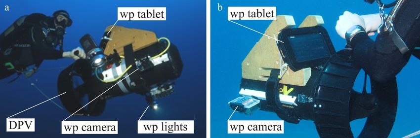
Remote Sens. 2017, 7, 705                                                                            3 of 26

proposed the calculation of landscape metrics at centimeter resolution in accord with the principles of
landscape ecology [42].
      There are multiple studies that [20,43–45] investigate the effect that the sampling design (i.e., the
combined effect of scale, quadrat density and sampling strategy) has on metric estimation. For example,
Costa et al. [20] carried out a comparative assessment for bathymetry and intensity characterization at
two different spatial scales (4 m × 5000 m and 4 m × 500 m), whereas Pittman et al. [43] quantified
seven different morphometrics at multiple scales (i.e., 15 m, 25 m, 50 m, 100 m, 200 m, 300 m radius)
from a 4 m bathymetry grid. Both studies showed that the spatial scale had an influence on the derived
metrics. Wedding et al. [44] used a stratified sampling strategy to estimate rugosity and compare it to
rugosity estimates obtained from a DEM at four grid sizes (i.e., 4 cm, 10 cm, 15 cm and 25 cm). Results
showed that the 4 m grid was the only grid size showing a significant positive association with the in
situ rugosity. The author proposed the method as non-substitutive of the finer scale rugosity methods
for characterizing coral reef communities, but as an effective alternative for broad scale assessments.
Purkis et al. [45] used a kernel radius of 4 m, 8 m, 20 m and 40 m with an increment of 20 m–400 m
to estimate rugosity and habitat. In their study, results indicated that the habitat of up to (but likely
not exceeding) 40 m away, most strongly influenced the diversity and particularly the abundance of
certain fish guilds.
      Here, multiple sample scales and quadrat densities applied on a high resolution (1.8 cm) wide
area (>1500 m2 ) dataset, where sample scale indicates the sampling quadrat size and quadrat density
refers to the number of quadrats taken within a target area, will be compared. The aim of the
study is to develop an SfM-based monitoring framework for the estimation of seascape metrics using
semi-autonomous vehicles with embedded cameras for imagery collection for the case of the study area
of Ponta do Ouro, Mozambique. This will be achieved through the following overarching objectives:

  (1) to quantify the trade-offs between sample scale and robustness in seascape metric estimation;
  (2) to quantify the trade-offs between sample quadrat density and robustness in seascape
      metrics estimation;
  (3) to define a set of guidelines for seascape metric estimation based on findings from (1) and (2).

2. Material and Methods

2.1. Study Site
     The study area is located in the Partial Marine Reserve of Ponta do Ouro, Mozambique (Figure 1a)
and is part of the Isimangaliso Wetland Park, which protects the southernmost tropical coral reefs of
the African continent [46]. The coral reef system is dominated by non-accretive corals running parallel
to the coastline at 1–2 km from the shore [47,48]. Outcrops are present (Figure 1b,c) and originate from
fossilization of Late Pleistocene beaches and dunes [49] that form very flat structures [50]. The area is
characterized by high levels of endemic species [51–53] with the coral cover being dominated by soft
corals that are tolerant to strong wave energy and sediment resuspension [54–57].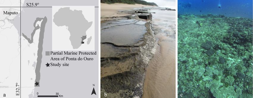
Remote Sens. 2017, 7, 705                                                                                4 of 26

      Figure 1. (a) Location of the study site in the Partial Marine Protected Area of Ponta do Ouro
      (Mozambique); (b) detailed image showing the fossils dune outcrops along the sandy littoral;
      (c) detailed image showing the submerged outcrops at the dive site.

2.2. Data Acquisition
    Data collection was carried out by two SCUBA divers using a Sierra Dive Xtras (Xtras, Ltd.,
Mukilteo, WA, USA) Diver Propulsion Vehicle (DPV) equipped with a GoPro Hero3 Silver (Woodman
Labs, Inc., San Mateo, CA, USA) and an Asus Google Nexus 7 tablet (Google Inc., Mountain View,
CA, USA) embedded within an Alltab dry case system (Alleco Ltd., Helsinki, Finland) (Figure 2).
The camera was set to time-lapse mode, recording nadir images at 1 Hz frequency with a focal length
equivalent to 21 mm. Inertial navigation data obtained from the gyroscope and the accelerometer were
logged via an Ubica Underwater Position System (UUPS) [58] be-spoke application. The logged data
were then used to derived camera pitch, yaw and roll.

      Figure 2. (a) A general photograph of the Diver Propulsion Vehicle (DPV) equipped with the Hero3
      Silver camera, the waterproof tablet and the lights; (b) detailed image of the waterproof camera and
      tablet. “wp” stands for waterproof.

     The sampling path was defined by two 50 m ancillary tapes distributed following homogeneous
seascape characteristics identified in a pre-deployment survey (Figure 1c). The exact path followed
by the diver was recorded via a towed buoy with an integrated Etrex10 GPS (Garmin Ltd., Lenexa,
KS, USA). The GPS coordinates were recorded in Wide Area Augmentation System (WAAS) mode
at 1 Hz frequency and projected into the Universal Transverse Mercator (UTM) fuse 36 Southern
Hemisphere coordinate system, defined by the World Geodetic System (WGS84), within a Geographical
Information System (GIS) environment (ArcGIS 10.1, Redlands, CA, USA). The diver maintained an
average swimming speed of 0.75 m s−1 and an average distance to the sea bottom of 2.7 m, with the
range being between 1.5 m and 3 m and with each frame covering 3 m2 (Figure 3a).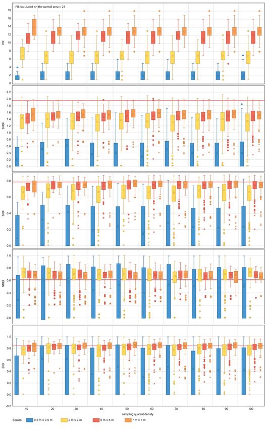
Remote Sens. 2017, 7, 705                                                                                     5 of 26

      Figure 3. Schematic workflow overview for the field data collection and data analysis implemented:
      (a) transect deployment and image collection (left) and detailed example of the collected imagery
      (right); (b) processed orthoimage of the transects with the example of nested quadrats (left) and the
      detail of the nested sampling scales applied (right); (c) digitized output showing the abundance of
      different classes of benthic organisms; (d) summary of sampling scale, quadrat density and strategy
      applied; (e) graphical example of the digitized sessile organisms within different sampling scales. * and
      ** refer to the classification proposed by Edinger and Risk [60] and the classes used by Schleyer and
      Celliers [49], respectively. ID stands for Identification Code.

     Consecutive frames were taken with an approximate overlap of 70% along and 45% across the
path. The sampling was performed in the central area of the reef covering a total of 1655 m2 at an
average depth of −22 m AMSL. All datasets were acquired on the 8 May 2015 during one single dive
with a SCUBA dive. Data were collected during steady and calm sea-weather condition with good
visibility (estimated 20 m) and avoiding the lowest and the highest tides.
     All the underwater imagery was collected within 15 min. A total of four hours was required to set
up the equipment on site (e.g., mount the camera, deploy the tape underwater, set up the parameters,
implement the field briefing). An additional hour was required after the dive to check that all the
imagery had been captured correctly and the UUPS had logged all of the required information. An
extra 20 min were required to pack the equipment.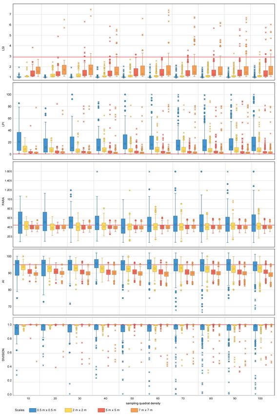
Remote Sens. 2017, 7, 705                                                                           6 of 26

2.3. Photogrammetric Process and Digitization
       A total of 1192 images collected were visually inspected, and only those with the right
characteristics (i.e., 3200 × 2400 pixel high image quality and consecutive spatial coverage) were
considered for further analysis (Figure 3a). A total of 8 h were required to visually inspect all the
frames acquired. From the initial set of images, 1182 were included in the photogrammetry process. All
the frames were captured at 1 cm resolution with a final orthoimage resolution of 1.8 cm. The metadata
of each JPEG were stored in Exchangeable Image File format (EXIF) along with other camera parameters
(e.g., camera model and optical lens characteristics) and directly loaded into Photoscan (Agisoft LLC.,
St. Petersburg, Russia). The exact position of each frame centroid was estimated by coupling the
camera recording time with the GPS watch based on Roelfsema et al. [59]. pixGPS (BR Software,
Asker, Norway) was used for that purpose. The coordinates for each of the frames were used to
georeference (scale, translate and rotate) the imagery into the coordinate system defined by the World
Geodetic System (WGS84) and to minimize geometric distortions. Image coregistration errors were
automatically estimated by Photoscan as the difference between the positions measured through GPS
and the coordinates derived from the imagery. The overall process to obtain the orthoimage took 12 h
of processing time based on the performance of an Asus laptop (Beitou District, Taipei, Taiwan) with
an Intel Core i7-3630QM 2.40-GHz processor (Intel Corporation, Santa Clara, CA, USA), 16 Gb RAM
and graphic card NVIDIA Geoforce GTX 670M (NVIDIA Corporation, Santa Clara, CA, USA).
       Mega-epibenthic sessile organisms (i.e., seabed living organisms with a body diameter of 5 cm
approximately) were manually identified and digitized to the finest possible taxonomic level and
then clustered according with common morphological characteristics following the approach by
Edinger and Risk [60] and the descriptions published by Schleyer and Celliers [49]. The morphological
classification also accounted for non-coral organisms, such as sponges and other sessile invertebrates
(i.e., tunicates and ascidians). The orthoimage was digitized manually and classified within ArcGIS
(Figures 3b,c and 4a,b). The background rocky substrate, within which patches were embedded as
“islands”, was considered as the seascape matrix (i.e., rocky matrix) following the island biogeography
theory proposed by MacArthur and Wilson [61]. The digitization process required 21 days (i.e., 147 h
at 7 h per day). A total of 7547 individual organisms were digitized from the orthoimage.

2.4. Seascape Metric Estimation
     Seascape metrics were estimated from the orthoimage for a set of different sampling designs
described by all the possible combinations of a range of sampling scales, quadrat densities and
sampling strategies. Within the scope of this study, the sampling scale refers to the size of the sampling
quadrats and ranged from 0.5 m × 0.5 m–7 m × 7 m (Figure 3d); the quadrat density is the number of
quadrats taken within the target area and ranged from 10–100 in consecutive increments of 10 quadrats;
and the sampling strategy refers to the spatial distribution of the samples (i.e., nested or random)
(Figure 3e). The sampling designs were overlaid onto the orthoimage within ArcGIS.
     Nested sampling approaches require the overlap of quadrat centroids of consecutively increasing
scales. Each scale appears only once in each set of overlapped centroids, with each set being randomly
distributed across the reef. The range of values considered for the sampling scale, quadrat density and
sampling strategy was selected based on the size of the sessile organisms, their spatial distribution, the
magnitude of the effects to be measured and standard sampling protocols for coral reefs [19,62–64]. A
total of three replications were obtained for each combination of sample scale, quadrat density and
sampling strategy to account for spatial variability. All quadrats were inspected to ensure that at
least 60% of their surface fell within the extent of the coral reef area. Although the centroid of the
quadrat was always forced to be within the surveyed area, this did not guarantee that all the quadrat
fell within the boundary. Those quadrats with more than 40% of their surface falling outside the
coral reef boundaries were excluded from the analysis. The spatial distribution of sampling quadrats
was automated in ArcGIS using a range of tools (i.e., create random points, buffer, envelope feature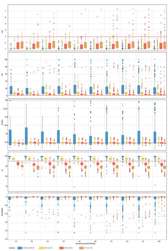
Remote Sens. 2017, 7, 705                                                                               7 of 26

to polygon, iterate feature classes, clip, invert, merge and polygon to raster) within the ArcMAP
model builder.
     Seascape metrics were derived using FRAGSTATS v4 (Amherst, MA, USA) [65], a software
developed to compute a wide variety of landscape metrics for categorical map patterns that has
successfully been applied for seascape ecology [38–40,66]. Only metrics that could be automatically
derived from FRAGSTATS were considered within this study because of their potential to enhance the
autonomy of the framework. From the more traditional metrics used for coral reef characterization,
only cover was calculated, as it is a key metric used to assess the benthic community composition.
     FRAGSTATS estimates key landscape metrics, hereinafter referred to as seascape metrics, based
on the disposition of the patches within the landscape (i.e., seascape). Here, a patch is each of
the digitized individual polygons (Figure 4). A set of metrics defining area-density-edge, shape,
contagion and interspersion, as well as diversity was selected based on their relevance to seascape
ecology composition (Table 1).

      Figure 4. (a) The processed orthoimage; (b) the map of the digitized benthic organisms; (c) the
      configuration of the digitized sessile organism within the case study area of Ponta do Ouro Partial
      Marine Reserve (Mozambique). * and ** refer to the classification proposed by Edinger and Risk [60]
      and the classes used by Schleyer and Celliers [49], respectively.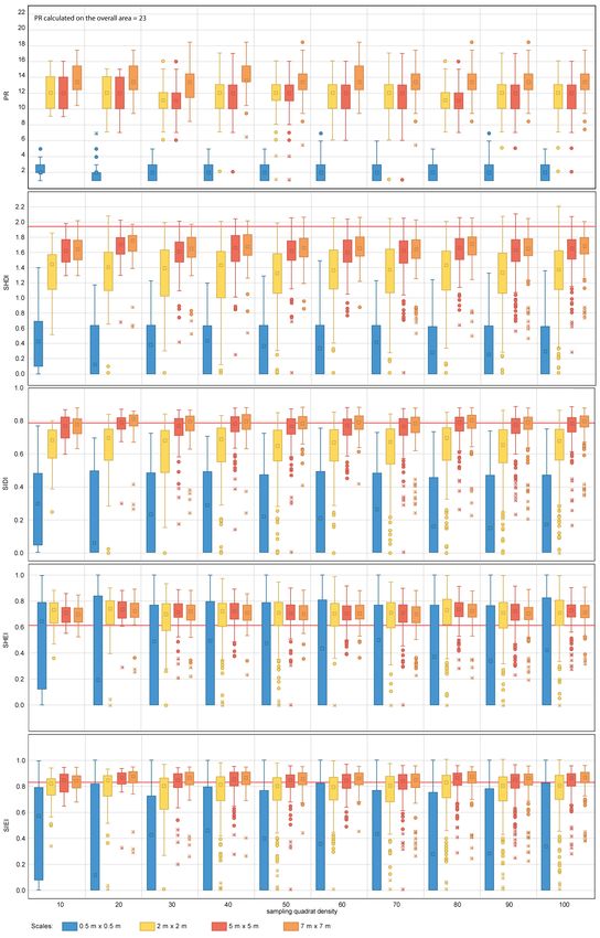
Remote Sens. 2017, 7, 705                                                                          8 of 26

      Area-density-edge metrics relate to the number and size of sessile organisms and the amount of
edges created by them. Here, the edge is the border between adjacent patches. This group of metrics
includes the Landscape Shape Index (LSI) and the Largest Patch Index (LPI) [65]. LSI informs about
the morphological aggregation of the patches within a standardized seascape square. The value of LSI
increases without limit from 1 upwards as the seascape becomes disaggregated, where 1 represents
minimum disaggregation. LPI informs about the clumpiness of the seascape as the percentage value
within a standardized seascape square. It is a measure of patch dominance; LPI values of 100% indicate
that the seascape unit is dominated by a single patch. Both LSI and LPI provide information on the
composition of the sessile organism communities in size per class and on the structure of the reef;
seascapes that are highly subdivided into small patches are characteristics of low colonized substrates
where colonies have difficulties settling and cannot reach typical dimensions. This can be caused by
multiple factors, such as sediment resuspension and deposition or high wave energy [57].
      Shape metrics (i.e., Perimeter Area Ratio (PARA) change) [65,67] are directly estimated from the
shape of the organisms. In particular, PARA estimates the ratio between the perimeter and the area
of all the patches within the seascape unit and provides information on the shape complexity of the
patches in the seascape; an increase in the size of the patch results in a decrease in the value of PARA.
PARA is always larger than 0 and does not have an upper limit. The PARA value could be interpreted
as a good indicator of the growth conditions of corals; corals show constant radial allometric growth
[68], but this can be affected by external factors, such as intra-specific and inter-specific competition
and hydrodynamic conditions. Under affected allometric growth conditions, larger PARA values are
to be expected.
      Contagion and dispersion metrics (i.e., Aggregation Index (AI) and Division index
(DIVISION)) [65] look at the seascape texture by examining the aggregation and intermix of the
class of organisms. AI [65,69] quantifies the adjacencies per patch type within the seascape and informs
on the homogeneity of the composition of the benthic communities. It ranges from 0% (maximum
patch disaggregation) to 100% (maximum patch aggregation). High values of AI indicate that the
classes of patches are more clustered within the landscape. This could inform about the reproductive
biology of the species considered and the population dynamics; species with short larval dispersion
tend to create clusters of individuals near the organism. These species are more sensitive to local
extinctions [70]. Instead, DIVISION measures the heterogeneity of the seascape and estimates the
variability in patch types within the seascape. DIVISION ranges from 0–1, where a 0 value indicates
maximum aggregation, and values close to 1 indicate maximum disaggregation. These indexes provide
information on the composition of the coral and the planar morphology of the colonies within the
seascape; heterogeneous seascapes are composed by a varied benthic community or placed at the edge
of the reef, where just a few individuals per specie are settled.
      Diversity metrics focus on the number of organisms and their distribution within the seascape.
They are an indication of the resilience of the coral reef and its ability to withstand significant
disturbances [71]. Within this group, five key metrics have been estimated: Patch Richness (PR),
Shannon’s Diversity Index (SHDI), Simpson’s Diversity Index (SIDI), Shannon’s Evenness Index (SHEI)
and Simpson’s Evenness Index (SIEI) [65]. PR informs about the number of patches present within the
seascape. SHDI [72] informs about the number of different patch types within the seascape and how
evenly these types are distributed. SHDI can present any positive value from 0 upwards. Larger SHDI
values represent greater evenness amongst patch types within the seascape. SIDI [73] informs about the
probability that two entities (i.e., pixels) taken at random from the same seascape belong to different
patch types and ranges between 0 and 1. Larger SIDI values indicate a greater probability that two
pixels are from different patch types. Both SHEI and SIEI estimate the proportion of the maximum
Shannon’s or Simpson’s diversity index, respectively. SHEI and SIEI range from 0–1, where 1 indicates
that the area is distributed evenly among patch types.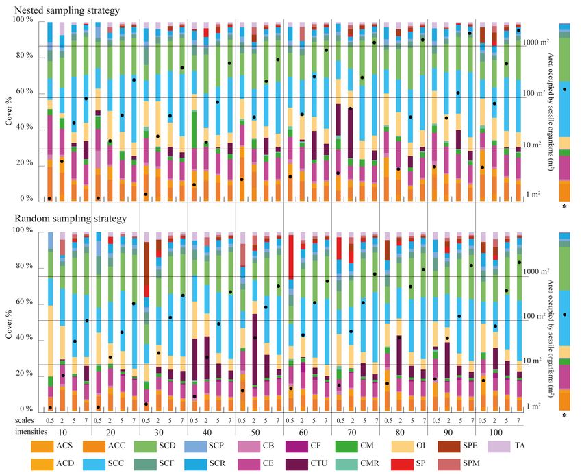
Remote Sens. 2017, 7, 705                                                                                                     9 of 26

      Table 1. Seascape metrics estimated for the case study area of Ponta do Ouro Marine Reserve
      (Mozambique). The seascape metric descriptions are based on those for landscape analysis obtained from
      FRAGSTATS v4 [65]. All metrics are dimensionless except for the Largest Patch Index (LPI) (%), AI (%)
      and DIVISION (ratio). Here, patch refers to each of the digitized individual polygons falling within a
      given morphological class.

      Metrics                   Index                    Description
                                                         Normalized ratio of edge (i.e., patch perimeters) to area
                                                         (i.e., seascape defined by the sampling scale) in which the total
                                                         length of edge is compared to a seascape with a standard
                                Landscape Shape          shape (square) of the same size and without any internal edge.
                                Index (LSI)              LSI = 1 when the seascape consists of a single square patch;
                                                         LSI increases without limit as the morphology becomes more
      Area Density Edge
                                                         disaggregated. LSI provides a simple measure of morphological
                                                         aggregation or clumpiness.
                                                         Percentage of the seascape comprised of the single largest patch.
                                Largest Patch            LPI approaches 0 when the largest patch is increasingly small.
                                Index (LPI)              LPI = 100 when the entire seascape consists of a single patch;
                                                         that is, when the largest patch comprises 100% of the seascape.
                                                         Simple ratio of patch perimeter to area in which patch shape
                                                         is confounded with patch size.
                                Perimeter Area
      Shape                                              The ratio is not standardized to a simple Euclidean shape
                                Ratio (PARA)
                                                         (e.g., square); an increase in patch size will cause a decrease in
                                                         the perimeter-area ratio.
                                                         The ratio of the observed number of like adjacencies to the
                                                         maximum possible number of like adjacencies given the
                                                         proportion of the seascape comprised of each patch type (%).
                                Aggregation Index (AI)
                                                         The maximum number of like adjacencies is achieved when the
                                                         morphological class is clumped into a single compact patch,
      Contagion Interspersion                            which does not have to be a square.
                                                         The probability that two randomly chosen pixels in the sea-
                                Division Index           scape are not situated in the same patch.Maximum values
                                (DIVISION)               are achieved when the seascape is maximally subdivided;
                                                         that is, when every pixel is a separate patch.
                                Patch Richness (PR)      Number of patch types present in the seascape.
                                                         Represent the amount of “information” per morphological class;
                                Shannon’s Diversity
                                                         larger values indicate a greater number of patch types and /or
                                Index (SHDI)
                                                         greater evenness among types.
                                                         The probability that any two pixels selected at random would
                                Simpson’s Diversity      correspond to different patch types; the larger the values
                                Index (SIDI)             the greater the likelihood than any two randomly drawn pixels
                                                         would be different patch types.
      Diversity                                          Proportion of maximum Shannon’s Diversity Index based
                                                         on the distribution of area among patch types and typically
                                Shannon’s Evenness
                                                         given as the observed level diversity divided by the
                                Index (SHEI)
                                                         maximum possible diversity given the patch richness.
                                                         SHEI = 1 when the area is distributed evenly among patch types.
                                                         Proportion of maximum Simpson’s Diversity Index based on the
                                                         distribution of area among patch types and typically given as
                                Simpson’s Evenness
                                                         the observed level diversity divided by the maximum possible
                                Index (SIEI)
                                                         diversity given the patch richness. SIEI = 1 when the area
                                                         is distributed evenly among patch types.

2.5. Data Analysis
     Composition and abundance for the full extent of the mapped coral reef area were estimated
based on the digitized sessile organism classes (Figures 3c and 4). The minimum and maximum
cover of individual sessile organisms (total surface in m2 ) identified within each quadrat for each
morphological class [49,60] were estimated. The average dimension, as well as the total count of
individuals within each morphological class were also reported. Robustness in metric estimation was
assessed for each sampling design based on the difference between the metric value estimated for a
specific sampling design and (i) that obtained for the whole surveyed area or (ii) that obtained for the
Remote Sens. 2017, 7, 705 10 of 26
most comprehensive sampling design considered (i.e., 7 m × 7 m and 100 quadrats). The effect on both
measures of central tendency (e.g., mean, median) and dispersion (e.g., range, standard deviation) was
assessed. Descriptive statistics and box-plots were used for that purpose. General trend patterns were
derived from these observations and used to compile a set of general guidelines for coral reef sampling.
3. Results
The line transect defined by the metric tape accounted for 650 m. The coregistration error of the
generated orthoimage was 4.08 m and 6.8 m for the x and y axis, respectively. Within the whole mapped
area (1655 m2 ), the benthic organisms covered 335.54 m2 , which equates to a total cover of 20.27%.
The coral reef was dominated by soft (Alcyonacea, 62.1% of the total cover) and hard corals
(Scleractinia, 31.00% of the total cover) (Figure 5). Within the soft corals, the dominant morphological
classes were (i) Soft Crested Coral (SCC) (soft corals that are rigid with mounted parallel lobes and
low in profile) and (ii) Soft Corals with Digitate lobules (SCD). These groups presented the largest
individual organism cover values (7 m2 ) and were represented by the genera Lobophytum, Sinularia
and Sarcophyton (Table 2). Hard corals were mainly represented by the genus Acropora (44.32% of the
total hard colony community). The more frequent class in the group was Acropora with digitated and
stubby branches (ACD), presenting also the largest surface dimensions (Table 2).
Non-Acropora Massive or Multilobate Corals (CM) include Platygyra spp., Montastrea spp.,
Galaxea spp., Favites spp., Favia spp. and Turbinaria sp.. The average size for this morphological
class was 0.019 m2 . In addition to the above groups, 141 colonies of free-living fungiid corals
were identified. These showed an average dimension of 0.006129 m2 (Table 2) and also included
11 encrusting and dome-shaped sponges. The Other Invertebrates (OI) presented the largest variance
in surface dimension with the tunicate Atriolum robustum, accounting for 0.0008 m2 , and the actinias
Stichodactyla spp., accounting for 1.04 m2 . The background rocky substrate accounted for 1150.55 m2 of
the total area (69.52%). The 10.27% (168.84 m2 ) of the overall coral reef area sampled, where individual
organisms could not be identified, was not digitized.
The exclusion of quadrats with more than 40% of the area falling outside the coral reef boundary or
presenting non-textured classes did not influence the overall analysis; the number of samples available
was large enough for the robust estimation of the descriptive statistics, boxplots and associated metrics
of species abundance and composition (Table 3).
The effect of scale, quadrant density and sampling strategy on cover estimation is summarized in
Figure 5. Sampling scales coarser than 5 m × 5 m provide similar cover estimates to those obtained for
the overall surveyed area, with the finest scale (0.5 m × 0.5 m) failing to accurately represent cover
estimates. This pattern is more noticeable for random sampling strategies than for nested strategies.
Regarding the quadrat density applied, no particular patterns can be observed as the number of
quadrats used in the survey is increased. However, sampling designs where the combined area
surveyed by the quadrats contains in excess of 100 m2 of benthic organisms closely resembles the cover
distributions observed within the whole surveyed area.Remote Sens. 2017, 7, 705 11 of 26
Figure 5. Percentage of cover per morphological class for each sampling design considered in the study.
The proportion is estimated as the ratio between the area occupied by each morphological class over
the total area covered by the sessile organisms within each sampling design. The values presented refer
to the average cover of the three replicates taken within each sampling design. The “*” indicates the
total area covered by the sessile organisms in each sampling design estimated as the average of the
three replicates taken. The last column shows the cover per morphological class for the totality of the
coral reef surveyed.
For area-density-edge metrics, the overall area surveyed scores an LSI value of 2.91 (Table 4).
The LPI value for the sampled coral reef is 0.47% (Table 4). The LSI values for independent quadrats
range between one and eight, showing that there is spatial heterogeneity in aggregation across the coral
reef. The dispersion of LPI values obtained within some of the sampling design tested is large, with
LPI values ranging from 0%–100% in some cases. For both LSI and LPI, the sampling quadrat density
has a larger impact on the estimation of the measures of dispersion (e.g., range, standard deviation)
than on the estimation of measures of central tendency (e.g., mean, median). For LSI, quadrat densities
above 70 are required to characterize the measures of dispersion for nested strategies to the same
level as the most comprehensive quadrat density applied (i.e., 100), whereas quadrat densities above
40 are required for random strategies. For LPI, quadrat densities above 40 and 30 are required to
characterize the measures of dispersion for nested and random strategies, respectively. In contrast,
the sampling scale has a larger impact on the measures of central tendency than on the measures of
dispersion. The finest scale (0.5 m × 0.5 m) presents the largest deviations from the seascape metrics
obtained for the overall coral reef area. For LPI, sampling scales of 5 m × 5 m and 7 m × 7 m provided
good approximations to the metrics obtained for the totality of the coral reef area for both nested and
random strategies (Figures 6 and 7). However, for LSI, coarse scales (7 m × 7 m) were required for
both nested and random strategies.Remote Sens. 2017, 7, 705 12 of 26
Table 2. Description of the key morphological classes of benthic organisms and their count, maximum
(max), minimum (min) and average dimensions (m2 ), identified within the coral reef studied in the
Partial Marine Reserve of Ponta do Ouro (Mozambique).
Average Max Min
Acronym Description Count
Dimension Dimension Dimension
ACB Acropora, branching (e.g., A. austera) 15 0.384 ± 0.016 0.716 0.225
ACD Acropora, digitate, stubby (e.g., A. humilis) 465 0.069 ± 0.010 0.821 0.044
Acropora, columns and blades, very stout
ACS 109 0.054 ± 0.068 0.467 0.001
(e.g., A. palifera and A. cuneata)
ACC Acropora, stout branches, low bushy shape 20 0.045 ± 0.041 0.148 0.005
Non-Acropora massive or multilobate
CM corals (e.g., Platygyra spp. 559 0.019 ± 0.038 0.544 0.0005
and Galaxea spp.)
Low relief, often small colonies
CE 533 0.083 ± 0.112 1.281 0.002
(e.g. Porites spp.)
CTU Tabular coral (e.g., Turbinaria sp.) 4 0.300 ± 0.573 1.160 0.009
CMR Free-living fungiid corals 141 0.006 ± 0.004 0.034 0.015
Branching non-Acropora corals
CB 275 0.011 ± 0.012 0.089 0.065
(e.g., Pocillopora spp.)
Foliose, either horizontal or vertical,
CF non-Acropora, (e.g., Montipora spp., 2 0.065 ± 0.069 0.1138 0.0164
Echinopora spp.)
Other invertebrates inclusive of
OI gasterops, tunicates, echinoderms 339 0.067 ± 0.134 1.044 0.00008
and other hexacorals
Erect in profile, but soft and
SCF pliable with an expanded disk 461 0.023 ± 0.021 0.137 0.046
and stalk (e.g., Sarcophyton spp.)
Soft and pliable colonies
SCD 1916 0.042 ± 0.205 7.6134 0.045
(e.g., Sinularia spp.)
Low in profile and rigid with
SCC 1721 0.061 ± 0.197 4.376 0.645
mounded radial (e.g., L. latilobatum)
Low in profile and rigid with
SCR erect radial or parallel lobes 342 0.032 ± 0.068 0.974 0.002
(e.g., L. crassum).
Low in profile and plane on the
SCP 466 0.009 ± 0.007 0.0562 0.0007
surface (e.g., L. depressum)
SP General sponges 6 0.041 ± 0.031 0.092 0.001
SPM Massive or dome-like sponges 3 0.075 ± 0.038 0.119 0.046
SPE Encrusting sponges 2 0.070 ± 0.022 0.086 0.055
TA Algae and algal turf 168 0.010 ± 0.018 0.144 0.0004
The PARA shape metric (Figures 6 and 7) reaches values of 4.5 × 10⁵ (Table 4) for the whole area
surveyed. The multiple sampling scales considered report different results in terms of measures of
dispersion. Scales finer than 2 m × 2 m report dispersion values considerably larger than coarser
scales and are characterized by PARA metric overestimation. The pattern is more prominent for
nested strategies, where PARA values of individual quadrats reach magnitudes of 3 × 10⁶ , whereas for
random strategies, the maximum values do not exceed magnitudes of 1.6 × 10⁶ . The quadrat density
also influences the estimation of the measures of dispersion, with the range of PARA decreasing as the
number of quadrats increases for both nested and random sampling strategies. Quadrat densities of 40
and 30 provide similar results to those obtained for the maximum quadrat densities applied (i.e., 100)
for nested and random strategies, respectively.Remote Sens. 2017, 7, 705 13 of 26
Table 3. Sample size per combination of sampling scale, quadrat density and strategy considered, after
exclusion of non-valid samples (i.e., quadrats with more than 40% of the area falling outside the coral
reef boundary or presenting non-textured morphological class).
Scale 0.5 m × 0.5 m 2m×2m 5m×5m 7m×7m
Expected
Density Random Nested Random Nested Random Nested Random Nested
10 24 25 29 28 28 28 27 27 30
20 50 49 54 56 53 53 44 44 60
30 73 70 78 83 80 80 73 73 90
40 91 98 113 116 108 108 109 109 120
50 127 117 142 142 136 136 130 130 150
60 145 146 178 176 167 167 161 162 180
70 164 161 201 204 202 202 190 190 210
80 191 187 237 234 225 225 223 223 240
90 213 216 260 265 244 245 250 250 270
100 240 239 287 290 291 290 270 282 300
Table 4. Seascape metric values obtained for the total coral reef area surveyed. The metrics reported
include: Landscape Shape Index (LSI), Large Patch Index (LPI), Perimeter Area Ratio (PARA),
Aggregation Index (AI), Division Index (DIVISION), Patch Richness (PR), Shannon’s Diversity Index
(SHDI), Simpson’s Diversity Index (SIDI), Shannon’s Evenness Index (SHEI) and Simpson’s Evenness
Index (SIEI).
Acronym Value Acronym Value
LSI 2.91 LPI 0.47%
PARA 4.52 e5 AI 95.61%
DIVISION 0.99% PR 23
SHDI 1.94 SIDI 0.78
SHEI 0.62 SIEI 0.83
The contagion and dispersion metric AI scores 95.6% (Table 4) for the case study area. The value
of AI for independent quadrats oscillates between 70% and 100% approximately. For nested strategies,
scales equal to or coarser than 5 m × 5 m underestimate the value of AI, whereas scales equal to or
finer than 2 m × 2 m overestimate the value of the index. A similar pattern is observed for random
strategies where scales equal to or coarser than 2 m × 2 m underestimate the metric value, and scales
of 0.5 m × 0.5 m overestimate it. For both nested and random strategies, the finest scale considered
(0.5 m × 0.5 m) results in large dispersion measurements, whereas coarser scales (i.e., coarser than
2 m × 2 m and 5 m × 5 m for nested and random, respectively) present similar dispersion estimates
amongst each other. Quadrat density also influences the estimation of the measures of dispersion, with
quadrat densities above 20 and 30 providing similar dispersion estimates to more dense designs for
nested and random strategies, respectively.
In the particular case of DIVISION, the value for the overall area is 0.99% (Table 4). The DIVISION
values of independent quadrats range from its plausible minimum to its maximum, this indicating
that the index is highly dependent on the spatial heterogeneity of the site. The effect of sampling
design for both nested and random strategies follows a similar pattern; measures of central tendency
become more accurate as the quadrat scale increases, with scales finer than 2 m × 2 m reporting slight
departures from the metric value obtained for the overall coral reef area. Sampling quadrat densities
equal to or larger than 40 provide estimations of the dispersion measures close to those obtained for
the most comprehensive density considered (i.e., 100).
The diversity metrics PR (23), SHDI (1.94), SIDI (0.78), SHEI (0.62) and SIEI (0.83) obtained for
the overall area are also affected by changes in sampling design (Table 4, Figures 8 and 9). For PR,
none of the sampling designs considered in this study capture the total number of different patch
types present within the seascape for both nested and random sampling strategies. The mean PR
obtained for independent sampling designs does not exceed a value of 14 in any instance, with PRRemote Sens. 2017, 7, 705 14 of 26
values obtained for individual quadrats ranging from 0–18. Sampling scale has an important effect on
the estimation of measures of central tendency and dispersion for PR; the larger the scale, the larger
the number of different patch types identified. The fine scales tested (equal or finer than 2 m × 2 m) do
not provide representative values of PR. The effect of quadrat density is not so apparent, with quadrat
densities of 10 providing similar results in terms of measures of dispersion and central tendency to
those obtained with 100 quadrats.
Figure 6. Area-density-edge, shape, contagion and interspersion metric values obtained for the nested
sampling strategy for the range of scales and quadrat densities considered. The red horizontal line
indicates the metric value obtained on the total area mapped. LSI, LPI, PARA, AI and DIVISION stand
for Landscape Shape Index, Largest Patch Index, Perimeter Area Ration Mean, Aggregation Index and
Division Index, respectively. The boxplots show the first, second (median), third and fourth quartiles.
Circles and crosses indicate outliers and extreme values, respectively.Remote Sens. 2017, 7, 705 15 of 26
Figure 7. Area-density-edge, shape, contagion and interspersion metric values obtained for the random
sampling strategy for the range of scales and quadrat densities considered. The red horizontal line
indicates the metric value obtained on the total area mapped. LSI, LPI, PARA, AI and DIVISION stand
for Landscape Shape Index, Largest Patch Index, Perimeter Area Ration Mean, Aggregation Index and
Division Index, respectively. The boxplots show the first, second (median), third and fourth quartiles.
Circles and crosses indicate outliers and extreme values, respectively.Remote Sens. 2017, 7, 705 16 of 26
Figure 8. Diversity metric values obtained for the nested sampling strategy for the range of scales and
quadrat densities considered. The red horizontal line indicates the metric value obtained for the total
area mapped. PR, SHDI, SIDI, SHEI and SIEI stand for Patch Richness, Shannon’s Diversity Index,
Simpson’s Diversity index, Shannon’s Evenness Index and Simpson’s Evenness Index, respectively.
The boxplots show the first, second (median), third and fourth quartiles. Circles and crosses indicate
outliers and extreme values, respectively.Remote Sens. 2017, 7, 705 17 of 26
Figure 9. Diversity metric values obtained for the random sampling strategy for the range of scales
and quadrat densities considered. The red horizontal line indicates the metric value obtained for the
total area mapped. PR, SHDI, SIDI, SHEI and SIEI stand for Patch Richness, Shannon’s Diversity Index,
Simpson’s Diversity index, Shannon’s Evenness Index and Simpson’s Evenness Index, respectively.
The boxplots show the first, second (median), third and fourth quartiles. Circles and crosses indicate
outliers and extreme values, respectively.Remote Sens. 2017, 7, 705 18 of 26
For SHDI and SIDI, the sampling design has a considerable effect on the estimation of the values
of dispersion and central tendency, for both nested and random designs. Sampling scales equal to or
finer than 5 m × 5 m for SHDI and 2 m × 2 m for SIDI fail to provide reliable metric estimates. The
values of SHDI for individual quadrats oscillate between zero and two, with SIDI oscillating between
zero and 0.9. SHEI and SIEI present a similar pattern to that described for SHDI and SIDI. However,
for both metrics, sampling scales equal to or finer than 2 m × 2 m fail to provide close estimates of
central tendency.
4. Discussion
The results herein presented inform about the effect that sampling scale, quadrat density and
strategy have on the estimation of specific seascape metrics and address the following objectives: (1)
to quantify the trade-offs between sample scale and robustness in seascape metric estimation; (2) to
quantify the trade-offs between sample quadrat density and robustness in seascape metric estimation;
and (3) to develop a set of guidelines for seascape metric estimation based on the findings from
(1) and (2). We acknowledge that other authors [40,66,74,75] successfully estimated those seascape
metrics, and their experience has been fundamental for the selection of parameters in this study. For
example, Hawkins and Hartnoll [74] estimated the species richness in intertidal benthic communities
and highlighted the importance of calibrating the sample area based on the organism dimensions.
They showed the effect that sample area had on different communities with different abundance and
richness in species. Teixido [66] estimated a set of FRAGSTAT metrics for the characterization of the
Antarctic mega-benthic communities across six stations. In their study, only one picture with a 1 m2
footprint was taken at each station. The results indicated that the set of metrics used to characterize
a coral reef must be defined and tailored to the case study area. Sleeman et al. [75] tested several
metrics on seagrass meadow and reported the importance of defining a standard area for a meaningful
interpretation of the ecological relevance of the metric. Garrabou et al. [40] investigated the spatial and
temporal dynamics on rocky bottom benthic communities and successfully introduced the novel used
of a set of area-perimeter-edge, shape, contagion interspersion and diversity metrics. However, none
of these studies have assessed the combined effect of sampling scale, quadrat density and sampling
strategy for the estimation of seascape metrics for high resolution coral reef sampling and SfM analysis.
Within the scope of Objectives (1) and (2), the area-density-edge seascape metrics obtained for
the case study area of Ponta Do Ouro describe a coral reef that is disaggregated (LSI values around
three) with low morphological class dominance (LPI = 0.47%). This is consistent with the cover value
registered (69.52%), which indicates that the patches are dispersed within the rocky matrix. The LSI
and LPI metrics also indicate that the sessile organisms within the surveyed area are present in a
variety of dimensions. Based on the work by Schleyer [57], this could be the result of abrasion, caused
by the combined effect of re-suspended sediments and waves energy, affecting the growth of both
soft and hard corals. As a reference, in [66], the Antarctic benthic communities analyzed scored LSI
values between 2.88 and 7.47. These communities are characterized by multistoreyed assemblages,
intermediate to high species richness [76] and patchy distributions [77].
The description for the case study area of Ponta do Ouro may change depending on the sampling
design implemented. For the area-density-edge metrics, quadrat densities below 70 for nested
approaches and 40 for random would have failed to capture the spatial heterogeneity of LSI within the
landscape (Table 5). For LPI, a similar pattern is encountered for quadrat densities below 40 and 30 for
nested and random strategies, respectively. As a result, the seascape would have been assumed to have
a homogeneous distribution of colonies, aggregation, clumpiness and dominance values based on
the configuration described by the few quadrats sampled. Similarly, the finest sampling scales tested
would have failed to provide representative values of area-density-edge metrics for the coral reef
area. The metrics would have indicated that the reef is slightly more aggregated than observed and
dominated by specific morphological classes. This would have had considerable implications in the
assessment of the conservation status of the coral reef, its communities and their roles in supportingRemote Sens. 2017, 7, 705 19 of 26
ecosystem services. For example, an increase in habitat structural complexity generated by the presence
of Acropora austera (ACB) has already been identified to support the diversity and abundance of the
fish assemblages on South African coral reefs [78]. If representative metrics of both dispersion and
central tendency are to be estimated to characterize area-density-edge metrics (i.e., LSI, LPI) for the
case study area, the recommended quadrat densities provided in Table 5 are to be applied.
Table 5. Suggested sampling designs for the seascape metrics considered in this study for the case
study area of Ponta do Ouro (Mozambique). The metrics reported include: Landscape Shape Index
(LSI), Large Patch Index (LPI), Perimeter Area Ratio (PARA), Aggregation Index (AI), Division Index
(DIVISION), Patch Richness (PR), Shannon’s Diversity Index (SHDI), Simpson’s Diversity Index (SIDI),
Shannon’s Evenness Index (SHEI) and Simpson’s Evenness Index (SIEI).
Random Nested
Metric Scale Quadrat Density Scale Quadrat Density
LSI 7×7 40 7×7 70
LPI 5×5 30 5×5 40
PARA 5×5 30 2×2 40
AI 5×5 20 2×2 30
DIVISION 2×2 40 2×2 40
PR 7×7 10 7×7 10
SHDI 7×7 10 7×7 10
SIDI 5×5 10 5×5 10
SHEI 5×5 10 5×5 10
SIEI 5×5 10 5×5 10
The PARA shape metric obtained for the overall surveyed area and field observations indicates
that the expected radial allometric growth of the colonies has not been disturbed and that the growth
conditions within the area are suitable for all the coral colonies to settle, develop and reach typical
dimensions. However, the estimation of metrics of dispersion is highly affected by the sampling scale,
quadrat density and strategy selected with the maximum PARA between 1.6 × 10 6 and 3 × 10 6
depending on the sampling design implemented. It is difficult to argue whether this level is meaningful
from an ecological perspective, as no typology exists on the expected PARA value for coral reefs.
However, based on in-field observations and the results for the most comprehensive sampling design
applied (7 m × 7 m and 100 quadrats), information on how PARA relates to the spatial variability of
coral growth can be derived. Results are more likely to indicate that the coral reef is dominated by
smaller organisms than those present when using sampling scales finer than 2 m × 2 m. This could
drive the assessment of the coral reef towards a more degraded status than it is. In addition, scales
finer than 2 m × 2 m provide highly variable PARA measurements between independent quadrats
and, therefore, overestimate the spatial heterogeneity of PARA within the area of interest. This is
probably related to the dimensions of the organisms encountered (Table 2); many of the morphological
classes identified are larger than the sampling area covered by any of the 0.5 m × 0.5 m (total area of
0.025 m2 ) and the 2 m × 2 m change2 quadrats(total area of 4 m2 ). This sampling scale fails to capture
the individual organisms in full and provide a biased estimation of PARA. In addition, fine sampling
scales underestimate the perimeter of the organisms. This is because the perimeter of those organisms
that are not included in full within the quadrat is not accounted for. The selection of quadrat density
also plays a key role in the robust estimation of the spatial heterogeneity of PARA within the area
of interest. For that purpose, quadrat densities below 30 and 40 are required for nested and random
strategies, respectively. The use of lower quadrat densities may result in assessments that portray the
growth of colonies within the surveyed area to be more heterogeneous (i.e., degraded) than it actually
is (Table 5).
For the contagion and dispersion seascape metrics (AI and DIVISION), the overall metrics for
the area indicate that most organisms colonizing the coral reef present relatively small dimensions,Remote Sens. 2017, 7, 705 20 of 26 are disperse across the rocky matrix and are characterized by homogeneous distributions across the area. Results show that the sampling design has an influence on the estimation of AI with different combinations of scales and quadrat densities resulting in over and underestimations of AI measures of dispersion and central tendency. AI underestimation will portray the coral reef to be more aggregated than it is, whereas overestimations will result in a more positive assessment of the overall impact within the area. He [69] demonstrated that AI is strongly dependent (non-linear relationship) on the number of patches present within the landscape, and the identification for a sampling design that optimizes AI estimation is therefore difficult. For the case study area of Ponta do Ouro, sampling designs of 20 × (7 m × 7 m) and 30 × (5 m × 5 m) quadrats, for nested and random strategies respectively, provided good approximations to the values observed for the whole surveyed area. Fine sampling scales (equal to or finer than 2 m × 2 m for nested and 0.5 m × 0.5 m for random strategies) did not provide as good estimates as coarser scales; AI and its spatial heterogeneity were systematically overestimated. This is probably due to the dimensions of the individual organisms as described for the PARA metric. If these fine scales are applied, the systematic overestimation of AI and its spatial heterogeneity will result in biased coral reef assessment. For DIVISION, fine sampling scales (finer than 2 m × 2 m) and reduced quadrat densities (
Remote Sens. 2017, 7, 705                                                                             21 of 26

Bianchi et al. [63] points out the need for selecting a suitable sample size based on the dimensions of
the organisms and the composition of the community and recognizes the fact that a priori standard
reference sampling scales have not yet been defined. Other authors have shown that species richness is
strongly dependent on sample size [80] and sampling quadrat densities [81–83], as well as indicating
that comparing assemblages using different sample sizes may produce erroneous conclusions [84].
This is key for the interpretation of ancillary metrics, such as the Species Area Ratio (SAR) (i.e., the
relationship between species richness and scale), which inform about the change in biodiversity in
response to global environmental change [85].
       Regarding Objective (3), results herein reported indicate that different sampling scales and
quadrat densities should be considered when designing the sampling strategy depending on the
metrics to be estimated. Special attention needs to be dedicated to the initial stages of the design
of coral reef monitoring protocols with decisions being based on the metrics, as well as the type of
statistical measures (i.e., central tendency or dispersion) being estimated. This should be coupled with
the ecological relevance of these metrics and the spatio-temporal characteristics of the communities
present within the sampling area. Failure to do so will result in biased estimates of the overall values.
       Further work should focus on assessing the transferability of the framework presented here
to other study areas. The shallow coral reef selected for the scope of the study is representative of
the eastern South Africa coral reefs for this depth range [50,51,55,57], with the overall composition
of the benthic community showing a preferential abundance for soft corals. These South African
coral reefs are primarily characterized by soft coral communities growing on fossil dunes outcrops
(i.e., Sodwana Bay) [47–49]. In particular, the site characterizes the Delagoa Bioregion, which constitutes
the southernmost coral reef in the Western Indian Ocean [86]. These benthic communities have been
monitored for the last 20 years along four fixed transects in Sodwana Bay (South Africa) [87] and have
shown a shift in community composition due to changes in temperatures. The results herein presented
are expected to be transferable to areas with similar characteristics and propose a sampling framework
for wide-area (>1500 m2 ) coral reef characterization that contributes to overcoming some limitations in
coral reef sampling. Based on the work by previous authors [49,57,87], the SfM methodology presented
in this paper should be directly transferable to the coral reefs of KwaZulu-Natal province in Mozambique
and the southern South African coral reefs, which present similar geomorphological characteristics [51].
       This study quantifies the effect of sampling protocols on coral reef seascape metric estimation
using high resolution underwater imagery coupled with the photogrammetry image processing
technique for the case study area of Ponta do Ouro. A set of metrics derived from FRAGSTATS that
inform about the overall quality of the coral reef area surveyed have been selected for the study.
However, the framework can be expanded to assess the effect that sampling protocols have on other
metrics (available or not within FRAGSTATS). For example, further work could explore the effect of
sampling protocols on more classic metrics that are key for coral reef characterization (e.g., rugosity)
or focus on the development of new metrics that can be derived from multiple geomatic products
(e.g., point cloud, DEM and orthoimage). This will require the end user to develop scripts that can
automatically derive the metrics within a GIS environment. The results herein presented are a step
forward and contribute to improving current practice in coral reef monitoring protocols.

5. Conclusions
     Current efforts on coral reef monitoring have focused on the estimation of the composition and
health status. Seascape metrics can be also used to assess the quality of coral reefs. However, little effort
has yet been dedicated to developing robust monitoring strategies for the accurate estimation of such
metrics. This paper evaluates the effects that different sampling scales, quadrat density and sampling
strategy have on seascape metric estimation when relying on SfM techniques. The SfM framework
herein presented generates high resolution information that is useful for the characterization of the
benthic communities down to single colonies. Results show that each of the seascape metrics considered
in this study has different optimal sampling scales, quadrat densities and sampling strategies for
You can also read