Identification of blowing snow particles in images from a Multi-Angle Snowflake Camera - The Cryosphere
←
→
Page content transcription
If your browser does not render page correctly, please read the page content below
The Cryosphere, 14, 367–384, 2020
https://doi.org/10.5194/tc-14-367-2020
© Author(s) 2020. This work is distributed under
the Creative Commons Attribution 4.0 License.

Identification of blowing snow particles in images from a
Multi-Angle Snowflake Camera
Mathieu Schaer, Christophe Praz, and Alexis Berne
Environmental Remote Sensing Laboratory, École Polytechnique Fédérale de Lausanne, Lausanne, Switzerland

Correspondence: Alexis Berne (alexis.berne@epfl.ch)

Received: 14 November 2018 – Discussion started: 13 December 2018
Revised: 21 November 2019 – Accepted: 5 December 2019 – Published: 30 January 2020

Abstract. A new method to automatically discriminate be-        port must be taken into account to obtain accurate estimates
tween hydrometeors and blowing snow particles on Multi-         of the mass balance and radiative forcings at the surface (e.g.,
Angle Snowflake Camera (MASC) images is introduced. The         Gallée et al., 2001; Lesins et al., 2009; Scarchilli et al., 2010;
method uses four selected descriptors related to the image      Yang et al., 2014). In mountainous regions, wind-transported
frequency, the number of particles detected per image, and      snow also creates local accumulations and irregular deposits,
their size and geometry to classify each individual image.      being a critical factor influencing avalanche formation (e.g.,
The classification task is achieved with a two-component        Schweizer et al., 2003). Quantifying snow transport during
Gaussian mixture model fitted on a subset of representa-        snowfall events and subsequent periods of strong winds is
tive images of each class from field campaigns in Antarc-       essential for local avalanche prediction (e.g., Lehning and
tica and Davos, Switzerland. The performance is evaluated       Fierz, 2008). In the context of climate change, the mass bal-
by labeling the subset of images on which the model was fit-    ance of the Antarctic ice sheet is of increasing relevance due
ted. An overall accuracy and a Cohen kappa score of 99.4 %      to its impact on sea level rise (Shepherd et al., 2012). The sus-
and 98.8 %, respectively, are achieved. In a second step,       tained katabatic winds in Antarctica generate frequent blow-
the probabilistic information is used to flag images com-       ing snow events, which remove a significant amount of new
posed of a mix of blowing snow particles and hydrometeors,      snow through transport and sublimation. Wind-transported
which turns out to occur frequently. The percentage of im-      snow is hence an important factor to take into account when
ages belonging to each class from an entire austral summer      considering Antarctic mass balance (e.g., Déry and Yau,
in Antarctica and during a winter in Davos, respectively, is    2002; Scarchilli et al., 2010; Lenaerts and van den Broeke,
presented. The capability to distinguish precipitation, blow-   2012; Das et al., 2013). Blowing snow is also an important
ing snow and a mix of those in MASC images is highly rel-       process for the mass balance of the Greenland ice sheet (e.g.,
evant to disentangle the complex interactions between wind,     Box et al., 2006).
snowflakes and snowpack close to the surface.                      Ice particles moving at the snow surface belong to one of
                                                                the three main types of associated motion: creep, saltation
                                                                and suspension (e.g., Kind, 1990). Given the fact that the ob-
                                                                servations used in the present study were collected about 3 m
1   Introduction                                                above the ground (or snow surface) level, the term “blowing
                                                                snow” hereinafter refers to wind-suspended ice particles.
Over snow-covered regions, ice particles can be lifted from        Blowing snow is challenging to measure and characterize.
the surface by the wind and suspended in the atmosphere.        Various approaches have been proposed to monitor blowing
Wind-driven snow transport is ubiquitous in the cryosphere:     snow at ground level: mechanical traps, nets, photoelectric or
over complex terrain (e.g., Winstral et al., 2002; Mott and     acoustic sensors, and photographic systems (Leonard et al.,
Lehning, 2010), over tundra/prairies (e.g., Pomeroy and Li,     2012; Kinar and Pomeroy, 2015). Although not specifically
2000) and over polar ice sheets (e.g., Bintanja, 2001; Déry     designed for blowing snow, present weather sensors have
and Yau, 2002; Palm et al., 2011). Wind-driven snow trans-

Published by Copernicus Publications on behalf of the European Geosciences Union.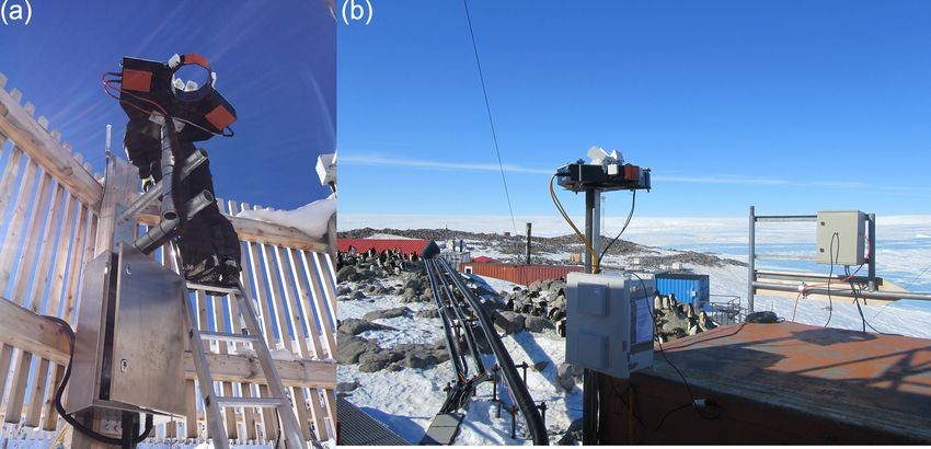
368                                                                          M. Schaer et al.: Blowing snow in MASC images

been shown to be valuable to monitor drifting and blowing          on a manually built validation set. The paper is organized as
snow fluxes (e.g., Bellot et al., 2011). Remote sensing and        follows: Sect. 2 introduces the data sets used to develop the
lidar systems in particular have recently been used to charac-     method and fit the GMM. Section 3 illustrates the different
terize the occurrence and depth of blowing snow layers, ei-        steps to isolate the particles and extract related features for
ther from space (Palm et al., 2011) or near ground level (Gos-     the clustering task. Section 4 explains the selection of the
sart et al., 2017). Suspended ice particles are under the influ-   most relevant features, the fitting of the GMM and the attri-
ence of the gravitational force proportional to the size cubed     bution of a flag for mixed images. The main results are shown
while the drag force is proportional to the area (size squared).   in Sect. 5. At last, limitations and further improvements are
With a greater area-to-mass ratio, smaller particles are thus      discussed in Sect. 6.
more likely to be lifted in the suspension layer. A compari-
son of 10 different studies of measured and simulated particle
size distributions of blowing snow reveals mean diameters at       2     Instrument and data sets
heights above 0.2 m ranging from 50 to 160 µm (Gordon and
                                                                   2.1    The Multi-Angle Snowflake Camera
Taylor, 2009).
   Blowing snow may also contaminate precipitation ob-             The MASC is a ground-based instrument which automat-
servations collected by ground-based sensors, frequently           ically takes high-resolution and stereoscopic photographs
in Antarctica (e.g., Nishimura and Nemoto, 2005; Gossart           of hydrometeors in free fall while measuring their fall ve-
et al., 2017), where winds are strong and frequent, but            locity. Its working mechanism is only summarized here-
also in snowy regions in general (Rasmussen et al., 2012;          after, as more details and explanations can be found in Gar-
Naaim-Bouvet et al., 2014; Scaff et al., 2015). The is-            rett et al. (2012), who provide an extensive description of
sue of snowfall measurement is complex, and the WMO                the instrument. Three high-resolution cameras (2448 pix-
promoted intercomparison projects to evaluate various sen-         els × 2048 pixels), separated by an angle of 36◦ , are attached
sors and define standard setups and protocols over the last        to a ring structure and form altogether the imaging unit (see
two decades, as illustrated in Goodison et al. (1998) and          Fig. 1). The focal point is located inside the ring at about
the recent SPICE project (http://www.wmo.int/pages/prog/           10 cm from each camera (with a focal length of 12.5 mm).
www/IMOP/intercomparisons/SPICE/SPICE.html, last ac-               Particles falling through the ring and detected by the two hor-
cess: 28 January 2020).                                            izontally aligned near-infrared emitter–receiver arrays trig-
   The Multi-Angle Snowflake Camera (MASC) is a ground-            ger the three flashes and the three cameras. The cameras’
based instrument designed to automatically capture high-           apertures and exposure times were adjusted in order to max-
resolution (∼ 33.5 µm) photographs of falling hydrometeors         imize the contrast on hydrometeor photographs while pre-
from three different angles (Garrett et al., 2012). The MASC       venting motion blur effects, leading to a resolution of about
has been used in previous studies to investigate snowflake         33.5 µm and a sampling area of about 8.3 cm2 (see Praz et al.,
properties (Garrett et al., 2015; Grazioli et al., 2017) and to    2017). The maximum frequency of triggering is 3 Hz, which
help interpret weather radar measurements (Kennedy et al.,         is three image triplets per second (see Fig. 6).
2018). Interestingly, blowing snow particles also trigger the         These specifications can be compared to the snow particle
MASC motion detector system (see Sect. 2.1), producing             counter (SPC) which has been used in many studies of blow-
many images in windy environments. In addition to hydrom-          ing snow (e.g., Nishimura and Nemoto, 2005; Gordon and
eteor classification techniques based on MASC images (e.g.,        Taylor, 2009; Kinar and Pomeroy, 2015; Guyomarc’h et al.,
Praz et al., 2017), the ability to discriminate between im-        2019) and can be considered as the reference instrument for
ages composed of blowing snow and precipitation particles          monitoring blowing snow (e.g., Crivelli et al., 2016). The
would therefore be relevant to characterize blowing snow, to       SPC has a control volume of 2 mm × 25 mm × 0.5 mm and
provide reference observations to improve its remote sensing       assigns particles into 32 diameter classes between 50 and
and to obtain more accurate snowfall estimates from ground-        500 µm. It provides information on particle diameter (assum-
based sensors. More generally, detailed information about          ing a spherical shape), particle number and particle mass flux
the type of particles extracted from pictures collected by a       usually at a 1 s resolution (but raw data are measured at up
MASC will enable us to further investigate the complex in-         to 150 kHz, Nishimura et al., 2014). For more information
teractions between wind, snowflakes and snowpack close to          about the SPC, the reader is referred to the articles mentioned
the surface in cold and windy regions.                             above.
   This article presents a new method to automatically de-
termine if an image from the MASC (and potentially other           2.2    Data sets
imaging instruments) is composed of blowing snow particles,
precipitating hydrometeors (snowflakes and ice crystals) or a      The MASC data used to implement and validate the present
mix of both. The classification is accomplished by means of        algorithm were collected during three field campaigns. The
a Gaussian mixture model (GMM) with two components, fit-           first one took place in Davos, Switzerland, from Octo-
ted on a set of representative MASC images and evaluated           ber 2015 to June 2016. The MASC was placed at 2540 m a.s.l

The Cryosphere, 14, 367–384, 2020                                                       www.the-cryosphere.net/14/367/2020/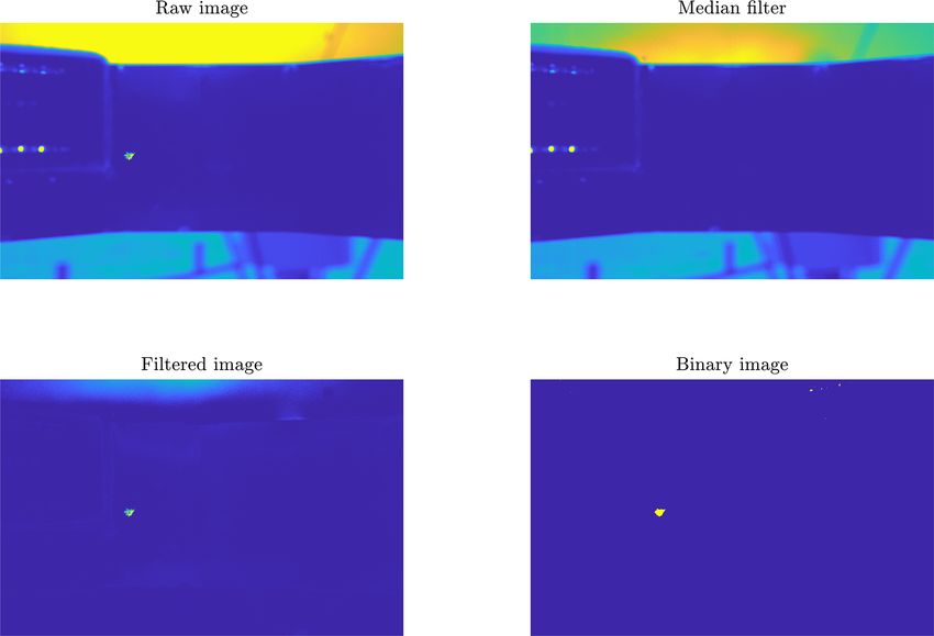
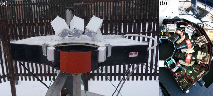
M. Schaer et al.: Blowing snow in MASC images                                                                                          369

Figure 1. (a) Side view of the MASC with the three flash lamps in white on top and the two detectors as white boxes on the side of the metal
ring (in black and red in front). (b) Top view of the inside of the MASC, with the three cameras clearly visible.

in a double-fence intercomparison reference (DFIR; see                  snow events, the number of images captured by the MASC
Fig. 2a), designed to limit the adverse effect of wind on the           was much larger than during precipitation events (more than
measuring instruments in its center (Goodison et al., 1998).            one image per second; see Fig. 6). Potential pure blowing
The MASC was about 3 m above ground. The two other cam-                 snow events were selected when the MASC image frequency
paigns took place at the French Antarctic Dumont d’Urville              and wind speed were higher than their respective median es-
(DDU) station, on the coast of Adélie Land, from Novem-                 timated over the whole campaign (to select relatively high
ber 2015 to February 2015 and from January to July 2017, in             values), and no precipitation was detected during the preced-
the framework of the Antarctic Precipitation, Remote Sens-              ing hour. Only events for which these criteria applied for over
ing from Surface and Space project (http://apres3.osug.fr,              an hour consecutively were kept. To highlight pure precipi-
last access: 28 January 2020) (Grazioli et al., 2017; Genthon           tation, the principle was the same but the criteria were an
et al., 2018). The instrument was deployed on a rooftop at              image frequency and a wind speed lower than the median as
about 3 m above ground (see Fig. 2b). A collocated weather              well as a MRR precipitation rate greater than zero. The MRR
station and a micro rain radar (MRR) were also installed.               has a certain detection limit, so it was noticed that events se-
Nearly 3 million images were collected during these mea-                lected as blowing snow could also occur during undetected
surement campaigns altogether.                                          light precipitation. As a result, images from all events were
   From this large number of data, subsets of pure precip-              rapidly checked visually, and the campaign logbook was con-
itation and pure blowing snow images were manually se-                  sulted to ensure that the selection was consistent and coher-
lected and further analyzed to choose relevant descriptors              ent. In both cases, some events had to be removed because of
and fit a two-component GMM. The task of selecting a suffi-             obvious mixing of blowing snow and hydrometeors.
cient number of representative images for both classes turned              As the MASC was deployed inside a DFIR in Davos, no
out to be more complicated than expected, in particular for             blowing snow events were selected from this campaign. Al-
the Antarctic data set in which mixed images are very fre-              though the DFIR is supposed to shelter the inner instruments
quent. Gossart et al. (2017) used ceilometer data collected at          from wind disturbances, we noticed that many images do not
the Neumayer (coastal) and Princess Elizabeth (inland) sta-             solely contain pure hydrometeors. From a webcam monitor-
tions in East Antarctica to investigate blowing snow, and they          ing the instrumental setup, we noticed that the fresh snow ac-
suggest that more than 90 % of blowing snow occurs dur-                 cumulated on the edges and borders of the wooden structure
ing synoptic events, usually combined with precipitation. For           of the DFIR was frequently blown away towards the sensor.
the sake of generalization, a large number of representative            To enlarge the precipitation subset, events with high snowfall
events were selected across the three campaigns. The goal               rate but not affected by outliers of fresh wind-blown snow
was to cover a wide range of hydrometeors types and a wide              were added. Finally, some sparse images of obvious pure hy-
range of snowfall intensities for the precipitation subset. Sim-        drometeors in the middle of mixed events were also included
ilarly, a wide range of wind speeds and concentrations were             in the training set. In total, each subset contained 4263 im-
considered to build the blowing snow subset. From the cam-              ages and, despite possible remaining (limited) uncertainty in
paigns in Antarctica, pure blowing snow and hydrometeor                 the exact type of images, is assumed to be accurate and re-
events were highlighted by comparing time series of MASC                liable enough to serve as reference for the evaluation of the
image frequency, wind speed and MRR-derived rain rate, as               proposed technique (see Fig. 8 and Sect. 4.2).
illustrated in Fig. 3. It was noticed that during strong blowing

www.the-cryosphere.net/14/367/2020/                                                               The Cryosphere, 14, 367–384, 2020
370                                                                                 M. Schaer et al.: Blowing snow in MASC images

Figure 2. Experimental setup conditions of the MASC in a DFIR near Davos (a) and on top of a container at Dumont d’Urville (b).

Figure 3. Time series and scatter plots of MASC image frequency, wind speed (measured at 10 m) and MRR-derived rain rate for the
Antarctica 2015–2016 campaign. The gray shading indicates days during which time steps have been selected for the training set as blowing
snow (dark gray) or precipitation (light gray). In the bottom scatter plots, the markers figure the selected blowing snow and precipitation time
steps. Points on the x axis in the left scatter plot are potential candidates for pure blowing snow.

3     Image processing                                                    cameras, many MASC pictures contain multiple particles
                                                                          distributed over the entire image, especially when blowing
3.1    Particle detection                                                 snow occurs. In fact, the number of particles appearing on
                                                                          a single image is a key characteristic to distinguish between
The MASC instrument and the collected images are de-                      precipitation and blowing snow. As a result, it was deemed
scribed in Sect. 2.1. Although a single particle activates the

The Cryosphere, 14, 367–384, 2020                                                                 www.the-cryosphere.net/14/367/2020/
M. Schaer et al.: Blowing snow in MASC images 371
Table 1. Campaigns and dates of selected events for the blowing
snow (BS) and precipitation (P) subsets.
Antarctica 2015–2016 Antarctica 2017 Davos 2015–2016
11 Nov BS 8 Feb BS 23 Feb P
22 Nov P 9 Feb BS 25 Feb P
15 Dec P 18 Feb BS 4 Mar P
16 Dec P 19 Feb BS 5 Mar P
30 Dec P 16 Mar P
2 Jan P 25 Mar P
11 Jan P
28 Jan BS
essential to detect all particles in each image rather than the
triggering one only (which is sometimes unidentifiable). A
key challenge of this approach was to get rid of the noisy
background. For this purpose, a median filter was used. The
brightness of the background strongly depends on the lumi-
nosity at the instant of the picture, which varies according to Figure 4. Raw image, median filter, filtered image and final binary
the time of day and can change abruptly in partly cloudy con- image for an example of blowing snow particles. The image size
ditions when the sun suddenly appears from behind a cloud. is 2448 pixels × 2048 pixels, corresponding to 82 mm × 68.6 mm.
As a result, the median filter shows better performance to re- Original MASC images are in gray shades, but the color scheme
move the background when systematically recomputed over used here aims to enhance contrast and details for visual purposes.
a small number of consecutive images. Assuming that snow
particles rarely appear at the exact same position in several
consecutive images, the median filter was chosen to be com-
puted over blocks of five images per camera angle. To en-
sure complete removal of the background when its bright-
ness is greater that the corresponding median, a factor of
1.1 was applied to the filter. Finally, as some limited residual
noise can still remain in the filtered image, a small detection
threshold of 0.02 grayscale intensity was applied to isolate
the snow particles. Masks of the sky and reflecting parts of
the background (i.e., metallic plates) were created for each
camera. The multiplication factor and detection threshold are
increased in the regions delineated by the masks if the normal
filtering leads locally to more pixels detected that one can ex-
pect from real particles. These steps are illustrated in Figs. 4
and 5. Issues in the filtering may occur if consecutive images
are separated by a period of time during which the ambient
luminosity has changed significantly (e.g., before/after the
sunrise or sunset). An example is shown in Fig. B1 in Ap-
pendix B.
3.2 Feature extraction Figure 5. Raw image, median filter, filtered image and final binary
image for an example of a hydrometeor. The color scheme is used
Machine-learning algorithms require a set of variables, com- to enhance details for visual purposes.
monly called features or descriptors, upon which the clas-
sification is performed. Because of the fragmentation of ice
crystals when hitting the snow surface (e.g., Schmidt, 1980; et al., 2014). In this study, various quantitative descriptors
Comola et al., 2017), blowing snow is expected to be charac- were therefore calculated according to four different cate-
terized by much smaller particle size and much higher par- gories: the number of particles and their spread across the
ticle concentration than snowfall (e.g., Budd, 1966; Budd image, the size of the particles, the geometry of the particles,
et al., 1966; Nishimura and Nemoto, 2005; Naaim-Bouvet and the frequency at which the images are taken.
www.the-cryosphere.net/14/367/2020/ The Cryosphere, 14, 367–384, 2020372 M. Schaer et al.: Blowing snow in MASC images
Since it is difficult to exactly guess which descriptors are Table 2. Selected features and corresponding S values.
the most adequate to differentiate between blowing snow
and precipitation images, an extensive collection of fea- Feature name S
tures was extracted from the blowing snow and precipita- Image frequency 4.43
tion subsets and compared. The selection of the most rel- Cumulative distance transform 2.89
evant ones is explained in the next section. As the classi- Maximum diameter quantile 0.7 1.71
fication is performed at the image level, we need features Squared fractal index quantile 0 3.81
at the same level, and the information on the geometry and
size of each detected particle in the considered image must
hence be transformed into a single descriptor for that im- gle particle, even particularly large, will have a high value.
age. Consequently, quantiles ranging from 0 to 1 and mo- This descriptor is more robust to image-processing issues
ments from 1 to 10 were computed out of the distribution than the raw number of particles, as illustrated in Fig. B2
of the considered feature within the image. The image fre- in Appendix B.
quency is a descriptor independent of the content of the Concerning the size distribution of the particles detected in
image and thus from the detection of particles. It is there- an image, the quantile 0.7 of the maximum diameter was se-
fore not affected by potential image-processing issues. As lected (because it has the highest S value among the different
each image comes with its attributed timestamp, the average quantiles tested). The maximum diameter (Dmax ) represents
number of images per minute was calculated with a mov- the longest segment between two edges of a particle (see Praz
ing window. The full list of all computed descriptors is dis- et al., 2017, for more details). A logarithmic transformation
played in Appendix A. The extraction of features was con- of this feature was performed to make the distributions of
ducted with the MATLAB Image Processing Toolbox, in par- the two classes more Gaussian. The minimum (i.e., quantile
ticular the function regionprops (https://ch.mathworks. 0) squared fractal index showed the greatest S value (hence
com/help/images/ref/regionprops.html, last access: 28 Jan- discrimination potential) among the features related to the
uary 2020). particle geometry indices. The fractal index (FRAC) is de-
fined according to the formula proposed by McGarigal and
4 Classification Marks (1995) in the context of landscape-pattern analysis. It
was also more recently used to quantify stand structural com-
4.1 Feature selection and transformation plexity from terrestrial laser scans of forests (Ehbrecht et al.,
2017).
Selecting a relevant set of features and avoiding redundancy Due to its different nature, the image frequency descrip-
is essential for accurate classification, regardless of the clas- tor was selected by default, but it is worth noting that it
sification algorithm. For each of the four categories of de- has the highest S value (Eq. 1) among all descriptors (Ta-
scriptors previously mentioned, the most relevant one (ac- ble 2). The marginal distributions of the selected descriptors
cording to the criterion explained below) was kept. The de- for the training set are shown in Fig. 6 to provide an idea
scriptor maximizing the interclusters-over-intraclusters dis- of their respective magnitude and variability, as well as to
tance described in Eq. (1) was selected. This quantity repre- illustrate their discrimination potential. As noted above, the
sents the distance between the mean of the blowing snow and image frequency is the most informative descriptor to distin-
precipitation distributions (µBS and µP respectively), nor- guish blowing snow and precipitation.
malized by the sum of their respective standard deviations In summary, four descriptor categories (related to parti-
(σBS and σP respectively). cle size, particle geometry and particle distribution within
the image, and image frequency) have been defined to dis-
|µBS − µP | tinguish images collected during blowing snow or snowfall,
S= 1
. (1)
2 (σBS + σP ) based on the expected differences in particle size and con-
centration between the two. A number of descriptors were
For the features describing the number of detected par- estimated from each image by computing various quantiles
ticles and their spread across the image, the cumula- and moments of the distributions of geometric properties of
tive distance transform was kept. It represents the sum the particles in the considered image. One descriptor from
over each entry of the distance transform matrix (https:// each of the four categories defined above (listed in Table 2)
ch.mathworks.com/help/images/ref/bwdist.html, last access: was then selected to be further used for classification as the
28 January 2020) of the binary image. The distance trans- one maximizing the interclusters-over-intraclusters distance
form matrix has the same dimensions as the binary image and defined in Eq. (1).
computes, for each pixel, the Euclidean distance to the near-
est 1 element (i.e., the nearest particle). As a result, an image
with many particles well distributed over its entire surface
will have a low cumulative distance transform, while a sin-
The Cryosphere, 14, 367–384, 2020 www.the-cryosphere.net/14/367/2020/M. Schaer et al.: Blowing snow in MASC images 373
Figure 6. Histograms of selected descriptors for the training blowing snow and precipitation subsets.
4.2 Model fitting provide posterior probabilities on the cluster assignments and
thus allow for soft clustering (i.e., probabilistic assignment).
The choice for the binary classification task was made on In the context of the present study, this is absolutely rele-
a Gaussian mixture model, an unsupervised learning tech- vant as there exists a whole continuum of in-between cases
nique that fits a mixture of multivariate Gaussian distribu- of mixed images. It should be noted that the descriptors were
tions to the data (see Murphy, 2012; McLachlan and Basford, selected using a reference set (see previous section), but the
1988; Moerland, 2000, for more details). The mathematical clustering conducted by means of the GMM is itself unsu-
description of a multivariate normal distribution is provided pervised.
in Eq. (2). A two-component GMM with unshared full covari-
ance matrices was thus fitted to the four-dimensional
1
N (x|µ, 6) = (x = {f1 , f2 , f3 , f4 }, where fi represents the four features
(2π )D/2 |6|1/2 listed in Table 2) data composed of the blowing snow and
1 precipitation subsets. The MATLAB Statistics and Machine
exp{− (x − µ)T 6 −1 (x − µ)}, (2)
2 Learning Toolbox was used for this purpose, and the model
parameters were estimated by maximum likelihood via
where x is a Gaussian multivariate random variable of di-
the expectation–maximization (EM) algorithm (https://ch.
mension D, µ its mean and 6 its covariance matrix, with T
mathworks.com/help/stats/gaussian-mixture-models-2.html,
the transpose operator.
last access: 28 January 2020). The features were stan-
The choice of an unsupervised approach is based on sev-
dardized before fitting the model. The mixing weights
eral reasons. First, unsupervised methods do not depend upon
(or component proportions) were artificially set to 0.5 by
labels. Hence, it is not required to ensure correct labeling of
randomly removing 80 data points from the training set and
each image in the training set. As mentioned earlier, many
fitting again the GMM to have perfectly balanced classes.
images are composed of a mix of blowing snow and precip-
This step is essential as the model will then be used to
itation, and it is thus difficult to guarantee the objectivity of
classify new images (possibly from other campaigns). There
all given labels. Second, a clear separation observed between
are no reasons to give more weight to one component, as the
the two subsets would be statistically highly significant as
relative proportion of blowing snow and precipitation images
no prior information is provided to the learning algorithm
strongly depends on the campaign location. The posterior
about the classes. Third, for low-dimension problems, unsu-
probabilities are computed using the Bayes rule (Murphy,
pervised methods are sometimes less prone to overfitting and
have a better potential for generalization. A main advantage
of the GMM compared to other unsupervised methods is to
www.the-cryosphere.net/14/367/2020/ The Cryosphere, 14, 367–384, 2020374 M. Schaer et al.: Blowing snow in MASC images
2012): is used indicates a data set large enough for a reliable fitting
of the GMM, without overfitting.
P (x i |zi = k, θ )P (zi = k|θ )
P (zi = k|x i , θ ) = , (3)
P (x i |θ ) 4.3 Flag for mixed images
where zi is a discrete latent variable taking the values As mentioned earlier, an asset of using a GMM model is
1, . . ., K and labeling the K Gaussian components. P (zi = the posterior probabilistic information that could help esti-
k|x i , θ ) is the posterior probability that point i belongs to mate the degree of mixing of an image. Data points located
cluster k (also known as the “responsibility” of cluster k for close to the decision boundary in the multidimensional space
point i). P (x i |zi = k, θ ) corresponds to the density of com- are likely to be composed of a mix of blowing snow parti-
ponent k at point i (i.e., N (x i |µk , 6 k )), and P (zi = k|θ ) cles and hydrometeors. However, distributions of posterior
represents the mixing weight (also denoted πk ). Note that probabilities computed over thousands of new images from
the πk ’s are positive and sum to 1. θ refers to the fitted entire campaigns appeared to be stretched out on both ends
parameters of the mixture model {µ1 , . . ., µk , 6 1 , . . ., 6 K , of the domain (i.e., close to 0 or 1), and not many images
π1 , . . ., πK }. P (x i |θ ) is the marginal probability at point i, were present in between. This is probably due to the nature
which is simply the weighted sum of all component densi- of the descriptors and the resulting shapes and relative po-
ties: sitions of the Gaussian distributions. In order to investigate
K
X this issue, an additional set of images corresponding to mixed
P (x i |θ ) = πk N (x i |µk , 6 k ). (4) cases was built: it exhibited clear differences in the posterior
k=1 probabilities with the pure blowing snow and pure precipita-
As the concern of this study is on two components only, tion subsets. This differentiation was however around 10−6
a more compact notation will be used for the rest of the ar- (or 1 − 10−6 ), which is not so informative as such. Conse-
ticle. The latent variable z will be replaced by kP and kBS quently, it was decided to define a new index similar to the
to refer to the precipitation and blowing snow clusters, re- posterior probability of belonging to the blowing snow com-
spectively. The term θ , which denotes the model parame- ponent but more evenly distributed across the range ]0, 1[.
ters, will be left implicit. Assuming we are at first interested The new index uses the negative logarithm of the posterior
in performing some hard clustering (i.e., single label to a probabilities multiplied by the marginal probability. Taking
given image), an image will be classified as blowing snow if the log of Eq. (3) for kBS , we have (the same applies for kP )
P (kBS |x i ) > P (kP |x i ). That is to say, if the posterior proba-
− log[P (kBS |x i )P (x i )] = − log[P (x i |kBS )P (kBS )]. (5)
bility of belonging to the blowing snow cluster is greater than
0.5, an image will be classified as such (because the posterior Noting that the term P (x i |kBS ) on the right-hand side is
probabilities sum to 1). The model performance was assessed N (x i |µBS , 6 BS ), one can substitute Eq. (2) into the above
by simply labeling the data points according to its initial sub- expression, which yields
set. An overall accuracy of 99.4 % and a Cohen kappa score
of 98.8 % were achieved. The Cohen kappa statistic adjusts − log[P (kBS |x i )] − log[P (x i )] =
the accuracy by accounting for correct predictions occurring 1 1
by chance (Byrt et al., 1993). These high values indicate a (x i − µBS )T 6 −1
BS (x i − µBS ) + log(|6 BS |)
2 2
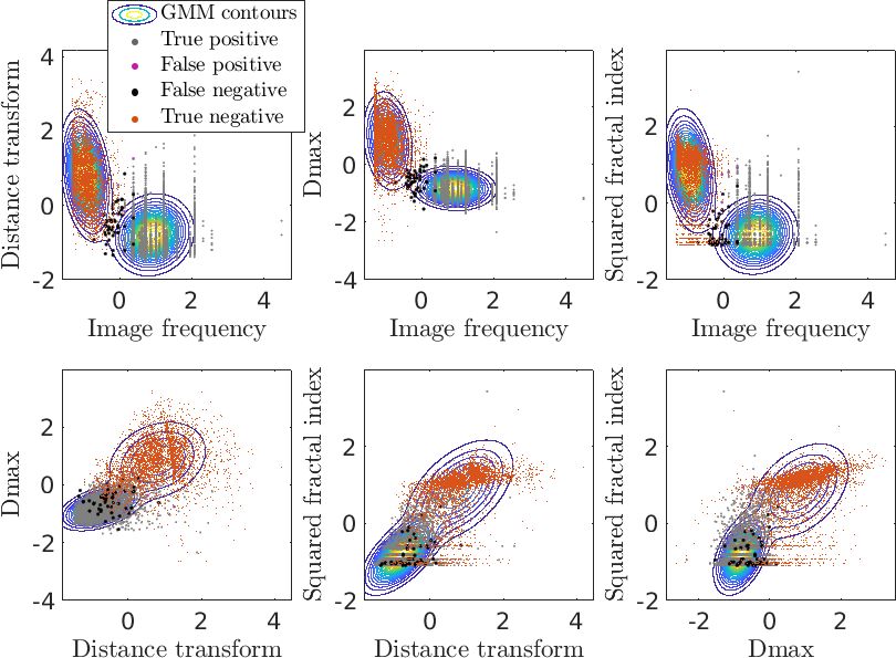
very good performance of the fitted GMM. Figure 7 presents D
the fitted Gaussian components as well as the reference val- + log(2π ) − log(P (kBS )). (6)
2
ues (not used in the fitting) for each of the six possible pairs
of the four descriptors. It clearly illustrates the performance The quadratic term on the right-hand side is the Maha-
of the fitted GMM and the discriminative power of the de- lanobis distance, which is a distance that uses a 6 −1 norm.
scriptor related to image frequency. Hence, it represents the distance between point x i and the
To investigate the stability of the Gaussian components, center of the distribution, corrected for correlations and un-
the precipitation and blowing snow subsets were both ran- equal variances in the feature space (De Maesschalck et al.,
domly permuted and divided into 10 equal parts. Ten new 2000). The second term is related to the determinant of the
training sets of a balanced amount of each subset were cre- covariance matrix and equals −3.94 for the blowing snow
ated, and a new GMM was fitted. Figure 8 shows on the component and −2.59 for the precipitation one. The two last
top line the boxplots of the Gaussian component parame- terms are constant and sum to 4.37 (the component propor-
ters µd and σ d (i.e., diagonal entries of 6) for each of the tions were set to 0.5 and D = 4). The right side of Eq. (6)
four dimensions. The boxplots show a limited variability for is also known as the quadratic discriminant function (QDF,
each feature (below 10 %), indicating a reasonable stability Kimura et al., 1987), commonly noted gk (x i ). The minus in
of the fitted parameters. In addition, the bottom line of Fig. 8 front of the logarithm on the left side of Eq. (6) is used to
presents the learning curves, and their fast convergence to the return positive values and facilitate subsequent graphical in-
same horizontal line when more than 30 % of the training set terpretations. Note that the constant term D2 log(2π ) is often
The Cryosphere, 14, 367–384, 2020 www.the-cryosphere.net/14/367/2020/M. Schaer et al.: Blowing snow in MASC images 375
Figure 7. GMM contours and data points projected on the 2-D planes. The colors correspond to the four entries of the confusion matrix. The
predictions result from the clustering and the ground truth is the given labels.
removed, but in this case it ensures that gk (x) is positive, (increasing it) or less (decreasing it) strict on the classifica-
even for a Mahalanobis distance of zero. Figure 9 displays tion as pure blowing snow or pure precipitation, depending
a scatter plot of the quadratic discriminant values of both on the intended application.
components for the whole training set. The proposed index To ease reading and interpretation, a mixing index λm is
is defined as the angle of the vector representing a data point introduced by linearly rescaling between 0 and 1 the ψ index
on the scatter plot, normalized by π2 . It is thus computed as of the images flagged as mixed (i.e., λm is not defined for
follows: pure precipitation or pure blowing snow images):
2 − log[P (kP |x i )P (x i )] λm = 0.5
0.5−ψP0.9 (ψ − ψP0.9 ) if ψ ∈ (ψP0.9 , 0.5),
ψ = arctan . (7) 0.5 (8)
π − log[P (kBS |x i )P (x i )] = 0.5−ψBS0.1 ((1 − ψBS0.1 ) − ψ) if ψ ∈ [0.5, ψBS0.1 ).
This normalized angle is bounded in ]0, 1[, with values The mixing index also respects the hard clustering assign-
close to 1 (respectively 0) indicating a strong membership ment boundary at 0.5: λm > 0.5 indicates that the image con-
of the considered image (and not the respective proportions tains a mix of blowing snow and precipitation particles, but
within this image) to the blowing snow (respectively precip- it is closer overall to blowing snow and vice versa. Images
itation) clusters. It is closely related to the asymmetry of the with a normalized angle outside the two mixed thresholds
Mahalanobis distances between a point x i and the centers have an undefined (NaN) index of mixing and are considered
of the two Gaussian distributions but corrected by the term as pure blowing snow particles or pure hydrometeors. Results
1
2 log(|6|), which is different for the two components. The are provided treating all images independently, but the ψ in-
advantage of using the index in this form, rather than deriving dex can also be averaged among the three camera angles to
it from the Mahalanobis distances alone, is to respect the de- provide a unique value per image identifier as well. The me-
cision boundary given by the maximum a posteriori (MAP) dian of the range (max – min) covered by the ψ values from
rule. This means a posterior probability of 0.5 yields a ψ in- the three individual views is about 0.08 in Davos and 0.05
dex of 0.5. Finally, quantiles 0.9 (ψP0.9 ) and 0.1 (ψBS0.1 ) of at Dumont d’Urville, indicating a limited variability between
the ψ index distributions of the points classified as precipi- the three views.
tation and blowing snow, respectively, are retained as thresh- In summary, the classification as a mixed case is based on
olds to flag potential mixed images. The idea is to allow, for the angle characterizing the considered MASC image in the
both classes, 10 % of the training set images to be flagged as 2-D space formed by the axis related to pure blowing snow
mixed. This value is qualitatively supported by the distribu- on the one hand and the one related to pure precipitation on
tion shown in Fig. 9. It can be changed by the user to be more the other hand. A mixing index λm is finally computed by lin-
www.the-cryosphere.net/14/367/2020/ The Cryosphere, 14, 367–384, 2020376 M. Schaer et al.: Blowing snow in MASC images
Figure 8. (a, b) Stability of the parameters µ and σ (diagonal entries of 6) for the two Gaussian components. The boxplots show the
distributions of these parameters for each dimension, after fitting the GMM on a 10-fold random split of the training set. The feature number
follows the order given in Table 2. (c) Learning curves for the fitted GMM, showing the evolution of the train and Cohen’s kappa test as
a function of the proportion of the training samples used. The shaded areas correspond to the 25–75th percentile range computed over 40
iterations of 70 %–30 % random train-test splitting, and the bold lines are the medians.
early rescaling the normalized angle over the range of values Table 3. Percentages of MASC images per category.
corresponding to mixed cases.
Class Antarctica Davos
(Jan–Jul 2017) (Dec 2015–Mar 2016)
5 Results Pure blowing snow 36.5 % 0.6 %
Pure precipitation 7.2 % 39.2 %
The method presented (and fitted) in the previous sec- Mixed blowing snow 39.1 % 20.9 %
tions is now applied to the entire Antarctica 2017 cam- Mixed precipitation 17.2 % 39.3 %
paign (January–July 2017) and to the entire Davos cam-
paign (December 2015–March 2016). About 2 × 10⁶ images
for Antarctica and 8.5 × 10⁵ for Davos were classified. Ta-
ble 3 summarized the outcome in terms of respective pro- there are much more points around the one–one line (Fig. 9a)
portions of pure blowing snow, pure precipitation, mixed and a small mode around 0.5 (Fig. 9b) for the entire cam-
blowing snow, and mixed precipitation for the Antarctic and paign than for the training set (built with much fewer mixed
Alpine data sets. As expected, the occurrence of blowing cases). It is also clear from Fig. 10b that blowing snow and
snow (pure + mixed) is much more frequent at Dumont mixed blowing snow are more frequent than precipitation and
d’Urville (75.6 %) than at Davos (21.5 %, out of which only mixed precipitation.
0.6 % if of pure blowing snow). Figure 11 is similar to Fig. 10 but for the entire Davos
Figure 10a shows the distribution of the collected MASC data set. In comparison with Fig. 10, the occurrence of pre-
images in the space formed by the two quadratic discriminant cipitation is much larger (and blowing snow much smaller),
(one for blowing snow, one for precipitation), and Fig. 10b which is to be expected given the difference in geographic
shows the distribution of the normalized angle for the entire context (Alps vs. Antarctica) and experimental setup (wind-
Antarctica 2017 campaign. A clear difference with Fig. 9 is protected vs. no wind shield). It should be noted that mixed
the large proportion of values corresponding to mixed cases: cases are relatively frequent and that blowing snow still hap-
The Cryosphere, 14, 367–384, 2020 www.the-cryosphere.net/14/367/2020/M. Schaer et al.: Blowing snow in MASC images 377 Figure 9. (a) Scatter plot of the quadratic discriminant values of both components for the training set. (b) Probability density func- Figure 10. (a) Scatter plot of the quadratic discriminant values of tions (PDF) of the normalized angle for the precipitation and blow- both components for the entire Antarctica 2017 campaign. (b) Dis- ing snow subsets and thresholds to identify mixed images. tribution of the normalized angle and corresponding classification. pens in Davos although the MASC was located in a wind a temporal resolution high enough to capture the dynamics shielding fence. of the event is an interesting feature for regions where both Beyond global statistics on various data sets as presented are frequently associated. above, the proposed approach can also be used to investigate Considering the full Antarctic and Alpine data sets, it is the type of images at high temporal resolutions. Figure 12 interesting to analyze the potential differences in their char- shows an example of the output of the algorithm and corre- acteristics. Figure 14 presents the distributions of the four sponding images for a few time steps during a mixed event. descriptors as in Fig. 6 but estimated from the entire data It illustrates the capability of the proposed approach to dis- sets and not only the training sets (for images classified as tinguish blowing snow, precipitation and mixture in individ- pure blowing snow or pure precipitation). It can be seen that ual MASC images separated by a few seconds (and hence while the differences are limited for precipitation (slightly the contribution of the features other than image frequency). more frequent and larger in Davos than in Dumont d’Urville), Over a longer time period, Fig. 13 displays the evolution of they are significant for blowing snow: the blowing snow par- the normalized angle for a mixed event during the Antarc- ticles appear less fragmented (larger size and fractal index), tica 2017 campaign. From roughly 09:00 to 12:00, the types less scattered within the images (larger distance transform) precipitation and mixed are dominant, while between 12:00 and with lower image frequencies in Davos. It should be re- and 14:00 the three types (precipitation, mixed and blow- called that the MASC was located in a wind-protecting fence ing snow) occur simultaneously. This is to be expected at in Davos, so first the occurrence of blowing snow is much DDU where katabatic winds blow very frequently, even dur- smaller (0.6 vs. 36.5 %), and second it is likely related to ing precipitation (e.g., Vignon et al., 2019). From 14:00 to fresh snow blown away from the top of the nearby fence. 22:00, blowing snow becomes dominant (because of stronger The MASC resolution (33.5 µm) and thresholding (mini- winds). After 22:00, mixed cases dominate and some images mum 3 pixels in area) during image processing lead to an corresponding to precipitation are detected towards the end image resolution not high enough to capture in full detail the of the event. The possibility of identifying MASC images geometry of blowing snow particles. It is nevertheless inter- corresponding to precipitation, blowing snow or a mixture at esting to plot the distribution of the measured sizes (asso- www.the-cryosphere.net/14/367/2020/ The Cryosphere, 14, 367–384, 2020
378                                                                          M. Schaer et al.: Blowing snow in MASC images

                                                                    Figure 12. Consecutive MASC images from Davos and their re-
                                                                    spective classification label, normalized angle and mixing index.
                                                                    Label 1 is for blowing snow. A NaN mixing index means pure hy-
                                                                    drometeor (or pure blowing snow). A mixing index close to 1 (top-
                                                                    left image) means that it is near pure blowing snow, while a value
Figure 11. Same as Fig. 10 for the entire Davos campaign.           close to 0 (bottom-right image) indicates proximity to pure precipi-
                                                                    tation.

ciated with the MASC sampling area) for blowing snow and
precipitation cases and compare it to existing values in the lit-
erature. Figure 15 displays the distributions of the measured
size (quantified here as Dmax ) for blowing snow and precip-
itation in Antarctica, as well as precipitation in the Swiss
Alps. To help visualize the sometimes overlapping empirical
distributions, the fitted gamma distributions are also plotted.
The units are given in millimeters, with the approximation
that 1 pixel is ∼ 33.5 µm.
   As expected, the size distribution of blowing snow corre-
sponds to smaller sizes than precipitation: the mode is around
0.2 mm for blowing snow and 0.3 to 0.4 mm for precipitation.
More importantly, the right tail of the distribution is much        Figure 13. Time series of classified MASC images and correspond-
larger for precipitation than for blowing snow. It should also      ing ψ values (averaged over the three views) for a mixed event dur-
be noted that the size is slightly larger in the Alpine data set    ing the Antarctica 2017 campaign.
(as illustrated by the slightly larger mode of the fitted gamma
distributions).
   Nishimura and Nemoto (2005) provide size distributions           ing blowing snow, some may be out of focus and artificially
of blowing snow and precipitation measured in Antarctica at         appear larger than they are. So we expect the blowing snow
Mizuho station using a SPC. The bimodality obtained when            features extracted from MASC data to be biased towards
combining blowing snow and precipitation data in Fig. 15 is         larger particles. It should also be noted that the sampling ar-
in general agreement with the mixed case in their Fig. 10.          eas of the two instruments are different (see Sect. 2.1), and
However, the mode for blowing snow appears at a lower size          this could partly explain the differences in the obtained dis-
(below 50 µm in their Fig. 7 at a height of 3.1 m). As men-         tributions.
tioned before, this discrepancy is likely due to the limited ef-       Overall, it appears that the MASC images, processed as
fective resolution in MASC images after processing. In addi-        explained in Praz et al. (2017), are not adapted to a detailed
tion, as there are usually many particles in a single image dur-    study of the geometry of blowing snow particles but are still

The Cryosphere, 14, 367–384, 2020                                                          www.the-cryosphere.net/14/367/2020/
M. Schaer et al.: Blowing snow in MASC images 379
Figure 14. Histograms of selected descriptors for the training blowing snow and precipitation images from the entire Dumont d’Urville and
Davos data sets.
6 Conclusions
A novel method to automatically detect images from the
MASC instrument corresponding to blowing snow is intro-
duced. To classify the images, the method computes four
selected descriptors via image processing. The descriptors
were selected to be relevant for discriminating between blow-
ing snow particles and hydrometeors as well as to be robust
to image-processing artifacts. The classification is achieved
by a two-component Gaussian mixture model fitted on a
subset of 8450 representative images from field campaigns
in Antarctica and Davos, Switzerland. The fitted GMM is
shown to reliably distinguish images corresponding to pure
blowing snow and pure precipitation cases. The GMM pos-
terior probabilities are also mapped into a new index that al-
lows a better identification of mixed images, and a flag sig-
Figure 15. Histograms and fitted gamma distributions of Dmax
nals whether an image is classified as pure hydrometeor, pure
for images classified as pure blowing snow and pure hydrometeors blowing snow or mixed. For mixed images, an index between
from Antarctica and pure precipitation from the Alps. 0 and 1 is proposed to indicate if the image is closer to blow-
ing snow or precipitation. Its evaluation remains qualitative
as there are no quantitative observations that can be used as
relevant to distinguish blowing snow and precipitation, to reference for mixed cases. The outputs are provided for each
characterize mixtures of both and to analyze the dynamics image independently or for each triplet of images (i.e., infor-
of blowing snow at high temporal resolutions. mation combined over the three cameras of the MASC).
Results from a measurement campaign conducted at the
Dumont d’Urville station on the coast of East Antarctica
from January to July 2017 suggest that about 75 % of the im-
ages are affected by blowing snow and that about 36 % may
be composed of blowing snow particles only (Table 3). The
www.the-cryosphere.net/14/367/2020/ The Cryosphere, 14, 367–384, 2020380 M. Schaer et al.: Blowing snow in MASC images results also suggest that about 56 % of the images could be The main limitations of the present method are the as- made of a mix of blowing snow and precipitation particles, sumption of normally distributed features through the use of which support findings that in Antarctica blowing snow is the GMM, the too-coarse resolution of the MASC to prop- frequently combined with precipitation (e.g., Gossart et al., erly capture the small end of the distribution of blowing snow 2017). Moreover, time series of the classified images high- particle size and the dependency of the method on the defined light that blowing snow strongly relies upon fresh snow avail- training set. The latter illustrates the problem of generaliza- ability and often starts shortly after the beginning of precip- tion. Some extremely high intensity snowfall events, higher itation (Fig. 13), which is also consistent with conclusions than the ones observed during the Davos and Antarctica cam- from Gossart et al. (2017). Results from images taken inside paigns, could be erroneously classified as blowing snow with a double-fence intercomparison reference in Davos at 2540 m the current model due to the nature of the descriptors. In a.s.l between December 2015 and March 2016 indicate that, this case, higher-intensity pure snowfall events should be in- despite the sheltering structure, about 60 % of the images cluded in the training set. Another example is the size of the could be affected to some extent by blowing snow particles blowing snow particles. During the campaigns in Antarctica, from adjacent fence ledges. In terms of the percentage of im- the MASC was set up on a rooftop at 3 m a.g.l. Several stud- ages, these numbers tend to be quite large, as the image fre- ies have demonstrated that the size of blowing snow particles quency is usually much higher when strong blowing snow tends to decrease with height (Nishimura and Nemoto, 2005; occurs, but the occurrence is more balanced in terms of time. Nishimura et al., 2014). Consequently, blowing snow parti- As the method was developed and tested on fundamen- cles on images from a MASC that would have been set up tally different campaigns, it may have a general applicability at much higher or lower heights may have a bias relative to to any other MASC images. However, it should be noted that the fitted Gaussian distribution of the blowing snow cluster some descriptors depend on the particular settings (e.g., im- for Dmax . It is thus recommended to follow the procedure de- age size and pixel resolution) used during the aforementioned scribed in this article and fit a new model, if the one provided campaigns, and a new GMM should be fitted if different set- does not perform well in other contexts. tings apply. Further work should be conducted to evaluate if the method can give satisfactory results on images that do not include a timestamp, as the image frequency descriptor could not be utilized. In this case, it could be replaced by one or a couple of other descriptors listed in Table A1 of Ap- pendix A to strengthen the model. The method could also be adjusted to train a model with a supervised learning algo- rithm that provides posterior probabilities such as Bayesian classifiers or logistic regression. However, this would imply some effort to increase the training set. An intercomparison between different machine-learning algorithms and the cre- ation of different validation sets could help gain confidence in the results. The Cryosphere, 14, 367–384, 2020 www.the-cryosphere.net/14/367/2020/
M. Schaer et al.: Blowing snow in MASC images                                                                                             381

Appendix A: Feature extraction

Table A1. Full list of all computed descriptors. Descriptors related to each particle are transformed into a single descriptor for the image
(right column). Selected ones are shown with an asterisk.

    Image frequency∗                                                                                         –
    Number of particles detected in the image                                                                –
    Distance to connect all particles                                                                        –
    Number of particles smaller than a given threshold                                                       –
    Ratio of the area represented by all particles to the area of the smallest polygon encircling them       –
    Cumulative distance transform∗                                                                           –
    Maximum diameter∗                                                                                        quantiles 0–1, moments 1–5
    Particle area                                                                                            quantiles 0–1, moments 1–5
    Particle convex area                                                                                     quantiles 0–1, moments 1–5
    Particle perimeter                                                                                       quantiles 0–1, moments 1–5
    Fractal index (FRAC), fractal index squared∗                                                             quantiles 0–1, moments 1–5
    Gravelius compactness coefficient (ratio of the perimeter to the one of a circle with equivalent area)   quantiles 0–1, moments 1–5

www.the-cryosphere.net/14/367/2020/                                                                 The Cryosphere, 14, 367–384, 2020
382 M. Schaer et al.: Blowing snow in MASC images Appendix B: Image-processing issues The median filter may not perform satisfactorily, for instance when the background luminosity is changing rapidly (see Fig. B1). Similarly, large precipitation particles may split or appear as such in the MASC images (see Fig. B2), leading to poten- tial biases in the number of detected particles. Figure B1. Raw image, median filter, filtered image and final binary image for an example where the median filter does not perform well due to changes in sky luminosity. Some artifacts appear on the top right of the binary image Figure B2. A precipitation particle split into fragments that could be confused with blowing snow particles. The cumulative distance trans- form descriptor is much less affected by such image-processing issues than the number of particles. The Cryosphere, 14, 367–384, 2020 www.the-cryosphere.net/14/367/2020/
M. Schaer et al.: Blowing snow in MASC images                                                                                                 383

Code and data availability. The MASC images and the MATLAB                Crivelli, P., Paterna, E., Horender, S., and Lehning, M.: Quantify-
codes used in the present work are available upon request to the            ing particle numbers and mass flux in drifting snow, Bound.-Lay.
authors.                                                                    Meterol., 161, 519–542, 2016.
                                                                          Das, I., Bell, R. E., Scambos, T. A., Wolovick, M., Creyts, T. T.,
                                                                            Studinger, M., Frearson, N., Nicolas, J. P., Lenaerts, J. T. M., and
Author contributions. MS, CP and AB designed the study; MS per-             van den Broeke, M. R.: Influence of persistent wind scour on the
formed the computation; and all authors contributed to the writing          surface mass balance of Antarctica, Nat. Geosci., 6, 367–371,
of the paper.                                                               https://doi.org/10.1038/NGEO1766, 2013.
                                                                          De Maesschalck, R., Jouan-Rimbaud, D., and Massart, D. L.: The
                                                                            Mahalanobis distance, Chemometr. Intell. Lab., 50, 1–18, 2000.
Competing interests. The authors declare that they have no conflict       Déry, S. J. and Yau, M.: Large-scale mass balance effects of blow-
of interest.                                                                ing snow and surface sublimation, J. Geophys. Res., 107, 4679,
                                                                            https://doi.org/10.1029/2001JD001251, 2002.
                                                                          Ehbrecht, M., Schall, P., Ammer, C., and Seidel, D.: Quantifying
                                                                            stand structural complexity and its relationship with forest man-
Acknowledgements. The authors are thankful to Yves-Alain Roulet
                                                                            agement, tree species diversity and microclimate, Agr. Forest
and Jacques Grandjean from MeteoSwiss, as well as to Claudio
                                                                            Meteorol., 242, 1–9, 2017.
Dùran from IGE Grenoble and to the technical staff from IPEV at
                                                                          Gallée, H., Guyomarc’h, G., and Brun, E.: Impact of snow drift on
the Dumont d’Urville station, for their help in collecting the set of
                                                                            the Antarctic ice sheet surface mass balance: possible sensitiv-
MASC images used in this study, in the framework of the APRES3
                                                                            ity to snow-surface properties, Bound.-Lay. Meterol., 99, 1–19,
project. Christophe Praz was supported by the Swiss National Sci-
                                                                            2001.
ence Foundation (grant 200020_175700).
                                                                          Garrett, T. J., Fallgatter, C., Shkurko, K., and Howlett, D.: Fall
                                                                            speed measurement and high-resolution multi-angle photogra-
                                                                            phy of hydrometeors in free fall, Atmos. Meas. Tech., 5, 2625–
Financial support. This research has been supported by the Swiss            2633, https://doi.org/10.5194/amt-5-2625-2012, 2012.
National Science Foundation (grant no. 200020_175700).                    Garrett, T. J., Yuter, S. E., Fallgatter, C., Shkurko, K., Rhodes, S. R.,
                                                                            and Endries, J. L.: Orientations and aspect ratios of falling snow,
                                                                            Geophys. Res. Lett., 42, 4617–4622, 2015.
Review statement. This paper was edited by Marie Dumont and re-           Genthon, C., Berne, A., Grazioli, J., Durán Alarcón, C.,
viewed by Nikolas Aksamit and two anonymous referees.                       Praz, C., and Boudevillain, B.: Precipitation at Dumont
                                                                            d’Urville, Adélie Land, East Antarctica: the APRES3 field
                                                                            campaigns dataset, Earth Syst. Sci. Data, 10, 1605–1612,
                                                                            https://doi.org/10.5194/essd-10-1605-2018, 2018.
References                                                                Goodison, B. E., Louie, P. Y., and Yang, D.: WMO solid precipita-
                                                                            tion measurement intercomparison, World Meteorological Orga-
Bellot, H., Trouvilliez, A., Naaim-Bouvet, F., Genthon, C., and Gal-        nization Geneva, Switzerland, 1998.
  lée, H.: Present weather-sensor tests for measuring drifting snow,      Gordon, M. and Taylor, P. A.: Measurements of blowing snow, Part
  Ann. Glaciol., 52, 176–184, 2011.                                         I: Particle shape, size distribution, velocity, and number flux at
Bintanja, R.: Snowdrift sublimation in a katabatic wind                     Churchill, Manitoba, Canada, Cold Reg. Sci. Technol., 55, 63–
  region of the Antarctic ice sheet, J. Appl. Mete-                         74, 2009.
  orol.,      40,      1952–1966,        https://doi.org/10.1175/1520-    Gossart, A., Souverijns, N., Gorodetskaya, I. V., Lhermitte, S.,
  0450(2001)0402.0.CO;2, 2001.                                 Lenaerts, J. T. M., Schween, J. H., Mangold, A., Laffineur,
Box, J. E., Bromwich, D. H., Veenhuis, B. A., Bai, L.-S., Stroeve,          Q., and van Lipzig, N. P. M.: Blowing snow detection from
  J. C., Rogers, J. C., Steffen, K., Haran, T., and Wang, S.-H.:            ground-based ceilometers: application to East Antarctica, The
  Greenland ice sheet surface mass balance variability (1988–               Cryosphere, 11, 2755–2772, https://doi.org/10.5194/tc-11-2755-
  2004) from calibrated polar MM5 output, J. Climate, 19, 2783–             2017, 2017.
  2800, 2006.                                                             Grazioli, J., Genthon, C., Boudevillain, B., Duran-Alarcon, C., Del
Budd, W., Dingle, W., and Radok, U.: The Byrd snow drift project:           Guasta, M., Madeleine, J.-B., and Berne, A.: Measurements of
  outline and basic results, in: Studies in Antarctic Meteorology,          precipitation in Dumont d’Urville, Adélie Land, East Antarctica,
  edited by: Rubin, M. J., vol. 9 of Antarctic Research Series,             The Cryosphere, 11, 1797–1811, https://doi.org/10.5194/tc-11-
  American Geophysical Union, 71–134, 1966.                                 1797-2017, 2017.
Budd, W. F.: The drifting of non-uniform snow particles, in: Stud-        Guyomarc’h, G., Bellot, H., Vionnet, V., Naaim-Bouvet, F., Déliot,
  ies in Antarctic Meteorology, edited by: Rubin, M. J., vol. 9 of          Y., Fontaine, F., Puglièse, P., Nishimura, K., Durand, Y., and
  Antarctic Research Series, American Geophysical Union, 59–70,             Naaim, M.: A meteorological and blowing snow data set
  1966.                                                                     (2000–2016) from a high-elevation alpine site (Col du Lac
Byrt, T., Bishop, J., and Carlin, J. B.: Bias, prevalence and kappa, J.     Blanc, France, 2720 m a.s.l.), Earth Syst. Sci. Data, 11, 57–69,
  Clin. Epidemiol., 46, 423–429, 1993.                                      https://doi.org/10.5194/essd-11-57-2019, 2019.
Comola, F., Kok, J. F., Gaume, J., Paterna, E., and Lehning,
  M.: Fragmentation of wind-blown snow crystals, Geophys. Res.
  Lett., 44, 4195–4203, 2017.

www.the-cryosphere.net/14/367/2020/                                                                   The Cryosphere, 14, 367–384, 2020
You can also read