Imaging with CASA Philippe Salomé LERMA, Observatoire de Paris - Credits: (Jérôme Pety, Frédéric Gueth, Crystal Brogan)

Imaging with CASA
Philippe Salomé
LERMA, Observatoire de Paris

                        Credits:
     (Jérôme Pety, Frédéric Gueth, Crystal Brogan)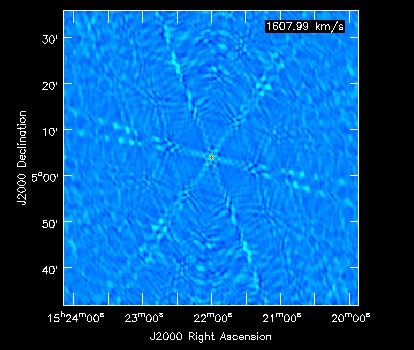

Imaging
                            Principles
          Vij (bij ) = 2D FT{Bprimary.Isource} (bij ) +Noise

• Irregular, limited sampling function:
– S(u, v) = 1 at (u, v) points where visibilities are measured
– S(u, v) = 0 elsewhere
• Bdirty = 2D FT−1 {S}
• Imeas = 2D FT−1 {S.V } → 1) Gridding + FFT to get Imeas

Fourier Transform Property #1:

 Imeas = Bdirty * {Bprimary.Isource} → 2) Deconvolution to get Isource

Bdirty: Point Spread Function (PSF) of the interferometer
(i.e. if the source is a point, then Imeas = Itot.Bdirty).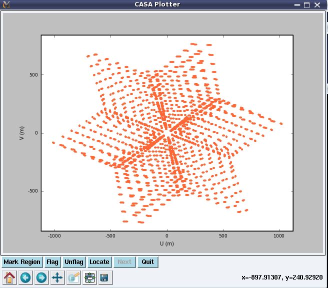

Imaging
                       Principles mapping
• From uv-plane to image plane → build a dirty image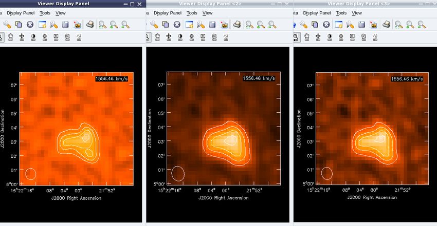

Imaging
                        Principles clean
• From dirty image to clean image (replace the dirty psf by a
cleaned one : without sidelobs)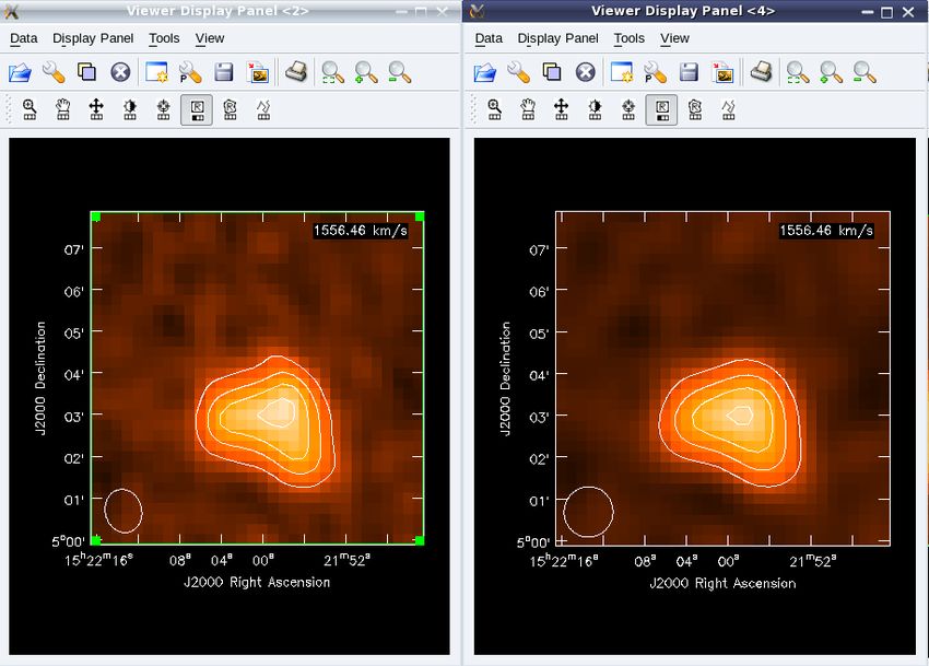

Imaging
                     CASA

• Use the clean() task to both the image and the clean

• To build the dirty image do niter=0 (see later)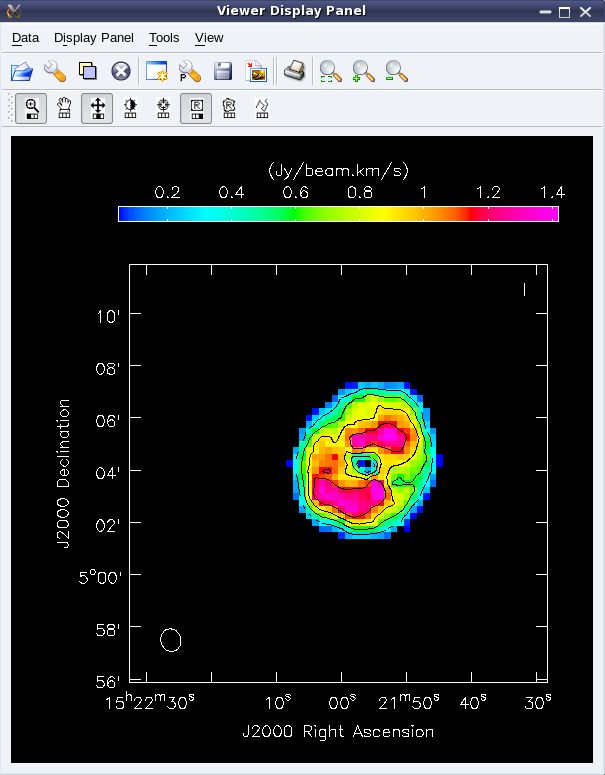

Input / output files

Imaging
                        Dirty map
Spatial Parameters

- Field, scan, antenna, uvrange

Spectral Parameters

- Start with selection parameters
Select a spectral window and some channels with the spw
  parameter spw='0:0~10,1:20~30,2:1;2;3'

- How do I define the final spectral resolution ?
Mode: mfs (continuum), channel or velocity (emission line:
  nchan, start, width ... )

Spatial and Spectral selections

Imaging
                         Dirty map

Spatial Parameters (grid, fft)

- Start with selection parameters
Select a field (calibrator, target) and the stoke parameter (I,IV,
  QU,IQUV) you want to image

- What should be the cell size (sampling) ?
Cell : Between 1/3 and 1/5 of the synthesized beam to ease
  deconvolution

- What should be the map size ?
Imsize: At least twice the primary beam size or more and avoid
  bright sources near the edge of the image that would cause
  aliasing

Mapping parameters

Imaging
                       Clean Image

Cleaning methods
psfmode – algorithm used to calculate the point spread
  function (psf). Hogbom is robsut but slow. Clark is fast
  but unstable (when high sidelobes)

Imagermode ‘csclean’ – similar to ‘clark’ should be used
  for high dynamic range and is always used for mosaics.
  Better accuracy but slow (cf mx in gildas)

Polarization
‘hogbom’ currently only way to clean I, Q, U, & V
  independently. For polarization imaging ‘clark’ searches
  for peak in I2+V2+Q2+U2

Imaging
                               Clean Image

When do I stop cleaning ?
Stop cleaning when the residuals are noise like, and/or the clean has stopped
  converging (adding to cleaned flux)!

niter – Number of clean iterations to do. This can be useful when you are doing
  tests, but this parameter has NO physical meaning. Instead set to large number
  and let either threshold or do interactive to stop the cleaning.
threshold – Stop cleaning when peak residual has this value, give units (i.e. mJy).
  One would like to approach about 3x the theoretical rms noise.

Note:
- To reach this limit the data must be well calibrated/flagged and suffer from no
  serious artifacts (resolved out extended structure/negative bowls, poor psf/uv-
  coverage, dynamic range limited etc).

- Do not set this blindly! Once you reach rms (whether close to theoretical or
  not), you are just picking noise up one place and putting it down in another

Cleaning parameters

Imaging
                       Clean Image

Interactive Cleaning

Interactive Cleaning

Imaging
                               Weighting

• natural – lowest noise, poorest resolution, default
• uniform – highest noise, best resolution
• briggs – intermediate between natural and uniform
      - Default robust=0.0 is often a good choice, range -2 to 2, positive
  more towards natural, negative, more towards uniform
     - npixel number of pixels to determine uv-cell size, default 0 = imsize

Imaging
               Weighting

Uniform        Natural        Robust
2.8 mJy/beam   2.0 mJy/beam   2.0 mJy/beam

Imaging
                                 UV-range

• An image can be dramatically changed by narrowing uv-
  range or applying outer uv-taper

• uvtaper=True
       - outertaper - default unit is meters
      - outertaper=[‘120arcsec’]
      - outertaper=[‘5klambda’,’3klambda’,’45.0deg’]
      - outertaper (klambda) / 200 = outertaper (arcsec) : 5klambda → 25 arcsec
      - Innertaper not yet implemented

Imaging
                                 UV-range

• An image can be dramatically changed by narrowing uv-
range or applying outer uv-taper Outertaper=['60arcsec']

• uvtaper=True
       - outertaper - default unit is meters
      - outertaper=[‘120arcsec’]
      - outertaper=[‘5klambda’,’3klambda’,’45.0deg’]
      - outertaper (klambda) / 200 = outertaper (arcsec) : 5klambda → 25 arcsec
      - Innertaper not yet implemented

                      Increase sensitivity to extended sources

Weighting parameters

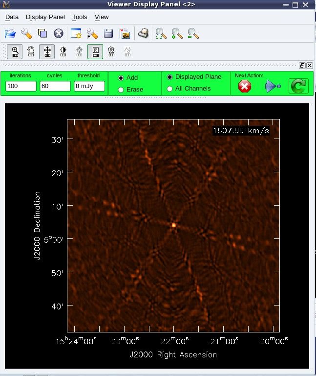
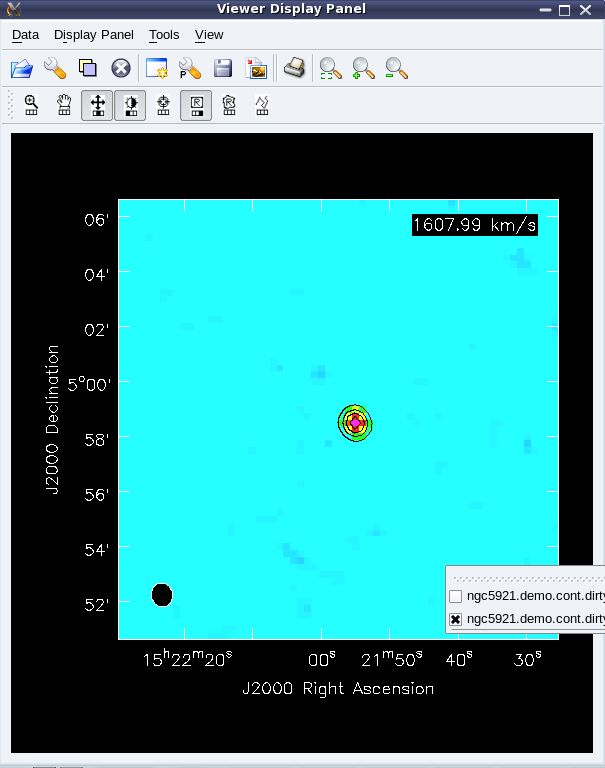
Imaging
                                Output files

Based on the imagename these files are created:

imagename.image – final cleaned (or dirty if niter=0 image)
imagename.psf – the point spread function of the beam, useful to
check whether image artifacts are due to poor psf

imagename.model – an image of the clean components
imagename.residual – the residual image after subtracting clean
components, useful to check if more cleaning is needed
imagename.flux – the primary beam response function – used to make
a “flux correct image”, otherwise flux is only correct at the phase
center(s). pbcor=T divides the .image by the .flux. Such images don’t
look pretty because the noise at the edges are also increased, but
flux densities should ONLY be calculated from pbcor’ed images.

Imaging
                                 Output files

 Based on the imagename these files are created:

 imagename.image – final cleaned (or dirty if niter=0 image)
 imagename.psf – the point spread function of the beam, useful to
 check whether image artifacts are due to poor psf

 imagename.model – an image of the clean components
Use the viewer() to see raster maps, contours...
 imagename.residual – the residual image after subtracting clean
 components, useful to check if more cleaning is needed
 imagename.flux – the primary beam response function – used to make
 a “flux correct image”, otherwise flux is only correct at the phase
 center(s). pbcor=T divides the .image by the .flux. Such images don’t
 look pretty because the noise at the edges are also increased, but
 flux densities should ONLY be calculated from pbcor’ed images.

Imaging
                       Analysis

•   task imhead - get and change image header
    information
•   task immoments - computes moment images of
    spectral cube

•   task imstat - return statistics on regions of image
•   task imval - return values for pixel or region of image
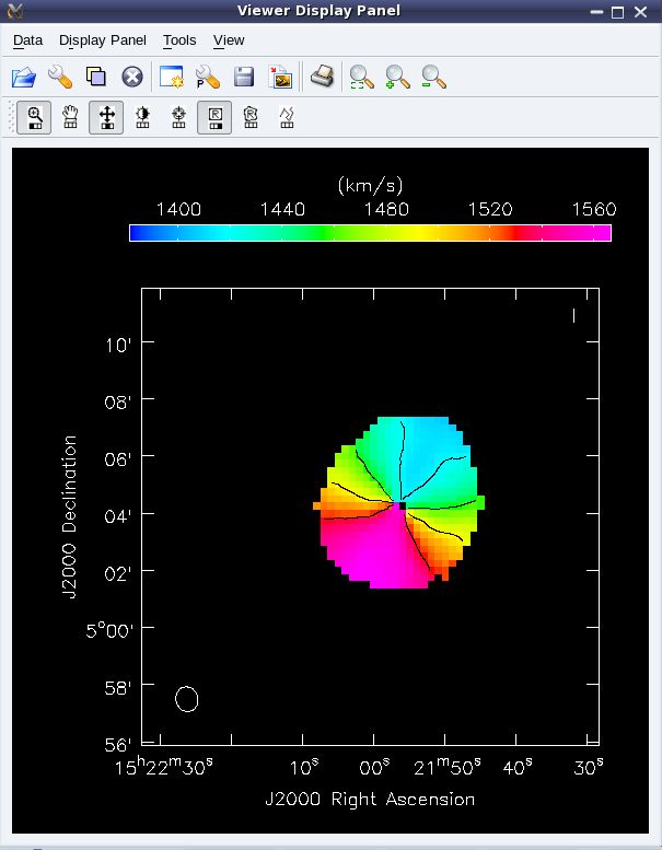
•   task imfit - fit a 2D Gaussian to the image

Imaging
Immoments

Imaging
Immoments

Imaging
                           Large scale

Large scale imaging (mosaic)
Widefield() or clean() with imagermode='mosaic'
Specific methods for ftt, weighting and cleaning of the different
  pointings observed that will make the full final image

Zero/short spacing (extended emission)
feather() – combine a single dish and interferometric image in
  the image-plane. If there is is good overlap in the UV-plane,
  and the relative calibration between the two is accurate this
  should work pretty well

More ...

Exercices
  Go back through the ngc5921_demo.py script

References
   - NRAO Lectures
   http://www.cv.nrao.edu/course/astr534/ERA.shtml
   - IRAM schools (2010 Oct. 4th -8th , Grenoble, France)
   http://www.iram.fr/IRAMFR/IS/school.htm

The end !

Imaging
                        Principles

  From visibilities to images
    Imeas = Bdirty * (Bprim x Isource ) + N

Imeas : Dirty Map
Bdirty : Dirty Beam
Bprim : Primary Beam
Isource : Sky brightness distribution
N : Noise