Interpolation of rainfall for the Albuquerque area : a comparison to the Primary Local Climatological Data Site
←
→
Page content transcription
If your browser does not render page correctly, please read the page content below
University of New Mexico
UNM Digital Repository
Water Resources Professional Project Reports                                                                                      Water Resources

12-17-2013

Interpolation of rainfall for the Albuquerque area : a
comparison to the Primary Local Climatological
Data Site
Christopher N. Wolff

Follow this and additional works at: https://digitalrepository.unm.edu/wr_sp

Recommended Citation
Wolff, Christopher N.. "Interpolation of rainfall for the Albuquerque area : a comparison to the Primary Local Climatological Data
Site." (2013). https://digitalrepository.unm.edu/wr_sp/24

This Technical Report is brought to you for free and open access by the Water Resources at UNM Digital Repository. It has been accepted for inclusion
in Water Resources Professional Project Reports by an authorized administrator of UNM Digital Repository. For more information, please contact
disc@unm.edu.
Interpolation of Rainfall for the Albuquerque Area:
 A comparison to the Primary Local Climatological
                      Station

                               By
                      Christopher N. Wolff

                            Committee:
                           David Gutzler
                           Julie Coonrod
                           Paul Tashjian

    A Professional Project Submitted in Partial Fulfillment of the
                  Requirements for the Degree of
                    Master of Water Resources
                Policy Management Concentration
                     Water Resources Program
                   The University of New Mexico
                     Albuquerque, New Mexico
                           December2013

                                                                     1
Table of Contents

List of Figures                                             3
List of Tables                                              4
Acknowledgements                                            5

Abstract                                                    6

1.0    Introduction                                         7
1.1    Problem Statement                                    8
1.2    Purpose                                              9
1.3    Project Scope                                        9
1.4    Study Location                                       10
1.5    Geographical & Physical Setting                      11
1.6    Climatological Setting                               11
2.0    Monitoring Network                                   12
2.1    Network Descriptions                                 13
3.0    Data Processing                                      17
3.1    Defining Seasons                                     18
4.0    Overview of Geostatistical Interpolation Methods     21
4.1    Empirical Bayesian Kriging (EBK)                     21
4.2    Semivariogram Estimation                             22
4.3    EBK Interpolation Standards                          23
4.4    Analyzing Interpolations                             23
4.5    Sub‐regional Determination                           24
4.6    Sub‐regional Standard Error                          26
5.0    Estimated Annual Precipitation                       27
5.1    StudyNet Estimated Annual Precipitation              30
6.0    Comparison of EAP with LCD measured values           31
6.1    Comparison of StudyNetEAP with LCD measured values   37
6.2    Observable Trends (Interpolations)                   45
7.0    Discussions and Conclusions                          46
8.0    Recommendations and Further Research                 51
9.0    References                                           53
10.0   Appendices                                           57

                                                                 2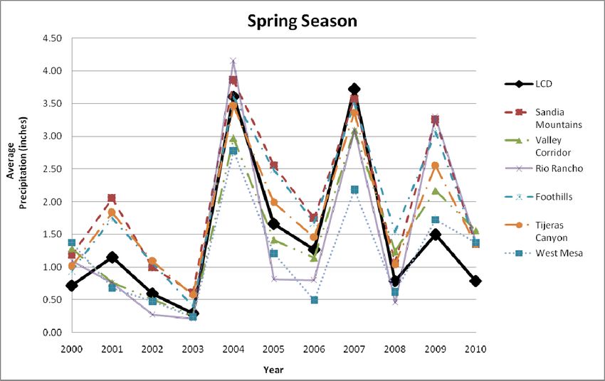
List of Figures
Figure 1 ‐ A map of New Mexico and large cities with large‐scale topography 10
Figure 2 ‐ Regional map and station coverage 17
Figure 3 ‐ NWS Albuquerque Precipitation 30‐year normal comparison 19
Figure 4 ‐ Semivariogram plot 21
Figure 5 ‐ Location analysis map 24
Figure 6 ‐ Difference between Winter Season sub‐regional LCD and EAP 32
Figure 7 ‐ Difference between Spring Season sub‐regional LCD and EAP 34
Figure 8 ‐ Difference between Monsoon Season sub‐regional LCD and EAP 35
Figure 9 ‐ Difference between Water Year Season sub‐regional LCD and EAP 37
Figure 10 ‐ Annual time series of StudyNetEAP and LCD (Winter). 38
Figure 11 ‐ Winter LCD values plotted against corresponding StudyNetEAP 39
Figure 12 ‐ Annual time series of StudyNetEAP and LCD (Spring) 40
Figure 13 ‐ Spring LCD values plotted against corresponding StudyNetEAP 41
Figure 14 ‐ Annual time series of StudyNetEAP and LCD (Monsoon) 42
Figure 15 ‐ Monsoon LCD values potted against corresponding StudyNetEAP 43
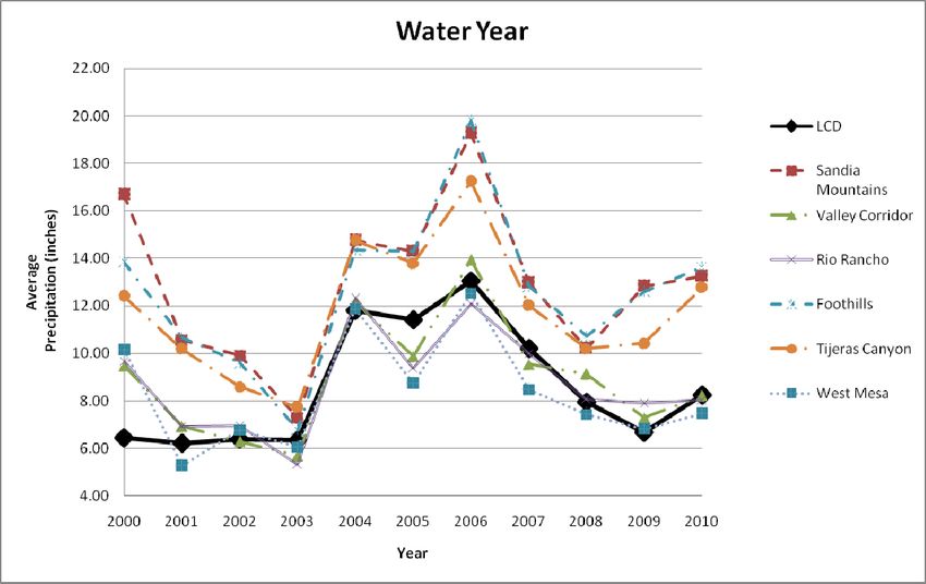
Figure 16 ‐ Annual time series of StudyNetEAP and LCD (Water Year) 44
Figure 17 – Water Year LCD values plotted against corresponding StudyNetEAP 45
3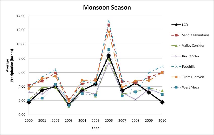
4
List of Tables

Table 1 ‐ Codified semivariogram interpolation parameters                22

Table 2 ‐ Winter Season sub‐regional EAP calculation                     28

Table 3 ‐ Spring Season sub‐regional EAP calculation                     28

Table 4 ‐ Monsoon Season sub‐regional EAP calculation                    29

Table 5 ‐ Water Year sub‐regional EAP calculation                    .   29

Table 6 ‐ Winter Season StudyNet EAP Calculation (00‐10)                 30

Table 7 ‐ Spring Season StudyNet EAP Calculation (00‐10)                 30

Table 8 ‐ Monsoon Season StudyNet EAP Calculation (00‐10)                31

Table 9 ‐ Water Year StudyNet EAP Calculation (00‐10)                    31

Table 10 ‐ Difference between Winter sub‐regional EAP and the LCD.       32

Table 11 ‐ Difference between Spring sub‐regional EAP and the LCD.       33

Table 12 ‐ Difference between Monsoon sub‐regional EAP and the LCD       35

Table 13 ‐ Difference between Water Year EAP and the LCD                 36

Table 14 ‐ Difference between Winter StudyNetEAP and the LCD             38

Table 15 ‐ Difference between Spring StudyNetEAP and the LCD             40

Table 16 ‐ Difference between Monsoon StudyNetEAP and the LCD            42

Table 17 ‐ Difference between Water Year StudyNetEAP and the LCD         44

                                                                              5
Table 18 – Factor differences between LCD annual precipitation and EAP                      49

Acknowledgements

       First I would like to thank my family for their uncompromising support and for instilling
in me the drive and passion to learn.

       To my wonderful girlfriend, who told me to always pursue a career and a degree that
allows me to make a difference in the world and for our environment. Thank you for your
patience and love.

       I would also like to thank Dr. David Gutzler (Committee Chair) for his support and
guidance throughout the development and realization of my professional project. This project
would not be what it is without his brilliance and leadership.

Thank you to Julie Coonrod (Committee Member) for helping me discover how useful GIS can be
to analyze aspects of Water Management. Also thank you for being a great professor.

Thank you to Paul Tashjian (Committee Member) for your help, your friendship, and for bringing
me into the Fish and Wildlife Service family. Working for you guys at FWS was the best job I
have ever had. Also, a warm thanks to the FWS Region 2 Water Resource Team for being great
gentlemen of the Federal Service.

Special thanks to Dr. Deirdre Kann and the National Weather Service Team in Albuquerque.
Without your insight, direction and data this project would not have seen the light of day.

Thanks to Bruce Thomson for his leadership as Director of the Water Resources Program and
for bringing me to UNM and allowing me to join the WRP graduates.

                                                                                                   6
Finally thank you to all the UNM professors, staff, and students which I had the pleasure to
meet and work with during my time at UNM. You made my graduate experience dynamic and
exciting.
Abstract
The main objective of this project was to assess the ability of the Primary Local
Climatological Data Site (LCD) to estimate precipitation around the City of Albuquerque. In
other words, this study determined how representative LCD precipitation data is as a point
source station for characterizing precipitation within the Albuquerque metro area and nearby
sites. Because the LCD is located in a permanent position near the Albuquerque International
Airport, precipitation associated with rainfall localized away from the LCD, but within the
Albuquerque metro area, is not accounted for in the LCD precipitation data record. This study
quantified regional variability in rainfall that cannot be captured by any single station by
combining three primary source precipitation programs into a single comprehensive
precipitation monitoring network (StudyNet) for the study period 2000 – 2010.
Sub‐regions within the StudyNet Region were identified and subjectively demarcated to
include variations in topography, elevation, predominant wind and weather patterns, and areas
with higher and lower densities of monitoring stations. Estimated Annual Precipitation (EAP)
was determined by evaluating the results from objective seasonal spatial interpolations. Using
estimated precipitation range for each interpolation, displayed by color scales, minimum and
maximum precipitation levels were assigned for each sub‐region. Maximum and minimum
estimated precipitation values associated with each sub‐region were then averaged to
determine the EAP for each sub‐region. For additional analysis, sub‐regional EAP results were
summed and averaged for each year to determine the StudyNet Estimated Annual Precipitation
(StudyNetEAP).
As results show, the LCD values were closest to spatially averaged precipitation in the
Spring Season precipitation with a strong positive Pearson correlation of .95 and the lowest
root mean squared difference (.40) in the Spring. Winter Season precipitation was
underestimated by the LCD 64% of the time and had a moderately positive correlation
7coefficient (.72). During wet periods, especially the monsoon season when convective
precipitation patterns display high spatial variability, the LCD frequently underestimates yearly
precipitation, 90% of the time, with an average underestimation of 4.82 in/yr. Water Year
precipitation was shown to have the highest root mean squared difference (2.09) and had a
strong positive Pearson’s correlation of .87 between LCD and StudyNetEAP values.
Quantifying seasonal precipitation shows that the LCD systematically underestimated
StudyNetEAP in every season, and also in the annual mean. During dry periods the LCD was
better at capturing both sub‐regional and StudyNet wide precipitation. During times of
sporadic and intense storm events the LCD often missed sub‐regional precipitation events and
consistently underestimated total precipitation for the StudyNet region. However, when LCD
measurements are adjusted by sub‐regional factor differences, the constant bias is removed.
After removing the sub‐regional bias the LCD measurement can be used to estimate seasonal
sub‐regional precipitation and thus regional precipitation for the greater Albuquerque area.
Additionally, high seasonal correlations between LCD precipitation and StudyNetEAP show that
the LCD provides a useful metric for determining dry and wet years for the StudyNet region as a
whole
1.0 Introduction
Proper characterization of precipitation events can provide local and regional decision
makers crucial insight for issues regarding water management, infrastructure planning, and
erosion control. Yet tracking their frequency, distribution and rainfall totals associated with
these events can be difficult due to a lack of monitoring stations, difficult topography, or due to
the infrequent and sporadic nature of precipitation. Monitoring precipitation along the
Albuquerque landscape is no different. The topography of the Albuquerque area can
dramatically affect the amount, frequency, and distribution of precipitation across the city and
region (Leopold 1951).
This study looks to determine the temporal and spatial variability of precipitation across
the Albuquerque region for an 11 year period (2000‐2010), during which a comprehensive
8network of precipitation stations (denoted the StudyNet) is assembled from separate data
sources. An objective spatial interpolation technique is used to produce a surface gridded
precipitation product that spans the Albuquerque metro area. From precipitation
interpolations, values of sub‐regional Estimated Annual Precipitation (EAP) and StudyNet
Estimated Annual Precipitation (StudyNetEAP) across the entire area, are derived. From these
estimations, seasonal, yearly, sub‐regional and regional trends are analyzed and results are
compared to the precipitation variability measured at the Primary Local Climatological Data Site
(LCD) adjacent to the National Weather Service Office at the Albuquerque International Airport.
1.1 Problem Statement
With the 10,687 ft. Sandia Mountains rising to the East, the dormant Vulcan Volcano
approximately 6000 feet above sea level to the West, and a Valley floor near 4900 ft, the
topography of Albuquerque, New Mexico is dramatic (City 2013). East‐west topographic
gradients are extreme: the top of Vulcan Volcano is only about 20 miles away from the top of
the Sandia Mountains, with the Rio Grande in between. Mountainous areas often receive more
precipitation than the basin floors due to orographic effects (Guan et al. 2005). Large variations
in topographic relief can be a major force driving local weather patterns and have the ability to
enhance the erratic behavior of localized storm events (Sotillo et al. 2003).
Precipitation events around the Albuquerque metropolitan area are often spatially and
temporally distributed due to these large variations in topography. During the monsoon season
(July – August) precipitation events can occur in flashy and intermittent patterns (WRCC 2013).
And though rain can be observed in downtown Albuquerque, the University of New Mexico,
approximately two miles away may receive no rainfall. During the winter months higher
precipitation accumulations are observed in the Sandia Mountains, than are observed in the
rest of the Albuquerque area, but with notable differences over the west versus east slopes
(WRCC 2013). Additionally, precipitation events can vary dramatically from season to season
and year to year due to interannually varying weather patterns and other factors associated
with seasonal precipitation (WRCC 2013).
9The Primary Local Climatological Data Site (LCD) for the Albuquerque area is
administered by the National Weather Service (NWS, a division of the National Oceanic and
Atmospheric Administration or NOAA) Forecast Office, located at the Albuquerque
International Airport (often called the Sunport). The LCD is located at an elevation of 5,308 feet
above sea level on a flat exposed area southeast of downtown Albuquerque (NOAA 2012). The
LCD is the principal climatological data collection site used by NOAA to analyze precipitation
totals for Albuquerque (NOAA 2012). In addition to the LCD, the NWS Albuquerque Forecast
Office routinely uses three other sites around Albuquerque for localized monitoring and
forecasting purposes. Using data collected at these sites specific forecasts are made for those
areas. With the variable frequency of storm patterns, the temporal distribution of rainfall
events, and dramatic elevation differences, the Albuquerque region contains distinct
microclimates. Precipitation events occurring away from the Sunport, but within the
Albuquerque metro area, may not be captured by the LCD measurement.
1.2 Purpose
The purpose of this study is to quantify, through the objective interpolation of rainfall
data, how accurately the LCD precipitation record(2000 – 2010) characterizes seasonally
averaged precipitation and its interannual variability for the broader Albuquerque study area.
This analysis will quantify regional variability in rainfall that cannot be captured by a single
station. The results of this study may provide a greater understanding of: whether regional
precipitation gauges would provide a more accurate assessment of climatological precipitation
than a single location; identify spatial trends associated with precipitation in the identification
of a systematic bias; quantify the degree to which precipitation is under or overestimated for
the Albuquerque region by utilizing the single station approach; and other temporal or spatial
precipitation patterns associated with the study period. Through quantitative analysis of
spatially interpolated rainfall data, derived from an extensive network of in situ precipitation
gauges assembled for this study, the ability of the LCD to estimate sub‐regional and regional
precipitation is assessed.
101.3 Project Scope
This project combined precipitation data
collected from three separate rainfall monitoring
programs located in and around the Albuquerque
area. The merging of these various data sources
into a single comprehensive network represents a
useful and significant research product derived from
this study. This accumulated study network (StudyNet) is comprised of NWS COOP Stations
(NWS 2013), Community Collaborative Rain Hail and Snowfall Network (CoCoRaHS) stations,
(CoCoRaHS 2013) and Albuquerque City Net (Kann 2013) locations. The merged data set
provided anchor points for seasonal analysis using ArcGIS
Figure 1 ‐ A map of New Mexico indicating
10.1 Geostatistical Analysis Interpolation (ESRI 2013). location of large cities (including Albuquerque)
and large‐scale topography (green)
The Albuquerque Region was defined after
analyzing the distribution of the StudyNet station locations and incorporates approximately 600
square miles. Sub‐regions are subjectively identified and delineated to account for variations in
topography, elevation, predominant wind and weather patterns, and areas with higher and
lower densities of monitoring stations. Though weather patterns associated with orographic
gradients and other topographically driven weather patterns are observed in this analysis,
elevation is not a covariate accounted for in the interpolation, unlike some other statistical
interpolation methods such as that developed by the PRISM Climate Group (Daly 2008).
1.4 Study Location
The City of Albuquerque, and surrounding metropolitan area, is located near the center
of the state of New Mexico (Figure 1). In 2010, the city of Albuquerque’s population was
11545,852 (U.S. Census Bureau, 2010) having grown from 243,751 in 1970 (U.S. Census Bureau,
1973). Furthermore, this boom in population growth reflects an increasing devotion to urban
development and urban sprawl. A 1997 U.S. Geological Survey study mapped urban land use
from aerial photographs and noted that the Albuquerque metropolitan area had grown from
49,746 acres to 84,889 acres between 1973 and 1991, a 71 percent increase in urbanized area
(Braun et. al. 1998). Urban expansion is expected to continue to put pressures on the area's
water resources and flood control systems (Siemers, 2007).
1.5 Geographical & Physical Setting
The Albuquerque metropolitan area is situated in a valley known as the Rio Grande Rift.
Formed by faulting and crustal thinning, the rift has caused a dramatic variation in elevation
profiles for the Albuquerque region (Kelley 2012). Most of the population of the Albuquerque
metro area lives within the confines of the western mesas and the eastern piedmont slopes
rising from either side of the valley floor. From the western edge of the study area, at an
approximate elevation of 6,033 ft above sea level, the elevation drops to the southward flowing
Rio Grande at approximately 4,900 feet. From the valley, the topography gently rises eastward
toward the Sandia foothills to an elevation of approximately 7,000 feet, then abruptly slopes
upward to the top of the Sandia Mountains, soaring above 10,000 feet (Anderson 1961).
1.6 Climatological Setting
The climate of Albuquerque is arid with abundant sunshine, low humidity, scant
precipitation, and a wide seasonal range of temperatures (U.S. EPA 2003). During the summer,
rains fall almost entirely during intense thunderstorms where a southeasterly circulation pulls
moisture from the Gulf of Mexico and Gulf of California into the State (Guido 2013). July and
August are the rainiest months over most of the State, with 30 to 40 percent of the year's total
moisture falling during that time (WRCC 2013). Thunderstorm frequency typically increases
rapidly around July 1st, peaks in August, and then tapers off by the end of September. Summer
12thunderstorms are usually brief but have the ability to produce heavy rainfall in localized areas.
Winter is the driest season in New Mexico (WRCC 2013). While the mountains can receive
substantial snowfall during the winter months, winter storms deliver precipitation as either rain
or snow to the valleys (WRCC 2013).
Temperatures in Albuquerque are characteristic of a dry, high desert climate (WRCC
2013). Within the Albuquerque basin elevation and proximity to the Rio Grande can be key
factors in determining local temperatures. Average monthly maximum temperatures during
July, the warmest month, range from 90° F at lower elevations to the upper 70's at higher
elevations. In the summer, individual daytime temperatures in Albuquerque can exceed 100° F.
Additionally, there are large diurnal fluctuations in temperatures during the summer and fall
seasons. On average, high temperatures during the winter hover around 50°F. Mean annual
temperature ranges from 57°F at the Albuquerque Airport to 38°F at Sandia Crest, a difference
in elevation of5,365 feet. Sustained winds of 12 mph or less occur approximately 80 percent of
the time at the Albuquerque International Airport, while sustained winds greater than 25 mph
have a frequency less than 3 percent. Late winter and spring weather systems along with
occasional easterly winds out of Tijeras Canyon are the primary sources of strong wind
conditions. While east winds events are the more dominant type of high wind event on an
annual basis, late winter and spring wind events are associated almost equally with both east
(gap wind) events and systems with a westerly component (Shoemake 2010).Blowing dust
often accompanies the occasional strong winds in winter and spring seasons (NOAA 2013).
2.0 Monitoring Network
Precipitation collected using rain gauges are point source data by definition. Thus total
rainfall data for an area must be estimated through various means. For this study, point source
rainfall data were analyzed to produce a gridded product using objective spatial interpolation
methods. The accuracy and representation of rain fall data is controlled by the spatial
distribution of the weather stations and by the interpolation method used. Since the
distribution of monitoring stations and the interpolation method have such a large effect on the
13rainfall estimations, results may or may not reflect the actual spatial pattern of rainfall for any
given event. For this reason, we sought to expand the spatial coverage and density of
precipitation data across the Albuquerque region by combining gauge data from three separate
primary sources. Combining these data sources provide a comprehensive gauge network for
the StudyNet Region.
These networks are the Community Collaborative Rain, Hail, and Snow Network
(CoCoRaHS 2013), the National Weather Service Cooperative Observer Program (NWS 2013),
and Albuquerque City Net weather monitoring program (Kann 2013). Each of these volunteer
based networks utilizes similar gauge standards and precipitation monitoring protocols as
described in detail below.
2.1 Network Descriptions
A. Community Collaborative Rain, Hail and Snow Network (CoCoRaHS)
The Community Collaborative Rain, Hail and Snow (CoCoRaHS) Network is a community
based network of volunteers who take daily measurements of rain, hail and snow in their
backyards (CoCoRaHS 2013). It was created to enhance the accuracy of precipitation mapping
and for reports intense storms. The CoCoRaHS program came about as a result of a devastating
flash flood that hit Fort Collins, CO in 1997 when a very localized storm dumped over a foot of
rain in some areas of the city while other portions of the city had only modest rainfall
(CoCoRaHS 2013). Events like these occur across the country, including in Albuquerque, and
are the purpose for the program. CoCoRaHS data now extend over a period of time of
sufficient length to provide useful climatic data that can be used by scientists and researchers
to study multi‐year climate variability in addition to studies of individual weather events.
The CoCoRaHS website describes the only requirements to participate in the CoCoRaHS
program is to have “an enthusiasm for watching and reporting weather conditions and a desire
to learn more about how weather can effect and impact our lives”. As rain, hail or snow events
cross an observation area, volunteers take measurements of precipitation from as many
14locations as possible. These precipitation reports are then recorded on the CoCoRaHS web site.
The data are then displayed and organized online for end users (CoCoRaHS 2013).
Measuring:
CoCoRaHS has developed protocols for gathering and reporting data. As described by
the CoCoRaHS website, gauges should be placed in an area that is protected from strong winds
but not bothered by obstacles that could either block precipitation from reaching the gauge or
cause precipitation to splash towards it. The gauge should be installed 2‐5 feet above the
ground mounted on the side of a single post. The top of the rain gauge should extend several
inches above the top of the mounting post and the mounting post should have a rounded,
pointed, or slanted top to avoid upward splash towards the rain gauge (CoCoRaHS 2013). For
more on CoCoRaHS procedures can be found in the measuring rain section of the CoCoRaHS
website.
Reporting:
Each CoCoRaHS report includes the volunteer name, station number, station name, time
rain gauge was measured, and the amount of precipitation that has fallen within the past 24
hours. Estimated rainfall amounts are recorded by observers, then the reports are uploaded by
CoCoRaHS staff to the CoCoRaHS website. Trace rainfall, as described on the CoCoRaHS
website as “precipitation that is seen or felt that is not a measurable amount”, is recorded by
observers but reported as 0.00 inches even if there are multiple days with trace rainfall.
B. National Weather Service Cooperative Observer Program (COOP)
The NWS describes the Cooperative Observer Program (COOP) as the “Nation's weather
and climate observing network” (NWS 2013). More than 11,000 volunteers take observations
on “farms, in urban and suburban areas, National Parks, seashores, and mountaintops. Formally
created in 1890, the mission of the COOP program is: (1) providing observational
meteorological data, usually consisting of daily maximum and minimum temperatures,
15snowfall, and 24‐hour precipitation totals, required to define the climate of the United States
and to help measure long‐term climate changes, (2) providing observational meteorological
data in near real‐time to support forecast, warning and other public service programs of the
NWS (NWS 2013). The NWS COOP program helps volunteers and partners train observers,
select optimal monitoring sites, install and maintain equipment, collect and deliver data, and
maintain data and quality control. A cooperative station is a site where rainfall observations
are taken by volunteers or contractors. Automated observing stations are considered
cooperative stations if their observed data are used for services which otherwise would be
provided by cooperative observers. A cooperative station may be collocated with other types
of observing stations such as standard observations stations, Flight Service Stations, etc. In
these cases, that portion of the station observing program supporting the cooperative
program's mission is treated and documented independently of the other observational and
service programs.
Measuring:
Observers generally record temperature and precipitation daily and electronically send
those reports daily to the NWS and the NOAA National Climatic Data Center (NCDC). Many
cooperative observers provide additional hydrological or meteorological data, such as
evaporation or soil temperature. Data are transmitted via telephone, computer or, in special
cases, by mail. Equipment used at NWS cooperative stations may be owned by the NWS, the
observer, or by a company or other government agency, as long as it meets NWS equipment
standards. In order to preserve the integrity of the network, NWS has established standards for
equipment, setting, and exposure. Gauges, similar to the CoCoRaHS standards, are not to be
located close to obstructions which may deflect or alter precipitation due to turbulence.
Additionally the COOP program website recommends that gauges should not to be located in
open spaces or on elevated sites, because of resulting turbulence from the wind (NWS 2013).
Reporting:
16Although the majority of cooperative stations record precipitation amounts and
maximum and minimum temperatures, the COOP program describes each station as unique.
For example, one station may record precipitation only, while another station may record
precipitation, temperature, and evaporation. Measurements, as described by COOP Program
protocols, are taken and recorded daily of the amount of rainfall, snowfall (new snow), depth of
snow, and for other forms of precipitation. Records are kept of the character, type, and time of
occurrence. Each station is typically furnished with a non‐recording or a weighing‐type
recording gauge and when a new station is established, the NWS representative trains the
volunteer observer in the established weather observation, recording, and the station
maintenance techniques (NWS 2013). Observations taken any time between 6am and 8am are
usually acceptable if coordinated and approved by the NWS but all observations are required to
be taken at the same time every day throughout the year (NWS 2013).
C. National Weather Service CityNet (CityNet)
Precipitation monitoring stations in this network, similar to the CoCoRaHS Network and
NWS COOP Observer Program, are managed by volunteers around the Albuquerque Metro
area. CityNet data are gathered and compiled by staff at the NWS Albuquerque Weather
Forecast Office (WFO) in the form of Excel spreadsheets. Daily observation data were
organized into monthly data by NWS staff and similar recording and data compliance protocols
are followed as standardized by the NWS COOP program as described above (Kann 2013).
D. Study Network (StudyNet)
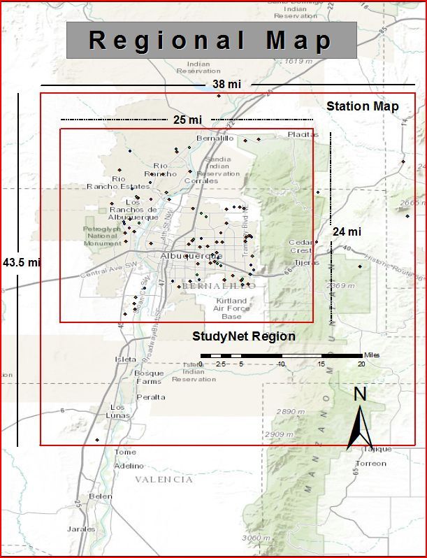
Using longitudinal and latitudinal coordinates for each precipitation station, a
geographic information system (GIS) station coverage map was created. From this map a Study
Network (StudyNet) was delineated based upon overall station coverage and defined to include
important topographical characteristics associated with local precipitation patterns. In total the
17study area covers approximately 600 square miles and extends 25 miles east west by 24 miles
north o south (Figure 2).
Additionally, other stations within 20 miles of the StudyNet boundary were included, to
assure greater accuracy in the interpolation process and to limit the standard error associated
with the interpolations. Due to the volunteer nature of the monitoring programs and overall
mobility of individuals in such programs, the number of stations in the StudyNet region varies
from year to year. Station variability
is taken into account though the EBK
interpolation (Krivoruchko 2012).
The StudyNet region within the
Station Map is the delineated area
where interpolations are performed
(Figure 2).
3.0 Data Processing
Daily precipitation values
were compiled from the three
separate networks. The data were
combined and processed using an
Excel spread sheet pivot table to sum
the daily precipitation data into
monthly time series of total
precipitation for each individual
gauge site. Latitudes and longitudes for each station were compiled for use in the interpolation
analysis. Stations lacking an identification number were assigned one to maintain a consistent
numerical order. To be included in the StudyNet data set, monitoring stations must have
had a minimum of 6 months of rainfall data per year. This minimum standard did not remove
individual stations from the overall interpolation, because once a station reached the 6 month
18
Figure 2 ‐ Regional map and station coverage map with StudyNet study area
delineated by red rectangles. Inset within the StudyNet region is the City of
Albuquerque, NM (beige) with Sandia and Manzano Mountains (green)data standard it was included in the subsequent interpolation. An average of two stations
lacking 6 months of data were identified per year within the StudyNet region and removed
from the analysis table until the 6 month standard was met.
Stations must have been actively recording precipitation for at least 5 of the 11 years to
be included in the analysis. Only four stations were excluded from the interpolation as they
lacked the minimum 5 years of data. Exclusion of such outliers could potentially have affected
seasonal precipitation totals (ESRI 2013). However, outlier exclusion was found to have little
effect on the overall results of the interpolations. Data associated with stations enrolled in two
or more monitoring networks were averaged as a single station total. Trace rainfall data
(rainfall less than .01 in.) were recorded as 0 within the analysis table to conform with NWS
standards (NWS 2012). Stations missing data, but in conformance with the minimum data
standards, were intentionally left blank (not recorded as zero), to assure the data were not
skewed toward a lower seasonal or yearly average. Snow data were excluded from the analysis
due to the inconsistency of observed measurement by volunteers, variability in snow type, and
unknown methods by which volunteers may have derived the liquid water equivalent of snow.
The exclusion of snow data could possibly lead to an underestimation of precipitation totals,
especially during the Winter Season and in Sandia Mountains and Foothills sub‐regions.
However, with less than one third of total stations collecting snow data, ambiguity in
measurement techniques and by excluding snow data region wide, results of this study are not
affected in a significant manner.
3.1 Defining Seasons
It is important to define seasons in the StudyNet region because different weather
phenomenon and thus different precipitation patterns vary significantly during the year.
Meteorological seasons, tailored to match the climate of the Albuquerque region, were defined
for this study. Analyzing data over seasonal time periods allows this study to capture both
individual storm events and region wide events associated with seasonal weather patterns.
Analyzing data from individual events, as CoCoRaHS data is designed to do, would draw
19conclusions to the ability of the LCD to
characterize single, often localized storm
events. As the LCD is stationary and
precipitation falling across the study
region is spatially heterogeneous,
especially during the Monsoon Season, it
is known that the LCD cannot capture
every precipitation event. Analyzing
interannual precipitation helps draw big Figure 3 – Albuquerque monthly precipitation 30 year normal
comparison indicating the variability of seasonal precipitation
picture conclusions to the LCD’s ability to occurring in the Albuquerque area. 1981‐2010 (dark blue). 1971 –
2000 (light blue).
characterize regional and sub‐regional
precipitation for the greater Albuquerque area. Additionally, assessing interannual variability
of precipitation across seasons provides this study the chance to evaluate the LCD’s ability to
characterize precipitation during wetter than normal Monsoon Seasons and drier than normal
Spring Seasons. Albuquerque monthly precipitation 30‐year Normal’s (1971‐2000 and 1981‐
2010 ) helps to display seasonal differences in average precipitation totals for the study region
(Figure 3).
A. Winter Season (October – March)
The Winter Season time period is extended to six months to include weather
phenomena associated with fall and early spring cycles because the Winter Season, on average,
is the driest season in New Mexico (WRCC 2013). Additionally, cold season storms tend to drop
precipitation over a relatively broad area. During these months, temperatures can drop low
enough to allow precipitation to fall as snow at higher elevations or as either rain or snow at in
lower elevations. Capturing rainfall events and not snowfall events is critical for this analysis.
Extending the Winter Season beyond a more conventional definition allows this study to
capture broader precipitation events, and events associated with late monsoon or early spring
convection systems, as part of a lengthy cold season.
20B. Spring Season (April – June)
From April to June, sporadic thunderstorms occur and high wind conditions can persist
in the StudyNet region. Relatively strong wind events can accompany frontal activity during
late winter and spring periods, and sometimes occur just in advance of thunderstorms (WRCC
2013). A Spring season, defined as April – June, captures late winter events, Spring
thunderstorms, and rainfall associated with an early onset of the summer monsoon.
C. Monsoon Season (July – September)
July and August are the rainiest months in New Mexico (WRCC 2013). Monsoon season
in New Mexico typically begins in early July (WRCC 2013). Summer thunderstorms events can
drop several inches of rain in a localized area in a short time, whereas cold season storms tend
to drop precipitation over a broader area. By analyzing precipitation totals from localized storm
events during the Monsoon Season, this study can draw conclusions to the ability of the LCD to
characterize warm season localized thunderstorm events within the StudyNet area.
D. Water Year (October – September)
Following United States Geological Service (USGS) guidelines for surface water supply, a
water year for this analysis was defined as the “12‐ month period October 1, for any given year
through September 30, of the following year (USGS 2013). By following USGS water year
guidelines, past and future water year data can be utilized in subsequent analyses. Most
importantly, non‐seasonal precipitation totals can be compared to yearly precipitation totals of
the LCD. For this analysis a Water Year is identified using its second calendar year, e.g. Water
Year 2005 refers to the twelve month period Oct 2004 ‐ Sept. 2005.Separate interpolations
were performed utilizing Water Year precipitation data, as opposed summing the three seasons
(Winter, Spring, Monsoon) into a Water Year. The longer time scale (October – September)
21used to assess Water Year precipitation decreases
potential error associated with the smaller seasonal
time‐scale data sets.
4.0 Overview of Geostatistical Interpolation
Methods
It is impossible to collect precipitation data at
every point across a landscape; this is especially true over large areas and in remote locations.
To do so an immense network of monitoring stations Figure 4 – Hypothetical semivariogram plot showing
an example of how estimating semivariograms create
would need to be installed and actively maintained, a distributed average
which would be both economically and physically impossible. Geostatistical tools have been
developed to predict, or spatially interpolate, values at locations between point source data
sites. There are two principal methods for interpolating spatially distributed data: (1)
deterministic (2) probabilistic. Deterministic methods use predefined functions of the distance
between observation locations and the location for which interpolation is required.
Probabilistic methods, the technique utilized in Empirical Bayesian Kriging (EBK) interpolation
and in this study, use statistical theory to quantify the uncertainty associated with interpolated
values (Krivoruchko 2012). Using the ArcGIS Geostatistical EBK tool, and collected data, this
analysis looks to predict, or interpolate, precipitation values across the StudyNet region.
4.1 Empirical Bayesian Kriging (EBK)
The Economic and Social Research Institute (ESRI) describes EBK as “a geostatistical
interpolation method that automates the most difficult aspects of building a valid kriging
model” (ESRI 2013). Other kriging methods in Geostatistical Analyst require a user to adjust
parameters manually in order to obtain accurate results, but EBK automatically calculates these
parameters through a process of subsetting and simulation (ESRI 2013). EBK differs from
classical kriging methods by explicitly accounting for potential error introduced by estimating
22the semivariogram model. This is done by estimating many semivariogram models rather than
a single semivariogram. Semivariograms provide quantitative estimates of the spatial
correlation between observations measured at
specified locations (ESRI 2013). These correlations, Input Datasets
Output Type Prediction
commonly represented on a graph, show the variance
Subset Size 100
in measurements with distance between all pairs of Overlap Factor 1
sampled locations (Figure 4). Semivariogram Number of Simulations 100
Sector Type 4
modeling estimates relationships of point source data
Searching Neighbor Std. Circular
and indicates the variability of the measurements Maximum # Neighbors 15
within a prescribed range. Minimum # Neighbors 10
4.2 Semivariogram Estimation
Table 1‐ Codified semivariogram parameters
Listed below are the steps used in EBK to create used in each interpolation.
semivariograms:
1. A semivariogram model is estimated from annual rainfall data collected from spatially
distributed precipitation monitoring stations.
2. An interpolated value is estimated at each of the input data locations from the
semivariogram.
3. The new semivariogram model is estimated from the simulated data and a weight for
this semivariogram is then calculated showing how likely the observed data can be generated
from the semivariogram.
Steps 2 and 3 are repeated and with each repetition, the semivariogram estimated in
step 1 is used to simulate a new set of values at the input locations. The simulated data are
used to estimate a new semivariogram model and its weight. Predictions and prediction
standard errors are then produced at the unsampled locations using these weights. This
23process creates a wide range of semivariograms, each of which is an estimate of the true
semivariogram from which the compiled data could be generated (Krivoruchko 2012).
Additionally, EBK can be used to interpolate non‐stationary data. The EBK model, in the
case of non‐stationary datasets, first divides point data into subsets of a user specified size
which may or may not overlap. In each subset, distributions of the semivariograms are
produced and for each location a prediction is generated using a semivariogram distribution
from one or more subsets. Each data subset uses models defined by nearby values, rather than
being influenced by very distant factors, yet when all the models are combined, they create a
complete picture (Krivoruchko 2012).
Five other interpolation methods were evaluated for use in this study, including Inverse
Distance Weighted, and Natural Neighbor. These interpolations used similar processing
methods as EBK. However, automating each interpolation method for variable data inclusion
and overall stationarity of the data sites proved difficult for use with this data set. EBK was
chosen for this analysis because it provides an uncomplicated and dynamic method of data
interpolation, requires minimal user modeling, reduces standard error associated with the data,
allows more accurate prediction than other kriging methods and yields a more accurate
interpolation compared to other methods for medium to small datasets.
4.3 EBK Interpolation Standards
To ensure consistent data processing and to establish a codified method for the EBK
interpolation to follow, semivariogram parameters were standardized for each simulation
(Table 1). The EBK method search radius was adjusted on a case‐by‐case basis to ensure that a
minimum of 10 stations and a maximum of 15 stations were used in each interpolation to
mitigate issues associated with non‐stationarity of the monitoring locations.
4.4 Analyzing Interpolations
The EBK interpolation methods are standardized across each year and each season, but
precipitation totals shown in the maps are not equally weighted. The nature of Albuquerque’s
24weather and variability of precipitation during the
seasons makes the standardization precipitation
range difficult. If a standardized color scheme were
designated for precipitation, estimated values would
be indistinguishable in the interpolation maps. By
standardizing the interpolation color patterns and not
precipitation totals, interpolations can still be used to
analyze seasonal rainfall patterns, quantify variability
in rainfall amounts, and provide a comparison of sub‐
regional precipitation to the LCD.
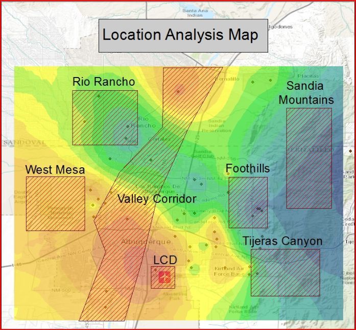
4.5 Sub‐regional Determination
Sub‐regions were demarcated within the StudyNet area to facilitate comparison with
precipitation measured at the LCD. These sub‐regions were subjectively chosen to incorporate
topographical differences within the StudyNet area, station density, and primary weather
corridors. These sub‐regions are: Rio Rancho, West Mesa, Valley Corridor, LCD, Tijeras Canyon,
Foothills, and Sandia Mountains (Figure 5). Features of these sub‐regions are described below.
Figure 5 – Map of StudyNet sub‐regions showing an
example of color scale interpolation. Sub‐regions were
A. Primary Local Climatological Data Site (LCD) delineated to assess the ability of the LCD to estimate
rainfall occurring at a sub‐regional level. Colors display
annual precipitation levels as estimated by seasonal
interpolations (red‐ lowest; dark blue‐highest). Precipitation
The LCD is located at the Albuquerque amounts and associated color ranges are not standardized
across interpolations. Maps are assessed on a yearly and
International Airport and consists of three separate seasonal basis (Appendix A).
precipitation stations averaged as a single station for
this analysis. Located at an elevation of 5,308 feet above sea level (ASL), the LCD is the
principal climatological data collection site NOAA uses to analyze precipitation totals for
Albuquerque area.
B. Rio Rancho (RR)
25Located at an approximate elevation of 5,282 feet ASL, Rio Rancho has experienced
extensive urbanization. With consistent station coverage over the study period, this sub‐region
is a key location to monitor variations in precipitation along the Northwest section of the study
area (Albuquerque 2013).
C. West Mesa (WM)
The West Mesa sub‐region is located near the western edge of the study area. Located
east of Double Eagle Airport and encompassing the Petroglyph National Monument, this area
sits at an approximate elevation of 6,000 feet ASL. Incorporating distinct topographic features
in the form of dormant volcanoes and approximately 20 miles from the Sandia Mountains, this
sub‐region has no current precipitation monitoring stations and thus precipitation levels are
fully estimated by the EBK interpolation (Albuquerque 2013). Because the West Mesa sub‐
region lacks precipitation stations, interpolated estimates of West Mesa sub‐regional
precipitation are subject to greater error than sub‐regions with monitoring stations.
D. Valley Corridor (VC)
This sub‐region ranges from the most northern section of the Albuquerque study area to
the southern edge, intentionally following the path of the Rio Grande. The Valley Corridor was
drawn specifically to assess the range and variability of precipitation associated with the Rio
Grande and to include the lowest points of the StudyNet area. Approximate elevation of this
sub‐region is 4950 feet ASL. This sub‐region includes downtown Albuquerque and covers the
largest surface area of any sub‐region (Albuquerque 2013).
E.Tijeras Canyon (TC)
26The Tijeras Canyon sub‐region is located just east of Kirtland Air Force base, and
parallels Interstate 40 as it passes through the divide between the Sandia and Manzano
Mountain ranges. The City of Tijeras is located within the canyon itself at an elevation of 6,322
feet ASL yet the sub‐region’s elevation rises as high as 8,000 ft ASL(City 2013).
Formatted: Space After: 10 pt, Add
space between paragraphs of the
same style, Line spacing: Multiple
1.15 li
27Deleted: 
F. Foothills (FH)
Ranging in elevation from approximately 6,700 – 7,200 feet ASL, the Foothills Sub‐region
is located on the western edge of the Sandia Mountains (City 2013). The Foothills sub‐region
was drawn in a manner to incorporate midrange elevations of the StudyNet region and to
capture precipitation associated with the western piedmont of the Sandia Mountains. The
Foothills sub‐region monitoring stations are a key component of the Sandia Mountain sub‐
region interpolation estimates.
G. Sandia Mountains (SM)
The Sandia Mountain Sub‐region incorporates the highest elevations of the StudyNet
region and was intentionally disconnected from the foothill sub‐region and Tijeras Canyon sub‐
region. There are no precipitation stations with sufficient data located within the Sandia
Mountain sub‐region. Precipitation within this area is estimated from surrounding stations
including stations located beyond the StudyNet delineation (City 2013). Because the Sandia
Mountain sub‐region lacks precipitation stations, interpolated estimates of Sandia Mountain
sub‐regional precipitation are subject to greater error than sub‐regions with monitoring
stations.
4.6 Sub‐regional Standard Error
A secondary function of the EBK interpolation method is its ability to create a visual map
of standard error. Though not quantitatively utilized in this analysis, mapping standard error
can help to show the variability in precipitation estimates and the potential error associated
with the spatial interpolation algorithm. Sub‐regions with fewer monitoring stations falling
within the delineated area will have a greater error than those associated with a higher
concentration of precipitation monitoring stations. Annual standard error interpolations
associated with seasonal precipitation estimates can be found in Appendix B.
285.0 Estimated Annual Precipitation
Formatted: Space After: 6 pt, Line
To compare the precipitation measured at the LCD to precipitation estimated within the spacing: 1.5 lines
various sub‐regions, this study determined a single value of estimated annual precipitation
(EAP) for each sub‐region, season, and associated year. EAP values were calculated by
evaluating the results from the interpolation maps shown in Appendices A1 – A4. Using the
estimated precipitation range for each interpolation, displayed by map color scales, minimum
and maximum precipitation levels were assigned for each sub‐region. Maximum and minimum
values associated with each sub‐region were then averaged to determine the EAP. Taking the
best estimates of precipitation at each contour within a sub‐region and averaging those values
was also assessed as a method for calculating EAP. Averaging contours over annual seasons
produced results similar to calculated EAP averages used in this analysis. The EAP procedure
used in this analysis was determined to be a more efficient way to estimate sub‐regional
precipitation maps shown in Appendix A.EAP results were rounded up to the nearest hundredth
of an inch. Results from EAP calculations are shown in Tables 2 – 5 for each season as
Deleted: 
summarized in the following subsections.
29A. Winter Season (October – March)
Table 2 ‐Estimated Annual Precipitation (EAP) is the calculated sub‐regional average of low and high estimated precipitation
(dark blue). Estimated Winter Season low (light grey) and high (grey) precipitation levels for sub‐region. Values in the top
row, highlighted in light blue, show precipitation measured at the LCD. All values have units in inches.
Winter Range 2000 2001 2002 2003 2004 2005 2006 2007 2008 2009 2010
LCD Measured 3.95 1.60 1.80 4.65 4.74 5.41 3.40 3.08 2.67 2.01 5.68
Sandia Mountains Low 8.80 3.70 2.30 4.50 6.16 7.28 4.43 4.70 4.11 3.35 5.85
High 11.15 4.73 3.18 5.68 7.75 8.63 5.40 6.12 6.30 4.28 7.22
EAP 9.98 4.22 2.74 5.09 6.96 7.96 4.92 5.41 5.21 3.82 6.54
Valley Corridor Low 5.03 1.47 0.94 1.47 3.65 0.86 2.00 1.93 1.00 1.62 2.37
High 7.05 3.10 2.90 4.75 5.45 6.39 4.16 4.40 4.83 2.50 4.37
EAP 6.04 2.29 1.92 3.11 4.55 3.63 3.08 3.17 2.92 2.06 3.37
Rio Rancho Low 3.71 2.35 1.96 2.31 4.96 0.86 1.19 2.83 3.96 1.47 1.90
High 6.74 3.11 2.90 3.51 5.46 5.89 3.44 4.40 6.30 2.03 3.99
EAP 5.23 2.73 2.43 2.91 5.21 3.38 2.32 3.62 5.13 1.75 2.95
Foot Hills Low 7.48 2.86 2.05 5.16 5.95 7.28 4.16 4.13 4.53 3.35 4.94
High 9.81 4.72 2.47 6.29 7.21 8.63 6.22 5.22 7.08 4.92 7.22
EAP 8.65 3.79 2.26 5.73 6.58 7.96 5.19 4.68 5.81 4.14 6.08
Tijeras Canyon Low 6.74 2.65 1.17 2.31 5.94 3.16 1.19 2.83 1.78 2.72 4.23
High 8.80 4.73 2.47 5.16 7.75 7.28 4.83 6.12 4.53 3.77 5.56
EAP 7.77 3.69 1.82 3.74 6.85 5.22 3.01 4.48 3.16 3.25 4.90
West Mesa Low 6.50 2.10 2.17 2.31 4.62 3.16 1.19 2.83 1.00 1.06 2.37
High 7.05 2.49 2.66 3.93 5.24 4.55 2.57 3.35 2.87 1.75 3.99
EAP 6.78 2.30 2.42 3.12 4.93 3.86 1.88 3.09 1.94 1.41 3.18
B. Spring Season (April – June)
Table 3–Similar to Table 2 but for Spring Season EAP calculation. EAP shown by light red. Estimated Spring Season low (light
grey) and high (grey) precipitation levels per sub‐region. Values in the top row, highlighted in dark red, show precipitation
measured at the LCD. All values have units in inches.
Spring Season Range 2000 2001 2002 2003 2004 2005 2006 2007 2008 2009 2010
LCD Measured 0.72 1.15 0.59 0.29 3.61 1.66 1.27 3.72 0.79 1.50 0.79
Sandia Mountains Low 0.97 1.71 0.74 0.45 3.66 2.39 1.39 3.09 0.79 3.13 1.23
High 1.40 2.39 1.25 0.76 4.05 2.73 2.11 4.06 1.34 3.38 1.46
EAP 1.19 2.05 1.00 0.61 3.86 2.56 1.75 3.58 1.07 3.26 1.35
Valley Corridor Low 0.48 0.42 0.18 0.05 1.90 0.70 0.48 2.13 0.73 1.21 1.33
High 2.09 1.10 0.83 0.47 4.05 2.13 1.80 4.06 1.75 3.13 1.79
EAP 1.29 0.76 0.51 0.26 2.98 1.42 1.14 3.10 1.24 2.17 1.56
Rio Rancho Low 0.97 0.42 0.18 0.05 3.66 0.00 0.48 2.67 0.18 2.92 1.33
High 1.21 1.10 0.36 0.37 4.64 1.62 1.11 3.52 0.73 3.68 1.46
EAP 1.09 0.76 0.27 0.21 4.15 0.81 0.80 3.10 0.46 3.30 1.40
Foot Hills Low 0.82 1.42 0.74 0.25 2.89 2.26 1.25 2.95 1.05 2.75 1.28
High 1.06 2.08 1.39 0.55 4.31 2.73 2.10 4.06 2.03 3.38 1.46
EAP 0.94 1.75 1.07 0.40 3.60 2.50 1.68 3.51 1.54 3.07 1.37
Tijeras Canyon Low 0.83 1.58 0.92 0.47 3.11 1.43 1.11 2.67 0.73 1.97 1.23
High 1.20 2.09 1.26 0.67 3.83 2.55 1.80 4.06 1.34 3.13 1.46
EAP 1.02 1.84 1.09 0.57 3.47 1.99 1.46 3.37 1.04 2.55 1.35
West Mesa Low 1.06 0.42 0.36 0.16 1.90 0.98 0.00 1.70 0.19 0.84 1.29
High 1.69 0.94 0.59 0.32 3.66 1.44 0.99 2.67 1.05 2.61 1.46
EAP 1.38 0.68 0.48 0.24 2.78 1.21 0.50 2.19 0.62 1.73 1.38
30C. Monsoon Season (July – September)
Table 4–Similar to Table 2 but for Monsoon Season EAP calculation.EAP shown in dark green. Estimated Monsoon Season
low (light grey) and high (grey) precipitation levels per sub‐region. Values in the top row, highlighted in light green, show
precipitation measured at the LCD. All values have units in inches.
Monsoon Season Range 2000 2001 2002 2003 2004 2005 2006 2007 2008 2009 2010
LCD Measured 1.77 3.47 4.00 1.41 3.45 4.35 8.39 3.41 4.50 3.16 1.77
Sandia Mountains Low 3.25 3.53 5.18 1.55 3.73 3.75 11.58 3.97 3.71 4.71 5.01
High 5.13 6.00 6.66 2.73 5.02 6.09 13.90 5.48 5.42 5.92 6.98
EAP 4.19 4.77 5.92 2.14 4.38 4.92 12.74 4.73 4.57 5.32 6.00
Valley Corridor Low 0.62 1.77 2.93 0.62 3.16 1.70 3.83 2.21 1.10 1.64 2.23
High 3.60 6.00 4.87 1.75 4.40 3.55 12.09 3.67 5.42 5.92 4.60
EAP 2.11 3.89 3.90 1.19 3.78 2.63 7.96 2.94 3.26 3.78 3.42
Rio Rancho Low 2.38 1.77 4.00 1.41 3.16 2.72 3.83 2.84 1.10 3.48 2.23
High 4.01 4.04 4.61 2.31 3.42 3.19 10.96 3.38 3.18 3.73 3.72
EAP 3.20 2.91 4.31 1.86 3.29 2.96 7.40 3.11 2.14 3.61 2.98
Foot Hills Low 2.54 4.04 4.40 0.62 4.14 3.40 11.21 4.30 1.79 4.56 4.59
High 5.13 6.70 8.34 1.56 5.41 5.35 15.43 5.48 4.33 7.34 9.13
EAP 3.84 5.37 6.37 1.09 4.78 4.38 13.32 4.89 3.06 5.95 6.86
Tijeras Canyon Low 2.25 4.29 4.24 1.56 4.40 4.34 10.66 3.13 4.18 4.26 5.01
High 5.13 6.00 6.66 2.31 5.41 5.35 12.83 4.66 5.42 5.42 6.98
EAP 3.69 5.15 5.45 1.94 4.91 4.85 11.75 3.90 4.80 4.84 6.00
West Mesa Low 1.89 1.77 4.00 1.15 2.81 2.47 8.61 2.20 2.81 3.48 2.23
High 2.25 2.91 4.61 1.56 3.16 3.08 9.87 3.13 3.71 4.10 3.53
EAP 2.07 2.34 4.31 1.36 2.99 2.78 9.24 2.67 3.26 3.79 2.88
D. Water Year
Table 5–Similar to Table 2 but for Water Year. EAP shown in light purple. Estimated Water Year low (light grey) and high
(grey) precipitation levels per sub‐region. Values in the top row, highlighted in dark purple, show precipitation measured at
the LCD. All values have units in inches.
Water Year Range 2000 2001 2002 2003 2004 2005 2006 2007 2008 2009 2010
LCD Measured 6.44 6.22 6.39 6.35 11.80 11.42 13.06 10.21 7.96 6.67 8.24
Sandias Low 13.31 9.48 9.41 6.45 13.75 12.77 17.86 11.89 9.72 11.26 11.31
High 20.06 11.63 10.39 8.13 15.76 15.83 20.67 14.03 10.69 14.38 15.19
EAP 16.69 10.56 9.90 7.29 14.76 14.30 19.27 12.96 10.21 12.82 13.25
Valley Corridor Low 7.55 4.37 4.78 4.75 11.39 9.45 11.57 8.02 7.57 6.19 6.93
High 11.41 9.48 7.79 6.61 12.97 10.28 16.32 11.07 10.69 8.39 9.49
EAP 9.48 6.93 6.29 5.68 12.18 9.87 13.95 9.55 9.13 7.29 8.21
Rio Rancho Low 8.90 6.16 6.40 4.75 11.92 8.44 9.11 8.93 7.57 7.43 6.93
High 10.45 7.69 7.51 5.89 12.69 10.28 15.08 11.07 8.54 8.38 9.13
EAP 9.68 6.93 6.96 5.32 12.31 9.36 12.10 10.00 8.06 7.91 8.03
Foot Hills Low 10.66 8.15 7.50 5.89 13.75 12.77 16.33 11.60 8.54 9.11 9.95
High 17.02 13.17 11.72 7.66 14.93 15.83 23.25 14.03 12.91 16.10 17.29
EAP 13.84 10.66 9.61 6.78 14.34 14.30 19.79 12.82 10.73 12.61 13.62
Tijeras Canyon Low 9.95 8.73 7.78 7.33 13.75 12.77 15.51 10.71 8.81 8.38 9.95
High 14.86 11.63 9.41 8.13 15.76 14.82 18.97 13.31 11.58 12.46 15.57
EAP 12.41 10.18 8.60 7.73 14.76 13.80 17.24 12.01 10.20 10.42 12.76
West Mesa Low 8.90 4.38 6.02 5.89 11.39 7.20 11.57 8.02 6.69 6.19 6.94
High 11.41 6.17 7.51 6.21 12.35 10.28 13.47 8.93 8.16 7.43 7.99
EAP 10.16 5.28 6.77 6.05 11.87 8.74 12.52 8.48 7.43 6.81 7.47
315.1 StudyNet Estimated Annual Precipitation
To evaluate the ability of the LCD to accuracy predict regional precipitation, seasonal
EAP results from each sub‐region were averaged for each year to determine a StudyNetEAP
(Tables 6 – 9). By quantifying a yearly seasonal StudyNetEAP total, this analysis can assess the
ability of the LCD to estimate annual rainfall for the region.
A. Winter Season (October – March)
Table 6 ‐ Sub‐regional Estimated Annual Precipitation (EAP) and precipitation measured at the LCD for the Winter Seasons
(2000‐10). Averaging the yearly EAP totals, the table displays StudyNet wide precipitation averages calculated annually.
Values represent inches of rain.
Winter 2000 2001 2002 2003 2004 2005 2006 2007 2008 2009 2010
LCD Measured 3.95 1.60 1.80 4.65 4.74 5.41 3.40 3.08 2.67 2.01 5.68
Sandia Mountains EAP 9.98 4.22 2.74 5.09 6.96 7.96 4.92 5.41 5.21 3.82 6.54
Valley Corridor EAP 6.04 2.29 1.92 3.11 4.55 3.63 3.08 3.17 2.92 2.06 3.37
Rio Rancho EAP 5.23 2.73 2.43 2.91 5.21 3.38 2.32 3.62 5.13 1.75 2.95
Foot Hills EAP 8.65 3.79 2.26 5.73 6.58 7.96 5.19 4.68 5.81 4.14 6.08
Tijeras Canyon EAP 7.77 3.69 1.82 3.74 6.85 5.22 3.01 4.48 3.16 3.25 4.90
West Mesa EAP 6.78 2.30 2.42 3.12 4.93 3.86 1.88 3.09 1.94 1.41 3.18
StudyNetEAP 6.91 2.94 2.20 4.05 5.69 5.34 3.40 3.93 3.83 2.63 4.67
B. Spring Season (April – June)
Table 7–Similar to Table 6 but for Spring Season. Sub‐regional Estimated Annual Precipitation (EAP) and precipitation
measured at the LCD for the Spring Seasons (2000‐10). Averaging the yearly EAP totals, the table displays StudyNet wide
precipitation averages calculated annually. Values represent inches of rain.
Spring Season 2000 2001 2002 2003 2004 2005 2006 2007 2008 2009 2010
LCD Measured 0.72 1.15 0.59 0.29 3.61 1.66 1.27 3.72 0.79 1.50 0.79
Sandia Mountains EAP 1.19 2.05 1.00 0.61 3.86 2.56 1.75 3.58 1.07 3.26 1.35
Valley Corridor EAP 1.29 0.76 0.51 0.26 2.98 1.42 1.14 3.10 1.24 2.17 1.56
Rio Rancho EAP 1.09 0.76 0.27 0.21 4.15 0.81 0.80 3.10 0.46 3.30 1.40
Foot Hills EAP 0.94 1.75 1.07 0.40 3.60 2.50 1.68 3.51 1.54 3.07 1.37
Tijeras Canyon EAP 1.02 1.84 1.09 0.57 3.47 1.99 1.46 3.37 1.04 2.55 1.35
West Mesa EAP 1.38 0.68 0.48 0.24 2.78 1.21 0.50 2.19 0.62 1.73 1.38
StudyNetEAP 1.09 1.28 0.71 0.37 3.49 1.73 1.23 3.22 0.96 2.51 1.31
C. Monsoon Season (July – September)
32You can also read