Investigating the Prevailing Hydrodynamics Around a Cold-Water Coral Colony Using a Physical and a Numerical Approach
←
→
Page content transcription
If your browser does not render page correctly, please read the page content below
ORIGINAL RESEARCH
                                                                                                                                     published: 27 September 2021
                                                                                                                                   doi: 10.3389/fmars.2021.663304

                                            Investigating the Prevailing
                                            Hydrodynamics Around a Cold-Water
                                            Coral Colony Using a Physical and a
                                            Numerical Approach
                                            Gerhard Bartzke 1* , Lennart Siemann 2 , Robert Büssing 1 , Paride Nardone 3 , Katinka Koll 3 ,
                                            Dierk Hebbeln 1 and Katrin Huhn 1
                                            1
                                             MARUM - Center for Marine Environmental Sciences, Universität Bremen, Bremen, Germany, 2 Fraunhofer IWES,
                                            Fraunhofer Institute for Wind Energy Systems, Bremerhaven, Germany, 3 Leichtweiß-Institut für Wasserbau, Technische
                                            Universität Braunschweig, Braunschweig, Germany

                                            Framework-forming cold-water corals provide a refuge for numerous organisms and,
                                            consequently, the ecosystems formed by these corals can be considered as impressive
                                            deep-sea biodiversity hotspots. If suitable environmental conditions for coral growth
                                            persist over sufficiently long periods of time in equilibrium with continuous sediment
                                            input, substantial accumulations of coral mound deposits consisting of coral fragments
                                            and baffled sediments can form. Although this conceptual approach is widely accepted,
                            Edited by:      little is known about the prevailing hydrodynamics in their close proximity, which
                           Ana Hilário,     potentially affect sedimentation patterns. In order to refine the current understanding
         University of Aveiro, Portugal
                                            about the hydrodynamic mechanisms in the direct vicinity of a model cold-water coral
                       Reviewed by:
                                            colony, a twofold approach of a laboratory flume experiment and a numerical model
                          Furu Mienis,
   Royal Netherlands Institute for Sea      was set up. In both approaches the flow dynamics around a simplified cold-water coral
       Research (NIOZ), Netherlands         colony used as current obstacle were investigated. The flow measurements of the flume
                  Andres Rüggeberg,
   Université de Fribourg, Switzerland      provided a dataset that served as the basis for validation of the numerical model. The
                 *Correspondence:           numerical model revealed data from the vicinity of the simplified cold-water coral, such
                     Gerhard Bartzke        as the pressure field, velocity field, or the turbulent kinetic energy (TKE) in high resolution.
                 gbartzke@marum.de
                                            Features of the flow like the turbulent wake and streamlines were also processed to
                 Specialty section:         provide a more complete picture of the flow that passes the simplified cold-water coral
       This article was submitted to        colony. The results show that a cold-water coral colony strongly affects the flow field
Deep-Sea Environments and Ecology,
             a section of the journal
                                            and eventually the sediment dynamics. The observed decrease in flow velocities around
         Frontiers in Marine Science        the cold water-coral hints to a decrease in the sediment carrying potential of the flowing
       Received: 02 February 2021           water with consequences for sediment deposition.
     Accepted: 01 September 2021
     Published: 27 September 2021           Keywords: flume experiment, OpenFOAM R , cold-water coral colony, hydrodynamics, computational fluid
                                            dynamics
                              Citation:
    Bartzke G, Siemann L, Büssing R,
    Nardone P, Koll K, Hebbeln D and
           Huhn K (2021) Investigating
                                            INTRODUCTION
the Prevailing Hydrodynamics Around
    a Cold-Water Coral Colony Using
                                            Cold-water corals are abundant in all oceans and occupy latitudes from the Barents Sea (71◦ N) in
a Physical and a Numerical Approach.        the north to the Ross Sea (75◦ S) in the Antarctic (Roberts et al., 2009). So far, more than 700 species
            Front. Mar. Sci. 8:663304.      are known and these can be found in various water depths ranging from a few meters to over
    doi: 10.3389/fmars.2021.663304          6,000 m (Roberts et al., 2009). In contrast to tropical corals, cold-water corals are azooxanthellate,

Frontiers in Marine Science | www.frontiersin.org                                 1                                      September 2021 | Volume 8 | Article 663304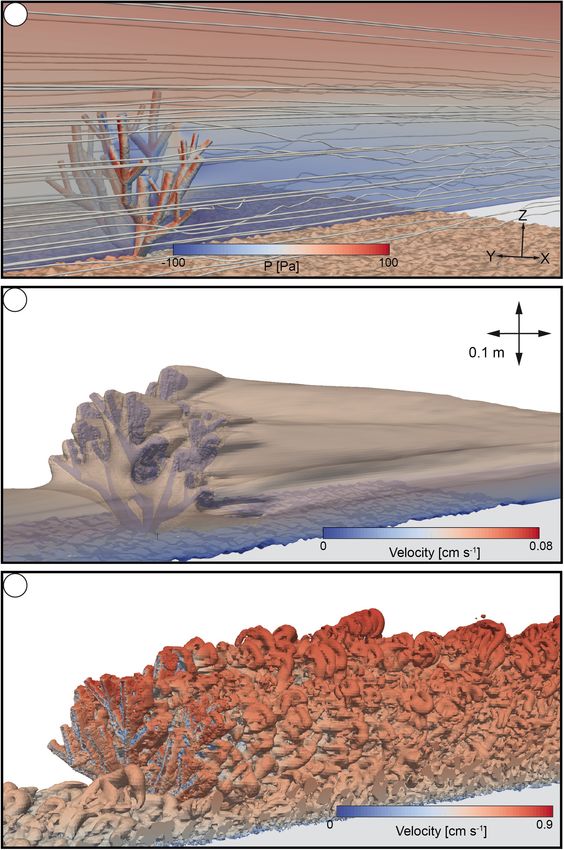
Bartzke et al.                                                                                              Hydrodynamics Around a Cold-Water Coral

i.e., do not carry symbionts, and favor colder water temperatures.          sediments stabilize the biogenic construction, and hence, favor
Among the cold-water corals the framework-forming                           mound aggradation (Huvenne et al., 2007; Thierens et al., 2013;
scleractinian species, also referred to as constructional,                  Titschack et al., 2015).
habitat-, reef-, or structure-forming corals, are of special                    The interplay between bottom current strength and the coral
importance (see Roberts et al., 2009). So far, most framework-              framework influences the amount of sediments baffled by the
forming scleractinian corals have been discovered in the North              corals. Hence, if suitable environmental conditions for corals
Atlantic, including the Gulf of Mexico, the Caribbean Sea,                  persist over sufficiently long periods of time, and coral growth
as well as the Mediterranean Sea (Wienberg and Titschack,                   is faster than sediment accumulation, substantial deposits of
2015). By forming reef-like structures, the framework-forming               coral mound material consisting of coral fragments and baffled
cold-water corals provide a refuge for a large number of                    sediments can form. Although this conceptual approach is widely
organisms and, consequently, the ecosystems formed by these                 accepted (e.g., Wienberg and Titschack, 2015), little is known
corals can be considered as impressive deep-sea biodiversity                about the prevailing sediment and fluid dynamical mechanisms
hotspots (e.g., Marshall, 1954; Henry and Roberts, 2015;                    in the direct vicinity of the corals.
Orejas and Jiménez, 2017).                                                      In this context, the question is to which extent the flow
    Over geological time scales, millennia and longer, such reef-           and the sediment dynamics are affected by the presence of
like structures can develop into coral mounds, three-dimensional            corals? To answer this question, the interplay of the prevailing
seafloor obstacles reaching heights from a few to >300 m                    hydrodynamics and sediment transport with corals should be
(Hebbeln et al., 2016). Consisting of fragments of the aragonitic           investigated on a high spatial and temporal scale. Many successful
coral skeleton and hemipelagic sediments, such coral mounds are             in situ surveys have been done over the last decades using
widely distributed along the continental margins of the Atlantic            various devices, such as landers or moorings (e.g., Guihen et al.,
Ocean (Hebbeln and Samankassou, 2015). They are found in                    2013; Mohn et al., 2014; Cyr et al., 2016). However, the data
shelf environments down to the upper and middle slopes and                  acquired with such investigations provides information about
are mostly arranged in large provinces that comprise hundreds               the general flow patterns near the reefs, but does not resolve
of individual mounds and cover extensive areas of several tens              the flow characteristics in the direct vicinity of the cold-water
of square kilometers (e.g., Paull et al., 2000; Wheeler et al., 2007;       coral colonies. In order to assess to which amount a cold-
Hebbeln et al., 2014, 2019; Vandorpe et al., 2014; Glogowski                water coral colony affects the flow, it is essential to measure
et al., 2015). Mound development is controlled by sustained coral           close to the seafloor next to a colony, particularly on the
growth and sediment supply (Hebbeln et al., 2016). The corals are           centimeter to meter scale.
controlled by a set of environmental boundary conditions, which                 Here, laboratory-based investigations may foster our process
include (i) physical and chemical properties of the surrounding             understanding. As highlighted by Mienis et al. (2019), literature
water masses (e.g., temperature, dissolved oxygen concentration,            broadly reports about flume studies with a background in
pH); (ii) food supply, which can be either phytodetritus or                 geoengineering where the focus was set on research, such as
zooplankton; and (iii) the local hydrodynamic regime providing              the flow alteration induced by underwater vegetation (e.g., Chen
food particles to the sessile suspension-feeding cold-water corals          et al., 2012) and their consequences for sedimentation with
(e.g., White et al., 2005; Mienis et al., 2007; Davies et al., 2009;        regard to the turbulent wake. From research about the nutrient
Davies and Guinotte, 2011; Flögel et al., 2014). The needed strong          supply of tropical corals, Chang et al. (2009) impressively showed
hydrodynamics are well-documented, by actual field surveys on               the prevailing hydrodynamics that occur within the branches
living cold-water coral settings. For example, at various sites in          of a tropical coral (Stylophora pistillata) by using a flume
the Atlantic current speeds in the range of several 10 s of cm s−1          experiment. Also, from research about a tropical coral canopy
have been measured in situ at and around coral mounds (e.g.,                (Porites compressa) Reidenbach et al. (2007) were able to resolve
Dorschel et al., 2007a; Mienis et al., 2007; Guihen et al., 2013;           hydrodynamic processes that occur near a coral canopy, such as
Hebbeln et al., 2014) with maximum speeds of ∼1 m s−1 (de                   the turbulences on the small scale by a flume experiment. With
Clippele et al., 2018; Lim et al., 2020). Laboratory experiments            regard to cold-water corals, Mienis et al. (2019) investigated in a
revealed that flow speed affects the feeding behavior of cold-water         flume experiment the prevailing hydrodynamics in the upstream
corals where Zooplankton is best captured at flow speeds below              and downstream reach of a cold-water coral patch, but did
2 cm s−1 , while phytodetritus is captured at higher flow speeds            not map flows within the interior, i.e., between the branches.
(Orejas et al., 2016).                                                      Consequently, little is known about the hydrodynamic conditions
    In addition to the proliferation of the corals, the development         within the direct vicinity of a cold water coral and specifically
toward coral mounds is further dependent on the capacity                    within or behind the branches and about the development of the
of the coral framework to entrap (baffle) bypassing sediment                turbulent wake, which are important factors affecting food supply
and thereby significantly increase sediment accumulation. For               and sediment transport.
example, from sediment cores collected from various cold-water                  Numerical models can help to overcome such limitations.
coral mounds it was shown that the amount of accumulated                    Even though, these models are simplifications of reality, they can
sediment, contributes >50% to the mound material (e.g.,                     provide remarkably useful approximations (aphorism attributed
Dorschel et al., 2007b; Titschack et al., 2009, 2015, 2016).                to George Box, 1978) and hence can be treated as a supplementary
Thus, the capability of the coral framework to baffle current-              tool for field or laboratory-based investigations in order to refine
transported sediments plays a crucial role as the entrapped                 the current understanding of the complex processes related to the

Frontiers in Marine Science | www.frontiersin.org                       2                                  September 2021 | Volume 8 | Article 663304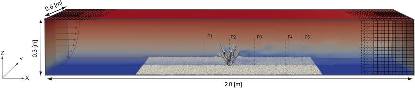
Bartzke et al.                                                                                            Hydrodynamics Around a Cold-Water Coral

effect of coral colonies on the flow and therefore sedimentation           In order to achieve these maximum flow speeds of 0.73 m s−1 ,
processes. Nonetheless, numerical simulation results are often             in the free stream, at the beginning of the test section toward the
challenged in the scientific community onto the accuracy of                downstream direction under steady uniform flow conditions, the
the simulation results. In order to overcome this challenge                slope of the flume was set to 4%.
and to demonstrate the capability of numerical simulations, we                 For the exact positioning of the measurement devices within
performed a set of hydraulic laboratory flume experiments to               the flume with respect to the desired measurement coordinates,
investigate the effects of a simplified cold-water coral colony            a traversing unit (Isel Automation KG) was installed above the
used as current obstacle on the prevailing hydrodynamics. The              test section and was connected to a control unit. An artificial
acquired data is used to validate a 3D numerical model. The                seabed with a surface roughness (D50 = 4 mm) that mimics the
cold-water coral structure used in the experiments mimics the              hardground that is typical for environments onto which cold-
shape of a cold-water coral colony that grew on a hard substrate           water corals may grow was installed at the bottom of the flume. It
at the bottom of the ocean. Notice, our attempt was not to                 is anticipated that this configuration resembles the hard substrate
replicate nature but to focus on the main flow features that               e.g., small coral fragments in sediment or a rocky seafloor, needed
are to be expected as the flow passes a simplified cold-water              for larvae settlement. Therefore, gravel in a grainsize ranging
coral colony. Moreover, we aimed on the quantification to which            between 2 and 8 mm was glued on a plate that is installed on
extent a colony is capable to alter the flow field and to reduce           the bottom wall over the entire test section. Furthermore, nubby
flow velocities.                                                           PVC mats were placed at the bottom of the flume ranging from
                                                                           the inlet to the test section.
                                                                               The cold-water coral model (Figure 1) was designed to mimic
MATERIALS AND METHODS                                                      a Lophelia pertusa colony, the most common framework-forming
                                                                           cold-water coral in the Atlantic Ocean, in a simplified manner.
Physical Experiment Description                                            Please notice that in our experimental setup we decided to
The hydraulic laboratory flume experiments were conducted                  use a simplified structure that served as a shape model to
in a unidirectional tilting flume at the Leichtweiß-Institute for          capture the main flow features within and in the rear of a
Hydraulic Engineering and Water Resources, TU Braunschweig                 cold water colony, which allows for a better comparison of the
(see Figure 1 for the experimental flume setup). The dimensions            results of the flume experiment and the numerical model. The
of the rectangular flume were X = 32.0 m in the downstream                 structure of the coral was generated using a computer aided
direction, Y = 0.6 m in the across stream direction and Z = 0.3 m          graphics design (CAD) program (AutoCAD) and was designed
for the mean water depth in the channel and it was filled with             with cylinders. The virtual structure was then printed using
freshwater with a temperature of 20◦ C, and a kinematic viscosity          an Ultimaker UM2 3D-printer. The filament used to print the
of 10–6 m2 s−1 . Notice that focus of this study is on the main            structure was a polylactide polyester (PLA), with a building
flow characteristics that occur in the case of a cold-water colony         strength of 103,0 MPa, produced by the company Dremel. The
in general. Therefore, slightly higher density values, as found in         final spatial dimensions of the simplified coral resulted in an
the ocean, would have a neglectable impact in the main flow                average height of 0.14 m and an average horizontal diameter of
characteristics. The discharge was controlled by a valve and               0.12 m. The cylindrical stem in the center of the simplified coral
measured by a Krohne Aquaflux inductive flow meter, which had              colony has a height of 0.07 m. In order to fix the structure at
a resolution of 0.01 l/s. Point gauges were installed to measure           the bottom of the flume, a screw thread was milled and glued
the water depth. The tilting slope, discharge and water depth              with a two-component glue into the bottom cylinder of the coral
were adapted in accordance to ensure stationary, uniform flow              model. In order to ensure a solid stance also at relatively high
conditions. The water depth was kept constant by a tailgate                flow speeds, the cold-water coral colony was positioned and
positioned at X = 25.5 m. In addition, to suppress the disturbance         fixated in the center of the test section. The exact location as
of the flow field by wave generation at the inlet flow straighteners       well as the orientation of the cold-water coral facing the flow
made of honeycomb perforated bricks were installed in the direct           were recorded as this information was needed for the three-
vicinity of the inlet. The test section for the experiments was            dimensional reconstruction of the exact same orientation and
located at 16.0 m downstream of the inlet and was 1.5 m in length.         position of the coral in the numerical experiment.
For the experiment a flow velocity of 0.73 m s−1 was selected,                 An Acoustic Doppler Velocimeter (ADV) Vectrino II with a
which is at the higher end of what is found at thriving cold-water         3D down looking probe was used to measure the time average of
coral sites in the ocean. Nevertheless, current speeds of several          the downstream velocity component (Ux) (Figures 1A,C). The
decimeters per second are a common feature in various regions              device was mounted on the automatic traverse, which enabled an
(e.g., Porcupine Seabight: Dorschel et al., 2007b; Rockall Bank:           accurate positioning of the probe. The velocity components could
Mienis et al., 2007; Campeche margin: Hebbeln et al., 2014; Cape           be measured with a sampling rate of 1–100 Hz. The diameter
Lookout: Mienis et al., 2014) with peak values of 1 m s−1 (Tisler          of the sampling volume was 6.5 mm and its height could be
Reef, de Clippele et al., 2018) to 1.1 m/s (Porcupine Bank; Lim            changed between 1 and 9 mm. In the present study, each point
et al., 2020). As the corals depend on the lateral food supply             was sampled with 100 Hz for 60 s. This ensured a representative
provided by bottom currents, we suppose that the above average             time averaged mean value of the flow velocity. The sampling (or
current speeds are the most favorable for the corals. For this             measuring) volume of the ADV is 5 cm below the probe, thus, it is
reason, we use a current speed of 0.73 m s−1 for this experiment.          not affected by the presence of the measuring device. The quality

Frontiers in Marine Science | www.frontiersin.org                      3                                 September 2021 | Volume 8 | Article 663304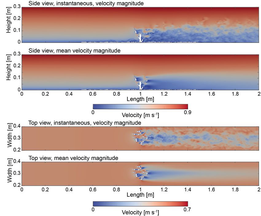
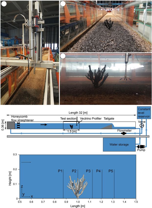
Bartzke et al.                                                                                                                   Hydrodynamics Around a Cold-Water Coral

  FIGURE 1 | Summary of the laboratory-based flume experiment. (A) Traversing unit mounted above the drained flume with installed Vectrino profiler. (B) View into
  the downstream direction of the drained flume with the mounted cold-water coral model and roughness elements. (C) Sideview of the experiment showing the
  cold-water coral model as well as the Vectrino profiler. (D) Schematic of the setup of the flume experiment. (E) Positions of the reference profiles in the test section.

Frontiers in Marine Science | www.frontiersin.org                                     4                                         September 2021 | Volume 8 | Article 663304
Bartzke et al.                                                                                            Hydrodynamics Around a Cold-Water Coral

of the measurements was ensured by two parameters: signal to              and are computational cost efficient (Gritskevich et al., 2012).
noise ratio above 25%, and correlation parameter. The correlation         This technique has been broadly used in aerospace engineering
parameter serves as an indicator of the relative consistency of           (Viswanathan et al., 2007; Keylock et al., 2011; Shur et al., 2011),
the behavior of the scatterers in the sampling volume during              and geophysics (Alvarez et al., 2017). A DES simulation is a
the sampling period, which was at least above 85%. In total five          hybrid technique for turbulence modeling combining RANS
profiles arranged in a line were acquired using the Vectrino II for       (Reynolds-averaged Navier–Stokes equations) near the bed and
the validation of the numerical simulation results.                       the coral and a LES (Large Eddy Simulation) for the simulation of
    All profiles ranged from Z = 0.0 m to Z = 0.2 m in height,            the flow interior, aiming to alleviate the costly near-wall meshing
except Profile 2, which ranges from Z = 0.07 m to Z = 0.2 m               requirements imposed by the LES. According to Gritskevich et al.
due to its position above the coral colony. The profiles were             (2012) the original intent of DES was to be run in RANS mode
laterally spaced 0.1 m apart with Profile 1 being located at              for attached boundary layers and to switch to LES mode in large
X = 0.9 m downstream from the inlet, Profile 2 at X = 1.0 m,              separated (detached) flow regions. Regions near solid boundaries
Profile 3 at X = 1.1 m, Profile 4 at X = 1.2 m, and Profile 5 at          and where the turbulent length scale is less than the maximum
X = 1.3 m (Figure 2). The respective Y coordinate was located             grid dimension are assigned the RANS mode of the solution. As
at the center of the flume at Y = 0.3 m. For each profile 51              the turbulent length scale exceeds the grid dimension, the regions
points were acquired, whereby the vertical distance between the           are solved using the LES mode. Therefore, the grid resolution is
measurement points was 1z = 0.4 cm. Due to the structure of the           not as demanding as in the case of a pure LES, and is thereby
coral, Profile 2 which is located above the major coral trunk only        considerably cutting down the cost of the computation. This
had 34 measurement points. Measurements close to the water                strategy allowed for the computation of the model results on a
surface were not obtained to exclude bias from potential surface          standard workstation on 12 cores.
water movements.                                                             The LES equations are derived by applying a spatial filtering
    In order to reconstruct the surface roughness for the                 operation. These equations are shown below in terms of the LES
numerical model the gravel bed was scanned over the entire                decomposition:
length of the test section after the flume was drained. This was                                              δui
                                                                                                 Continuity        = 0                     (1)
done by defining a raster of measurement points over the test                                                 δxi
section in a 1x = 1.6 mm and 1y = 2 mm spacing. The resulting
point cloud was then filtered, interpolated, and meshed into a STL
                                                                                          δui   δ(ui uj )        1 δp     δ              δui
file (STereoLithography file). The point cloud was interpolated            Momentum           +            = −         +     ((ν0 + ν0t ) )
using the Matlab function gridfit. By the combination of the                               δt       δxj          ρ δxi   δxi             δxi
coral model and the surface roughness files a single STL file was                                                                            (2)
generated that was imported into a numerical Computational-               where u and p are the velocity and pressure components,
Fluid-Dynamics (CFD) environment for further treatment.                   % is the density, ν is the kinematic viscosity, and νt is the
                                                                          turbulent eddy viscosity. The term on the right hand side of the
                                                                          momentum equation containing the kinematic viscosity and the
Numerical Model Description
                                                                          eddy viscosity (ν0 + ν0t ) represents the unresolved subgrid (SGS)
To investigate the flow within the test section of the hydraulic
                                                                          stress tensor, and is modeled using the Spalart-Allmaras (S-A)
laboratory flume channel and in the direct vicinity, as well as,
                                                                          turbulence closure. The S-A model has the advantage of being
in the rear of the cold-water colony and hence that is used as a
                                                                          a non-zonal technique, implying that one single momentum Eq.
shape model to capture the main flow features, a numerical CFD
                                                                          (2) can be used with no a priori declaration of the RANS vs.
model was used based on the open source toolbox OpenFOAM
                                                                          LES zones. The length scale of the S-A model is equal to the
(Open Field Operation and Manipulation). This C++ based
                                                                          minimum of the distance to the bed and the coral, and the
software package provides a wide range of solvers that are readily
                                                                          length scale proportional to the local grid spacing(CDES 1G ).
compiled, but also may be personalized by the user for individual
                                                                          Thus, d̃ = min d, CDES 1G provides a way to make a transition

purposes (Schmeeckle, 2014; Bartzke et al., 2018). In order to
resolve the flow equations OpenFOAM uses the Finite Volume                between RANS and LES by retaining RANS within the boundary
Method (FVM). The study domain is discretized into a grid                 layer when d̃ < d and applying LES to the zone away from the
of three-dimensional hexagonal elements, over which volume                bed or the coral when d̃ ≥ CDES 1G . In more detail a Spalart-
integral formulations of conservation equations are applied.              Allmaras IDDES (Improved Delayed Detached Eddy Simulation)
Variables, such as the pressure scalar, and velocity vector are           was used. The IDDES is based on original formulation Spalart-
stored at the center of each control volume i.e., cell of the mesh.       Allmaras DES model (Spalart et al., 2006) but uses a modified
In the present study OpenFOAM version 1706 was used.1                     improved formulation of the length scale to solve the unresolved
   For the simulation of turbulence in the numerical model, a             subgrid (SGS) stress tensor (Gritskevich et al., 2012). The
Detached Eddy Simulation model (DES) was used. The choice of              performance of this model has been extensively tested and
this model type was inspired by industrial CFD simulations that           verified on a large set of test cases (Gritskevich et al., 2012). In
rely on Scale-Resolving Simulation (SRS) models, which resolve            the present study, the standard OpenFOAM solver pisoFoam
the turbulence spectrum in at least a part of the flow domain             was used for velocity pressure coupling for time dependent
                                                                          flows. The PISO (Pressure-Implicit with Splitting of Operators)
1
    www.openfoam.com                                                      algorithm (Issa, 1986) is a pressure correction scheme used to

Frontiers in Marine Science | www.frontiersin.org                     5                                   September 2021 | Volume 8 | Article 663304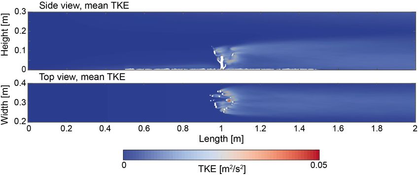
Bartzke et al.                                                                                                                      Hydrodynamics Around a Cold-Water Coral

  FIGURE 2 | Setup of the numerical model domain showing the position of the roughness elements and the cold-water coral model as well as the exact locations of
  the processed fluid profiles. The profile on the left indicates the flow distribution at the inlet. The mesh at the right side indicates the used resolution levels used in the
  numerical model.

calculate the pressure distribution correction to derive the local                          entering the domain on the left side of the domain (upstream)
velocity field toward a result that satisfies both momentum and                             and leaving it on the right (downstream). Notice that the mapped
continuity (Ferziger and Perić, 2002). Please note, to interpret the                       profile of the flume experiment was time averaged and did
results from this incompressible solver, the kinematic pressure                             not exhibit any fluctuations over the entire simulation time,
was multiplied by the density (%) value (OpenFoam User Guide).                              but ensured a constant flow into the model domain. Physical
                                                                                            properties in the numerical model were chosen to mimic an
                                                                                            incompressible fluid. The kinematic viscosity ν was set to 1e-
Numerical Model Setup                                                                       6 m2 /s implying a density (ρ) of 1,000 kg/m3 . In order to
The numerical model domain was setup to replicate the                                       ensure the comparability of the model results with those of the
test section of the laboratory-based flume experiment with                                  flume experiment the same physical parameters were chosen,
dimensions of 2.0 × 0.6 × 0.3 m (Figure 2). The coral was                                   which represent the physical properties of freshwater. Each
positioned in the center of the domain at X = 1.0 m and Y = 0.3 m.                          calculation run simulated a total time of 30 s with a time step of
The coral in the numerical simulation as well as in the flume                               0.0025 s. The simulation was numerically stable showing Courant
experiment had the same orientation. The computational mesh of                              numbers smaller than 0.2. The numerical simulation was run in
the domain was constructed from a background mesh (mesh level                               parallel on a single workstation (Intel Xeon CPU E5-2650 v4 @
0; 400 × 60 × 30 cells). This background mesh was refined using                             2.20 GHz) on 12 processors, whereby the entire computation time
a refinement box ranging from X = 0.0 to 2.0 m, from Y = 0.2                                lasted for 16 days.
to 0.4 m, and from Z = 0.0 to 0.3 m. The cell dimensions in
the refinement box were 50 percent smaller as compared to the
background mesh (mesh level 1, 800 × 80 × 60 cells). In order to                            Data Analysis
resolve the fluid dynamical processes in the vicinity of the coral                          Please note that only the data after 20.0 s of simulation time was
colony as well as near the pebble bottom in highest resolution                              considered for further evaluation to ensure that the flow traveled
a surface wise refinement was applied. The surface refinement                               once through the entire domain but also to avoid backward
was defined to cover all cells located at a maximum of 0.05 m                               flow at the outlet. All data processing was either performed
apart from the coral colony or the bottom (mesh level 1–3). This                            with Matlab or with the inbuilt utility paraFoam, a customized
procedure resulted in 12,746,939 cells in total. The meshing of the                         version of Kiteware’s ParaView that comes with the OpenFOAM
coral colony and the bottom was performed with the OpenFOAM                                 software environment.
inbuild utility snappyHexMesh that allows to mesh structures                                   Flow velocity profiles from the numerical model were taken
into the background mesh.                                                                   at the same positions as in the experimental flume with the
    An inlet boundary condition was imposed at the left sidewall                            goal of comparing the two approaches. The velocity profiles
and an inlet/outlet boundary condition was assigned at the                                  obtained by the flume experiment were acquired as a time
right sidewall. No-slip boundary conditions were assigned to the                            average. In order to provide additional information about the
front, bottom, and back walls of the domain. The same applies                               instantaneous flow behavior, we also plotted the corresponding
for the gravel as well as for the coral structure located in the                            instantaneous velocity components. Each profile consisted of 200
center of the domain. The boundary condition chosen at the                                  datapoints in the vertical direction with increments of 1.0 mm.
top wall was a slip boundary condition, so no flux could pass                               The time average profiles were processed for comparison with
through this wall. In order to force the flow in a comparable                               the profiles obtained by the flume experiment by averaging the
manner to the flume experiment, a velocity profile from the                                 instantaneous flow speed values over time. The time average
beginning of the test section of the flume experiment was mapped                            of the instantaneous profiles was computed over 10 s with
and applied as inlet boundary condition. The maximum flow                                   increments of 0.1 s. In order to highlight the effect of flow speed
speed was U = 0.73 m s−1 . Notice that this velocity value was                              changes by the presence of the cold-water coral, the downstream
chosen to reflect the relative strong current speeds reported by                            velocity component (Ux) was processed. The same procedure
Lim et al. (2020). As a result, the flow became unidirectional by                           was applied for the transversal (Uy) and vertical (Uz) velocity

Frontiers in Marine Science | www.frontiersin.org                                       6                                          September 2021 | Volume 8 | Article 663304
Bartzke et al. Hydrodynamics Around a Cold-Water Coral
components. In order to aid visualization a set of slices was cut This led to a computed drag coefficient CD of 0.71 by taking
through the domain facing in the Y normal and the Z normal of an averaged velocity value (Ux) of 0.55 m s−1 , a surface area
the model domain. The slices indicate the instantaneous as well of 0.041 m2 , a density of 1,000 kg/m3 , and a Reynolds number
as the mean flow conditions without the velocity fluctuations. of 77000, into account. Notice that also the Drag coefficient
On the contrary, the velocity fluctuations are highlighted by can be post-processed within paraview (Kiteware) or with the
the instantaneous velocities. The same approach was done to postprocessing toolbox of OpenFoam.
highlight the distribution of the pressure field as well as for the
turbulent kinetic energy (TKE) values.
All profiles were extracted from a time averaged Y normal slice
at Y = 0.3 m and Z normal slice at Z = 0.05 m. The downstream RESULTS
positions of the solid lines represent profiles that were extracted
in the rear of the coral. In total 37 individual profiles were Flow Velocity Profiles Obtained With the
extracted from the numerical model between 1.1 and 2.0 m. Laboratory Flume
To compare the velocity data of the numerical model to the In total five-time averaged velocity profiles indicating the vertical
data of the flume experiment the coefficient of determination distribution of the downstream velocity component Ux were
R2 = 1 − SSreg /SStot was computed. Therefore, the sum of processed from the flume experiment (Figure 4). In order to
(yi − fi )2 of capture changes in the horizontal flow component with respect
P
squares of the regression (SSreg ), where SSreg =
the time averaged velocity values (Ux) from the model (yi ) and to the presence of the coral all profiles were located in the center
the corresponding experimental of the test section traversing in a line from the upstream to
P data (f2i ) and the sum of squares
total (SStot ), where SStot = (yi − y) of the model (yi ) and the the downstream reach of the test section. Profile 1 served as a
mean values of the model (y) were calculated. reference profile to measure the flow speed values upstream of the
In order to visualize typical features that can be processed coral. From the bottom of the bed to a height of 0.04 m the shape
from a CFD model, such as the streamlines and the drag of the Profile 1 indicates a curved pattern of the flow velocity
distribution (Figure 3A), the flow velocity contour (Figure 3B), value distribution due to the roughness of the hardground at the
and the Q-criterion (Figure 3C) in three-dimensions the software bed. Velocity values in that area range from 0.0 to 0.4 m s−1 .
paraview (Kiteware) was used. Toward the top the velocity values of profile 1 increase to
Please note that the results shown in Figure 3 were all 0.72 m s−1 . In the case of Profile 2 that was extracted right above
derived from the same timeframe at 25.0 s. The streamlines the central stem of the coral colony a clear deflection with respect
are shown as an example case in three dimensions. The same to the reference profile can be observed. The maximal change
applies for the isosurfaces to highlight the flow shading zone of the velocity values is indicated between the top of the coral
using a velocity contour of 0.08 m s−1 . In addition, the stem to 0.12 m. The velocity values here increased from 0.0 to
Q-criterion as well as the drag forces were processed with 0.6 m s−1 . Above 0.12 m toward 0.2 m the pattern of profile
the inbuilt filters of paraFoam (Kiteware). The Q-criterion 2 seems to reattach the shape of the reference profile 1. This is
[Q = 0.5 (2 −S2 )] is a vortex identification method and was indicated by a linear increase of the flow speeds values from 0.12
used to visualize the development of turbulences as isosurfaces. to 0.72 m s−1 toward the top. Profile 3 is characterized by an
Here, S and Omega are the symmetric and antisymmetric oscillating pattern of velocity values, ranging from the bottom
components of the velocity gradient tensor, where S is the at 0.0 m toward 0.14 m. In this region the flow velocity values
rate of strain tensor and Omega the vorticity tensor. By increase from 0.0 m s−1 at the bottom to 0.5 m s−1 at 0.14 m.
definition, a vortex is located where Q > 0. Notice that the Similar to profile 2 but with an offset of 0.02 m, a trend of linearly
Q-criterium can be post-processed within paraview (Kiteware) increasing velocity values can be observed. This distribution
or with the postprocessing toolbox that comes with the appears also to match with the shape of the reference profile. The
OpenFoam environment. corresponding velocity values ranged between 0.5 m s−1 at 0.12 m
Based on the pressure field values, the drag force was to 0.72 m s−1 at the top. In comparison to the two prior profiles
computed to show the impact of the hydrodynamic forces the pattern of Profile 4 appeared smoother in shape. Similar to
acting on the coral. Therefore, the surface planes of the coral profile 3, between 0.0 and 0.06 m a velocity increase to 0.18 m s−1
were extracted. The corresponding pressure values were then can be observed. Up to a height of 0.14 m the velocity increase is
multiplied by the surface normal values with respect to their more pronounced as compared to the section below, where the
direction. For example, the surface normals facing in the velocity values increase toward 0.5 m s−1 . Above, in the region
downstream direction were multiplied with the pressure values. from 0.14 m to the top, a similar distribution compared to the
This resulted in the drag force vectors acting on the individual reference profile can be observed. Here a maximal velocity value
branches of the coral. Subsequently, all values were integrated of 0.72 m s−1 was measured similar to the other profiles. Profile 5,
to gain the desired drag force. Notice that this value was the indicates a smoother pattern as compared to profile 4. However,
result of averaging over 10.0 s of model time. After computing in the lower part of profile 5 between 0.0 and 0.09 m, in average
the drag force, the drag coefficient (CD) can be computed as 0.01 m s−1 higher velocity values were measured as compared
CD = Drag/(V 2 A/2). Drag refers to the dragforce, refers to the to profile 4. Similar to the prior cases the upperpart of profile 5,
fluid density, V refers to the far field flow velocity, and A refers to between 0.15 and 0.2 m in height, the velocity values appeared to
the surface area. reattach, showing a similar pattern as compared to profile 1.
Frontiers in Marine Science | www.frontiersin.org 7 September 2021 | Volume 8 | Article 663304Bartzke et al. Hydrodynamics Around a Cold-Water Coral FIGURE 3 | (A) Rendered 3D image of the streamlines and pressure drag values affecting the cold-water coral model as well as roughness elements at the bottom of the domain. The transparent 2D slice in the center of the domain indicates the flow field. (B) Rendered isosurface, indicating flow velocity values of 0.08 m s– 1 . (C) Rendered isosurface indicating the Q-criterion. Frontiers in Marine Science | www.frontiersin.org 8 September 2021 | Volume 8 | Article 663304
Bartzke et al.                                                                                                           Hydrodynamics Around a Cold-Water Coral

  FIGURE 4 | (A–E) Fluid profiles processed from the laboratory-based flume experiment as well as from the numerical model.

Flow Velocity Profiles Obtained With the                                             (Figures 5A,C). Slight fluctuations within the flow field can
Numerical Model                                                                      be observed in the case of the instantaneous flow field near
                                                                                     the bottom indicating the deflection of the flow velocity values
For the validation of the numerical model the downstream facing
                                                                                     near the roughness elements (Figures 5A,C). In general, velocity
flow velocity values were plotted against those obtained by the
                                                                                     magnitude changes were largest in the regions where the branches
flume experiment. Moreover, for a better representation of the
                                                                                     touched the freestream, exhibiting values of 0.7 m s−1 , whereas
model results both the instantaneous velocity values as well
                                                                                     the lowest values were derived in within the coral and ranged
as the time averaged values were plotted (Figures 4A–E). For
                                                                                     between 0.0 to 0.05 m s−1 (Figures 5A,C). Both minimum and
all measuring points, the time averaged profiles of both the
                                                                                     maximum values are concentrated in patches located in the direct
numerical and the flume channel experiment are in excellent
                                                                                     vicinity of the coral branches forming alternating regions of low
agreement. Particularly the shape of the velocity distributions
                                                                                     and high velocity fields. Detailed observation of the slices both
(Ux) of profile 1 (R2 = 0.99), profile 4 (R2 = 0.98), profile 3
                                                                                     in the vertical and horizontal directions indicates that the flow
(R2 = 0.98), and profile 5 (R2 = 0.99) indicated a nearly perfect
                                                                                     separates as it encounters the branches of the corals. In particular,
match. A slight underestimation of the flow speeds with respect
                                                                                     the instantaneous velocity fields (Figures 5A,C) showed that the
to the time averaged velocity component is present in the case
                                                                                     flow values are generally higher in front of the branches and
of profile 2 (R2 = 0.77). Nonetheless, the goodness of the results
                                                                                     lower in their rear, where the fields are disturbed. The flow field
is further supported by the distribution of the instantaneous
                                                                                     above the coral appeared unaltered (Figures 5A,B). In contrast
velocity profiles, which clearly indicate that the overall velocity
                                                                                     to the homogeneous distribution of the flow velocity field in the
fluctuations match the pattern of the profiles measured by the
                                                                                     upstream reach, a pattern of fluctuating velocity values becomes
flume experiment.
                                                                                     visible downstream from the coral toward the end of the domain.
                                                                                     The fluctuations within the flow field can be directly observed
Flow Field Derived With the Numerical                                                in the case of the instantaneous flow field in the direct rear of
Model                                                                                the coral, where a reduction of the flow velocity values can be
Two slices were cut through the domain facing in the Y                               observed. For example, at a height of 0.05 m, from the upstream
normal and Z normal direction in order to highlight velocity                         reach at (X = 0.9 m) toward the direct rear of the coral colony
field patterns (Figure 5). In addition to the instantaneous                          (X = 1.1 m) the decrease of the flow speeds was 0.3 m s−1 .
(Figures 5A,C), also the time averaged values are shown as mean                      This reduction is indicated in both the side and top views in
velocity magnitude (Figures 5B,D). The flow velocities observed                      Figure 5. The height of this zone is successively thickening
between the inlet of the domain and the coral exhibit an almost                      from 0.12 m at 1.1 m toward 0.16 m at 2.0 m (Figures 5A,B).
homogenous flow field with a logarithmic gradient from the                           The shape of this zone appears to form a curved region that is
bottom to the top indicating a mean velocity value of 0.58 m s−1                     characterized by patches of fluctuating velocity values that are

Frontiers in Marine Science | www.frontiersin.org                                9                                      September 2021 | Volume 8 | Article 663304
Bartzke et al. Hydrodynamics Around a Cold-Water Coral
FIGURE 5 | (A) Side view (Y = 0.15 m) indicating the instantaneous flow field at 25.0 s. (B) Side view (Y = 0.15 m) of the time averaged flow field. (C) Top view
(Z = 0.05 m) indicating the instantaneous flow field at 25.0 s. (D) Top view (Z = 0.05 m) of the time averaged flow field.
lower as compared to the upstream reach, and is defined here as of the coral (white colored profiles in Figure 6A) differ from
the low velocity zone. the pattern of the reference profile and are characterized by an
undulated distribution of the flow velocity values. For example,
the profile that was extracted directly from the rear of the coral
Downstream Evolution of the Flow appeared disturbed in shape. Toward the top of the profile, in the
Velocity Profiles Obtained With the range between 0.12 to 0.18 m the pattern of the profile appears to
Numerical Model reattach to the original shape of the reference profile. With further
In order to aid visualization of the flow velocity distribution, the distance into the downstream direction the shapes of the profiles
time averaged flow speeds facing into downstream direction that appeared smoother and tend to transform into a linear pattern
were derived from the numerical model are shown in Figure 6. with height. In addition, a shift of the velocity value distribution
All flow profiles are characterized by relatively low flow velocity with respect to the distance further in the downstream direction
values close to the bottom of the domain and increase with becomes evident. For example, all values that were extracted in
respect to height (Figure 6A). In the case of the reference profile the range between 0.0 and 0.12 m close to the rear of the coral are
indicating the undisturbed flow speed values upstream of the characterized by relatively low flow speeds. i.e., low velocity zone.
coral (dashed lines in Figure 6) the velocity values increase from However, those profiles that were extracted further downstream
0.0 m s−1 at the bottom toward 0.4 m s−1 at 0.06 m. In this indicate a trend of successively increasing values (black colored
region the profile is characterized by a parabolic shape. Further profiles in Figure 6A). For example, the profile that was extracted
toward the top of the profile the velocity values increase in a in the far region of the domain is characterized by a straight
linear pattern to 0.7 m s−1 . The profiles extracted in the vicinity pattern showing a velocity increase ranging between 0.3 m s−1
Frontiers in Marine Science | www.frontiersin.org 10 September 2021 | Volume 8 | Article 663304Bartzke et al. Hydrodynamics Around a Cold-Water Coral
at 0.01 m and 0.45 m s−1 at 0.12 m. The velocity increase in the pattern of the pressure values changed, which is indicated
this region averaged 0.22 m s−1 with respect to the distance by negative values in the range of –90 Pa. The pressure values
into the downstream direction. An opposing trend of decreasing within the center region as well as in the direct rear of the coral
velocity values that is indicated by the position of the profiles with appeared concentrated into patches in the rear of the respective
respect to their distance into the downstream direction, can be branches. Similar to the pattern indicated by velocity magnitudes
observed in the region above 0.12 m. The flow profiles that were (Figure 6), the instantaneous values in the range from the rear
extracted in the vicinity of the coral initially appear to match with of the coral toward the end of the domain indicated a thickening
the velocity distribution of the reference profile ranging between pattern of fluctuating pressure values ranging between –50 and
0.55 m s−1 at 0.12 m toward 0.7 m s−1 at 0.2 m. However, with 50 Pa. The same trend can be observed with respect to the top
increasing distance into the downstream direction the flow speed view (Figure 7B) by which a conical narrowing out toward the
values successively decrease, whereas a transformation from an end of the domain of the pressure fluctuations can be observed.
initially parabolic shape into a linear shape becomes obvious. The The TKE values were derived as an additional field to
velocity decrease in this region averaged at 0.2 m s−1 with respect characterize the mean kinetic energy per unit mass that is
to distance of the profiles facing into the downstream direction. associated with eddies that form in a turbulent flow (Figure 8).
For the profiles extracted over the width of the model The side view indicates TKE values in the range of zero within
(Figure 6B) a similar trend of increasing flow speed values into the region from the inlet toward the front of the coral. Increased
the downstream direction can be observed. The velocity ranges values can be observed in the vicinity of the rough bottom.
of the reference profile indicated a uniform velocity distribution In the center region of the coral from 0.9 to 1.1 m, the TKE
over the entire width of the domain of 0.48 m s−1 at 0.08 m. values increased to a maximum of 0.05 m2 /s2 , and averaged at
All flow velocity profiles in the downstream region of the coral 0.02 m2 /s2 . This indicates that the highest amount of TKE is
are characterized by a parabolic distribution of the flow velocity distributed in the direct vicinity of the coral branches. From the
values. Highest values were measured further away from the coral rear of the coral toward the end of the domain the TKE values
toward the side walls of the domain at 0.2 and 0.4 m. Lowest remained in the similar range of 0.02 m2 /s2 but successively
values were obtained from the center of the domain in the range deceased to 0.03 m2 /s2 toward the downstream end of the
between 0.28 and 0.32 m (Figure 6B). For example, the minimal domain. The width of the TKE field remained relatively constant
values of the profile that was located in the direct vicinity of from the rear of the coral colony toward the end of the domain
the coral (white colored profiles in Figure 6B) were 0.13 m s−1 and ranged between 0.22 and 0.38 m.
and increased to a flow speed of 0.55 m s−1 toward the sides,
indicating a decrease of the flow speeds by 0.42 m s−1 over the
entire model width. However, with increasing distance further Streamlines, Pressure Drag, Velocity
into the downstream direction, the pattern of the velocity values Deflection, and Q-Criterion
appear to smooth out, which is indicated by an almost perfectly In order to demonstrate additional capabilities of the numerical
shaped parabolic distribution of the velocity values with respect model, and hence, to improve the understanding of the flow
to width (black colored profiles in Figure 6B). For example, in with respect to the presence of a cold-water coral colony a set
the case of the profile located at 1.9 m, the velocities were lowest of analysis tools that are common in the field of Computational-
within the center of the domain, which is indicated by a velocity Fluid-Dynamics were summarized for an overview: (i) 3D-
value of 0.4 m s−1 , whereas the flow speeds at the sides of the visualization of streamlines and the pressure drag distribution
domain appeared to reattach to the shape of the reference profile affecting the coral (Figure 3A); (ii) the flow velocity contour
to 0.5 m s−1 . Comparing the differences of the flow velocity (Figure 3B), and (iii) the Q-criterion (Figure 3C), with all data
values of the profiles close to the coral to those from the end are derived from the same timeframe at 25.0 s. This graph aids the
of the domain taken in the range of the centerline, a difference visual representation of the hydrodynamics and ultimately will
of 0.32 m s−1 over a distance of 1.0 m into the downstream implicate a basis to derive information on the impact of changing
direction was derived. hydrodynamics on sediment dynamics in a future study.
All streamlines located upstream of the coral colony were
oriented in a parallel pattern indicating a homogeneous flow
Pressure Field and Turbulent Kinetic (Figure 3A). A transition toward a chaotic arrangement of the
Energy Field streamlines becomes evident in the rear of the coral colony and is
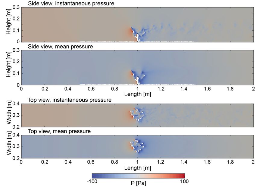
The pressure fields of the instantaneous as well as the time also evident further into the downstream direction ranging over a
averaged flow field are shown in a side and top view that height of Z = 0.0 m to Z = 0.12 m. The streamlines above the coral
was sliced through the model domain (Figure 7). The pressure in the range of 0.12 and 0.3 m appear to resume parallel pattern.
distribution between the inlet of the domain and the coral colony The pressure values affecting the coral colony were highest in the
exhibit an almost homogenous pressure field in the water column regions of the branches of the coral that faced the flow. Negative
as well as in the regions close to the bottom. The pattern of the pressure values were observed in the regions where the branches
pressure field in the vicinity of the coral colony appeared highly opposed the flow direction. The respective drag forces revealed a
diverse. Highest pressure values were observed in the range value of 0.971 N. The deflection of the flow field with respect to
where the branches faced the flow, which is indicated by values the coral colony is shown in Figure 3B. The three-dimensional
peaking at 80 Pa. In the region within the center of the coral, representation shows an isosurface that was processed to indicate
Frontiers in Marine Science | www.frontiersin.org 11 September 2021 | Volume 8 | Article 663304Bartzke et al. Hydrodynamics Around a Cold-Water Coral FIGURE 6 | (A) Profiles indicating the downstream velocity component with respect to model height (Z = 0.05 m). (B) Profiles indicating the downstream velocity component with respect to model width (Y = 0.15 m). The 37 individual profiles were extracted from the model between 1.1 and 2.0 m. The white color refers to profiles that were extracted close to the coral, whereas the black colors references to profiles that were located further downstream of the coral. The dashed line indicates the profile that was extracted before the coral. For comparison, the dashed lines refer to an undisturbed reference profile measured at 0.9 m in the upstream reach of the coral. FIGURE 7 | (A) Side view (Y = 0.15 m) indicating the instantaneous pressure field at 25.0 s. (B) Side view (Y = 0.15 m) of the time averaged pressure field. (C) Top view (Z = 0.05 m) indicating the instantaneous pressure field at 25.0 s. (D) Top view (Z = 0.05 m) of the time averaged pressure field. a three-dimensional surface that represents the distribution of velocity zone that ranges from the rear toward the end of the all velocity values lower than 0.08 m s−1 as an example case. domain. Moreover, the isosurface indicates that this hull was The hull appears as a conical shaped shadow indicating the low lower in height in the upstream direction and appeared lower in Frontiers in Marine Science | www.frontiersin.org 12 September 2021 | Volume 8 | Article 663304
Bartzke et al.                                                                                                                 Hydrodynamics Around a Cold-Water Coral

  FIGURE 8 | (A) Side view (Y = 0.15 m) indicating the turbulent kinetic energy (TKE) field as a time average. (B) Top view (Z = 0.05 m) indicating the turbulent kinetic
  energy field as a time average.

height in the rear of the coral as well. This highlights the effect                      the profiles of the numerical model was 10 Hz. Nonetheless
of a reduction of the flow velocity values with respect to height.                       a higher sampling frequency would have exceeded our storage
For example, the height of the isosurface was at 0.05 m in the                           capacities. Nonetheless, the pattern of the instantaneous and
upstream region, and at 0.14 m in height in the downstream                               time averaged profiles reflects an excellent agreement with the
region. This indicates a deflection of the initial flow field by 9 cm                    velocities obtained by the flume experiment, which greatly
in terms of height and corresponds to a factor of 2.8 with respect                       demonstrates the fidelity of the numerical model results.
to the measured height difference. Furthermore, as an indicator                              With respect to the evolution of the flow field, the
for turbulent flow structures, the Q-criterion was processed as                          instantaneous velocity profiles indicated velocity fluctuations
an isosurface (Figure 3C). Coherent structures can be observed                           at the bottom and in the direct vicinity as well as in the
near the bottom of the upstream region before the flow reached                           rear of the cold-water coral colony. These fluctuations can be
the coral. In the area where the branches of the coral faced the                         related to turbulences generated due to the rough bottom as
flow for the first-time, coherent structures also appeared to form.                      well as due to the presence of the coral opposing the flow
A similar trend can be observed within the center of the coral.                          as an obstacle. Main flow features observed in the range of
In the region ranging from the rear of the coral toward the end                          the coral include the presence of flow separation zones along
of the domain the pattern of the isosurfaces is characterized by a                       the individual branches of the cold-water coral mixing up into
large number of alternating vortexes that appear to migrate in a                         turbulent zones. This is indicated by alternating patches of flow
staggered pattern toward the end of the domain.                                          speed values, pressure values, as well as, TKE values (Figure 8).
                                                                                         Downstream from the coral the vortices form into a lee-wake
                                                                                         vortex shed. The shape of the vortex shed behind the coral
DISCUSSION                                                                               corresponds well to the appearance of the low velocity zones as
                                                                                         indicated by the flow speed measurements (Figures 4–6). It is
Flume Channel and the Numerical                                                          also comparable to the distribution of the enhanced TKE values
Experiment Data                                                                          (Figure 8) extending from the rear of the coral downstream.
The velocity profiles obtained from the flume and the numerical                          This indicates that the presence of the coral causes a reduction
experiment show excellent agreement, and hence demonstrate                               in the flow speeds, but also initializes turbulences. The pattern
the predictive capabilities of the DES model with respect to                             of the flow field changes as the flow encounters the individual
the chosen parameters. The instantaneous profiles as well as                             coral branches and separates in the regions where the pressure
the time averaged profiles obtained with the numerical model                             is highest (Figures 5, 6). Regions of low pressure appear in
are in agreement with the flume experiments as shown by the                              the rear of the branches, resulting from the interaction between
coefficient of determination values. Nonetheless, one might argue                        the unidirectional flow and the coral branches. The interplay
that the model might slightly tend to underestimate the flow                             of developing flow separation zones and producing a pressure
conditions of the flume experiment in the cases of profiles 2                            gradient from the front toward the rear of the branches favors
and 3 (Figure 4) by a maximum of 0.08 m s−1 in the bottom                                the generation of downstream wakes. These can be compared
region. However, this offset can be related to the sampling rate                         to flows around cylinders as shown, for example, by Graf and
and hence is dependent on the amount of instantaneous profiles                           Istiarto (2002) or Chen et al. (2012). According to Roulund et al.
available to compute the time average. The sampling rate of the                          (2005) these vortices are caused by the rotation in the boundary
Vectrino profiler was set to 100 Hz to produce the time averaged                         layer over the surface of the pile, or in this case the branches of
flow velocity profiles, whereas the sampling rate to produce                             the coral. The shear layers emanating from the side edges of the

Frontiers in Marine Science | www.frontiersin.org                                   13                                        September 2021 | Volume 8 | Article 663304
Bartzke et al. Hydrodynamics Around a Cold-Water Coral
pile roll up to form these vortices in the lee wake of the pile. This on the lee side of the coral (cf. Orejas et al., 2016), especially
flow pattern is also evident in the rear of the coral branches and keeping in mind coral colony sizes of up to 1 m arranged in
called vortex shedding or a turbulent wake. Further downstream larger clusters of colonies (Fanelli et al., 2017; Vad et al., 2017). In
the vortices initialized by the branches contain eddying motions. addition, as indicated by the drag force (Figure 3), the orientation
Because a large part of the mechanical energy in the flow goes of the branches and potentially their shape have an additional
into the formation of these eddies, low velocity regions can be effect on the flow that may enhance the potential to catch food
observed in this area and in the turbulent wake. This becomes particles from suspension. From the perspective of the interior of
especially evident in the TKE increase in regions where the flow a large coral colony or of a cluster of coral colonies, according to
velocity values appear to decrease, e.g., within the coral and Chang et al. (2009), this behavior would imply a reduced access
toward the downstream direction, These observations are further to food particles carried in suspension within the branches as well
supported by the results of other flume experiments of a trailing as in the flow shadow. Moreover, if the flow would not reattach
vortex-system in which high turbulences established in the rear as in the presented case, but would travel further downstream
of a vertical cylinder (Graf and Istiarto, 2002; Chen et al., 2012). encountering other cold-water coral colonies, further reduced
When comparing the results of the present study to the current strengths would affect the prevailing sediment dynamics
findings obtained from research on tropical corals, similarities as well as the food supply to these corals, similar to cases of flow
of the flow features described above become evident. Chang passing an array of cylinders (Yagci et al., 2017). This agrees with
et al. (2009) obtained direct measurements of the velocity field the findings of Mienis et al. (2019) who found that increasing
throughout the entire volume of a single coral colony of the sizes of corals/colonies would cause steadily decreasing current
scleractinian species S. pistillata with a flume experiment. Their strengths toward the downstream direction. In the case of lower
presented velocity fields indicate similar patterns as observed in flow speeds this effect would become even more dominant
the numerical model presented here (Figure 5) as e.g., (a) flow (Mienis et al., 2019). The resulting increasing deposition of
patterns indicating alternating patches of relatively high and low suspended sediments finally plays a crucial role in stabilizing the
velocity zones among the branches, (b) the development of flow biogenic construction (Huvenne et al., 2007; Thierens et al., 2013;
separation and a conical shaped flow shadow indicating the low Titschack et al., 2015). Ultimately, due to the reduced current
velocity zone, and (c) the streamlines indicating the development strength, at least temporarily relatively strong currents flowing
of turbulences as shown by the disordered appearance of the with several decimeters per second through cold-water corals as
streamlines in the rear of the cold-water coral colony, i.e., frequently observed in nature (e.g., Dorschel et al., 2007b; Mienis
vortex shedding (Figure 3). Moreover, Reidenbach et al. (2007) et al., 2007; Hebbeln et al., 2014; Mienis et al., 2014; de Clippele
impressively showed by a flume experiment, the effects of dye et al., 2018; Lim et al., 2020) are needed to bring food (and
transfer from a tropical coral canopy P. compressa under an sediment) toward an increasing number of corals to eventually
unidirectional flow, which visualized the associated turbulences enable the construction of an entire reef (mound). This would
that developed at the branches of the coral canopies. Such micro fit observations pointing to enhanced mound formation in the
turbulences at the surface of the coral are also evident in our data past driven by above-average strong hydrodynamic forcing (e.g.,
and indicated by the Q-criterion in Figure 3. However, in order to Dorschel et al., 2005; Matos et al., 2015; Wang et al., 2019).
cover these features, a higher resolution would be required, which Finally, considering the fact that cold water coral growth requires
exceeds our computational resources. Nonetheless, the findings any kind of hard substrate allowing larvae settlement, the reduced
presented here are well supported by studies on tropical corals, flow speeds may also increase the potential of favoring larvae
which further proofs the high fidelity of the experimental, as well settlement within the shadowing zone further enhancing reef and
as, numerically obtained results, and ultimately reveals a holistic eventually mound formation (Wilson, 1979; Correa et al., 2012;
picture of the general flow features that are to be expected with van der Kaaden et al., 2020). Additionally, budding as a way to
regard to a cold-water coral colony. reproduce or keeping the coral fragments in place, could further
enhance this process due to the resulting reduced flow conditions.
The formation of coral mounds is dependent on the
Flow Past a Cold-Water Coral Colony complex interplay between cold-water coral growth and sediment
With Potential Implications on Food input, which both are largely controlled by the prevailing
Supply and Sediment Transport hydrodynamics triggering the lateral sediment supply. The
Upstream of the coral the undisturbed flow reached an average present study provides an initial step to investigate the impact
velocity of 0.5 m s−1 , whereas the flow on the downstream side of of a cold-water coral on the hydrodynamics and it demonstrates
the coral averaged at 0.15 m s−1 . This indicates that the presence the capabilities of a numerical model for developing a small-
of the cold-water coral over a distance of 0.2 m caused an average scale process understanding. This is further confirmed when
velocity decrease by 0.35 m s−1 , and hence reduced the flow speed comparing the model results with the flow patterns shown by
by 70%. Obviously, such a reduction in flow speed also would Reidenbach et al. (2007) or Chang et al. (2009). In particular,
affect the sediment carrying capacity of the water and result in the flow observations within the corals in-between the branches,
the partial deposition of the sediment carried in suspension. as well as in their rear, appear to match with the flow patterns
With respect to food supply, such a large reduction underlines produced by the numerical model.
the need for a strong hydrodynamic forcing to allow for sufficient In follow-up studies on larger objects, such a numerical
food supply. This would become also the case for the coral polyps model should be used to investigate the prevailing sediment and
Frontiers in Marine Science | www.frontiersin.org 14 September 2021 | Volume 8 | Article 663304You can also read