Kagoshima galactic object sur v ey with the Nobeyama 45-metre telescope by mapping in ammonia lines (KAGONMA): star formation feedback on dense ...
←
→
Page content transcription
If your browser does not render page correctly, please read the page content below
MNRAS 510, 1106–1117 (2022)                                                                                          https://doi.org/10.1093/mnras/stab3472

Kagoshima galactic object survey with the Nobeyama 45-metre telescope
by mapping in ammonia lines (KAGONMA): star formation feedback on
dense molecular gas in the W33 complex
Takeru Murase ,1 ‹ Toshihiro Handa,1,2 ‹ Yushi Hirata,1 Toshihiro Omodaka,1,2 Makoto Nakano,3
Kazuyoshi Sunada,4 Yoshito Shimajiri1,5,6 and Junya Nishi1
1 Department                                                                                                         ˆ
               of Physics and Astronomy, Graduate School of Science and Engineering, Kagoshima University, 1-21-35 Korimoto,    Kagoshima 890-0065, Japan
2 Amanogawa                                                                       ˆ
               Galaxy Astronomy Research centre, Kagoshima University, 1-21-35 Korimoto,   Kagoshima 890-0065, Japan
3 Faculty of Science and Technology, Oita University, 700 Dannoharu, Oita 870-1192, Japan
4 Mizusawa VLBI observatory, NAOJ 2-12, Hoshigaoka, Mizusawa, Oshu, Iwate 023-0861, Japan

                                                                                                                                                                Downloaded from https://academic.oup.com/mnras/article/510/1/1106/6481887 by guest on 19 January 2022
5 National Astronomical Observatory of Japan, Osawa 2-21-1, Mitaka, Tokyo 181-8588, Japan
6 Laboratoire d’Astrophysique (AIM), CEA/DRF, CNRS, Université Paris-Saclay, Université Paris Diderot, Sorbonne Paris Cité, 91191 Gif-sur-Yvette, France

Accepted 2021 November 25. Received 2021 October 15; in original form 2021 May 10

ABSTRACT
We present the results of NH3 (1,1), (2,2), and (3,3) and H2 O maser simultaneous mapping observations toward the high-mass
star-forming region W33 with the Nobeyama 45-m radio telescope. W33 has six dust clumps, one of which, W33 Main, is
associated with a compact H II region. To investigate star-forming activity feedback on its surroundings, the spatial distribution
of the physical parameters was established. The distribution of the rotational temperature shows a systematic change from
west to east in our observed region. The high-temperature region obtained in the region near W33 Main is consistent with
interaction between the compact H II region and the peripheral molecular gas. The size of the interaction area is estimated to be
approximately 1.25 pc. NH3 absorption features are detected toward the centre of the H II region. Interestingly, the absorption
features were detected only in the NH3 (1,1) and (2,2) transitions, with no absorption feature seen in the (3,3) transition. These
complex profiles in NH3 are difficult to explain by a simple model and may suggest that the gas distribution around the H II
region is highly complicated.
Key words: stars: formation – ISM: H II regions – ISM: molecules.

                                                                                    Several recent observations as part of the James Clerk Maxwell
1 I N T RO D U C T I O N
                                                                                 Telescope (JCMT) Gould Belt survey (Ward-Thompson et al. 2007)
High-mass stars (>8 M ) affect the surrounding environment                      have quantified the effect of radiative feedback from OB stars on
through expansion of H II regions, powerful outflows, strong stellar             molecular clouds. Using the dust colour temperature derived from the
winds, and large amounts of radiation. Consequently, they ultimately             flux ratios of 450- and 850-μm continuum emission, they found that
play a key role in the evolution of the host galaxy (Kennicutt 2005).            the dust temperature around OB stars can rise to 40 K, with effects
In addition, the feedback from high-mass stars influences subsequent             on scales of several parsec (Rumble et al. 2021). They reported that
star formation. For example, feedback from high-mass stars causes                heating of the dust may raise the Jeans mass and enhance the stability
strong shocks in the surrounding molecular gas, which compresses                 of the cores of filaments against gravitational collapse (Hatchell
the gas and triggers star formation (e.g. Urquhart et al. 2007; Shima-           et al. 2013; Rumble et al. 2015, 2016, 2021). In addition to dust
jiri et al. 2008; Thompson et al. 2012; Deharveng et al. 2015; Duronea           data, the gas temperature map using molecular lines (e.g. CO, NH3 ,
et al. 2017; Paron, Granada & Areal 2021). In other cases, feedback              N2 H+ , etc.) can be obtained. Large surveys of nearby star-forming
heats the surrounding molecular gas and suppresses the fragmenta-                regions in NH3 revealed that the average gas temperature in molecular
tion of cores or filaments. This is thought to be a contributing factor          clouds with inactive star formation is around 15 K, while active star-
in the formation of high-mass stars (e.g. Bate 2009; Hennebelle &                forming cores have temperatures above 20 K (e.g. Urquhart et al.
Chabrier 2011; Deharveng et al. 2012; Bate & Keto 2015; Hennebelle               2015; Friesen et al. 2017; Hogge et al. 2018; Billington et al. 2019;
et al. 2020). In this study, we focus on the effects of the formation            Keown et al. 2019; Tursun et al. 2020). In the range of hydrogen
processes of high-mass stars on the molecular cloud environment.                 number densities n(H2 )  104 cm−3 , the dust and gas temperatures
                                                                                 are expected to be well coupled due to frequent collision of dust
                                                                                 grains and gas (e.g. Goldsmith 2001; Seifried et al. 2017).
                                                                                    Most stars are recognized to form in cluster mode (Lada & Lada
E-mail: takerun.charvel@gmail.com (TM); handa@sci.kagoshima-u.ac.jp             2003; Krumholz, McKee & Bland-Hawthorn 2019). The heating
(TH)                                                                             of molecular gas by radiation feedback from high-mass stars in the
                                                                                                                                     © The Author(s) 2021.
   Published by Oxford University Press on behalf of Royal Astronomical Society. This is an Open Access article distributed under the terms of the Creative
Commons Attribution License (https://creativecommons.org/licenses/by/4.0/), which permits unrestricted reuse, distribution, and reproduction in any medium,
                                                                                                                provided the original work is properly cited.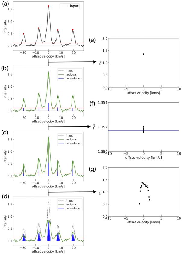
W33 in the KAGONMA survey                           1107
cluster may impact the types of stars formed (e.g. Bate 2009; Rumble       Table 1. A list of KAGONMA sources that have already been observed.
et al. 2015). In order to study the impact of radiative feedback, it is
important to investigate the effects and scales of star-forming regions    KAGONMA             l         b       v LSR (C18 O)a     Associated object
                                                                           name            [degrees] [degrees]      [km s−1 ]
of various evolutionary stages on the surrounding environment.
   There are several techniques to measure the temperature of the          KAG1             44.312      0.039       + 56.9        G044.3103 + 00.0416∗
interstellar medium (ISM). The dust temperature Tdust can be esti-         KAG35            14.613     −0.565       + 18.5          G14.628−0.572
mated by fitting a single-temperature greybody model to the observed       KAG39            14.565     −0.603       + 18.7          G14.555−0.606
                                                                           KAG45            14.454     −0.102       + 40.4         G014.481−00.109∗
spectral energy distribution (SED) of the dust continuum thermal
                                                                           KAG64            12.798     −0.202       + 35.6             W33 Main∗
emission (Hildebrand 1983). However, there are uncertainties in            KAG71           224.274     −0.833       + 18.0             CMa OB1
the assumptions of the dust emissivity coefficient κ and and dust          KAG72           201.446      0.638       + 6.5           G201.44 + 00.65
emissivity index β, which affect the accuracy of the derived dust          Notes.a Umemoto et al. (2017).
temperature. CO emission lines are commonly used for molecular             ∗
                                                                             H II region.
gas observations. In particular, the gas excitation temperature can
easily be obtained from the brightness temperature of 12 CO (J = 1–

                                                                                                                                                         Downloaded from https://academic.oup.com/mnras/article/510/1/1106/6481887 by guest on 19 January 2022
                                                                           de Geus & Blitz 1994), we catalogued 72 molecular cores/clumps
0) by assuming the optically thick and the filling factor in the           in part of the first and third quadrants of the Galactic plane (i.e.
observed beam is unity. However, it should be noted that the physical      10◦ ≤ l ≤ 50◦ and 198◦ ≤ l ≤ 236◦ , |b| ≤ 1◦ ). This catalogue
parameters in the centre of high-density cores may not reflect this, due   includes IRDCs, high-mass star-forming regions, and H II regions.
to optical thickness and freezing-out on to dust grains (e.g. Willacy,     We have already finished the mapping observations towards seven
Langer & Velusamy 1998; Tafalla et al. 2002; Christie et al. 2012;         cores or clumps, which are listed in Table 1. This work is the first
Feng et al. 2020).                                                         report of the KAGONMA survey project, which is an acronym
   NH3 has long been recognized as a good thermometer for the ISM          of Kagoshima Galactic Object survey with Nobeyama 45-metre
(Ho & Townes 1983) and its line observations have the advantage            telescope by Mapping in Ammonia lines. We present the results
of enabling us to derive physical parameters such as column density        for the W33 high-mass star-forming region, which is identified as
and optical depth from the splitting of the inversion transition into      KAGONMA 64.
hyperfine structure lines, with only reasonable assumptions that the          Fig. 1 shows the Spitzer -GLIMPSE 8.0-μm (Benjamin et al.
main transitions of the molecule are emitted under similar excitation      2003) image of the W33 region. W33 has six dust clumps defined in
conditions. The rotational temperature can also be estimated from          the Atacama Pathfinder Experiment (APEX) Telescope Large Area
the relationship between the intensity ratio of two different inversion    Survey of the GALaxy (ATLASGAL) 870-μm survey (Schuller et al.
transition lines and the optical depth. In addition, the inversion         2009; Contreras et al. 2013; Urquhart et al. 2014), which are W33
transitions in the lowest metastable rotational energy levels are easily   Main, W33 A, W33 B, W33 Main 1, W33 A1, and W33 B1 (see
excited in the typical temperatures of molecular clouds. Moreover,         Fig. 1). Immer et al. (2014) reported that these six dust clumps are at
NH3 molecules are abundant in the gas phase in cold and high-density       various stages (high-mass protostellar object, hot core, compact H II
environments (e.g. Bergin & Langer 1997; Tafalla et al. 2002).             region) in the star-forming process, based on their spectral energy
   Previous observational studies in NH3 lines have predominantly          distributions (SEDs) from centimetre to far-infrared. In Table 2, the
been single-beam pointings toward infrared dark clouds (IRDCs),            evolutionary stage of each dust clump is listed in order of earliest
young stellar objects (YSOs), and the centres of H II regions (e.g.        to latest. W33 Main harbours a compact H II region found by radio
Wilson, Batrla & Pauls 1982; Rosolowsky et al. 2008; Dunham et al.         continuum observations (Ho & Townes 1983), indicating massive star
2010; Urquhart et al. 2011; Wienen et al. 2018), and mappings at           formation. Water and methanol maser emission has been detected in
scales of a few parsec (e.g. Keto, Ho & Haschick 1987; Mangum,             W33 A, W33 Main, and W33 B (i.e. Haschick, Menten & Baan
Wootten & Mundy 1992; Toujima et al. 2011; Chibueze et al. 2013;           1990; Menten 1991; Immer et al. 2013), and OH maser sources have
Urquhart et al. 2015; Nakano et al. 2017; Billington et al. 2019; Burns    been detected in W33 A and W33 B (i.e. Caswell 1998; Colom et al.
et al. 2019). These studies have related the physical conditions of        2015).
active star-forming cores to the surrounding environment. Recently,           The distance to the W33 complex, based on annual parallax,
large surveys with the Green Bank Telescope (GBT) have been                was established as 2.4 kpc using VLBI water maser observations
conducted to study the relationship between the kinematics of              (Immer et al. 2013). W33 is located in the Scutum spiral arm of
dense gas and star formation in entire molecular clouds. These             the Milky Way. Some CO line observations covering the entire W33
observations cover giant molecular clouds (K-band Focal Plane Array        region were conducted (e.g. Stier et al. 1984; Sridharan et al. 2002;
(KFPA) Examinations of Young STellar Object Natal Environments             Kohno et al. 2018; Liu et al. 2021). Kohno et al. (2018) reported
(KEYSTONE): Keown et al. 2019), the Gould Belt star-forming                that W33 A, W33 Main, and W33 B1 are at a radial velocity of
regions (the Green Bank Ammonia Survey (GAS): Friesen et al.               ∼ 35 km s−1 and W33 B has a velocity of ∼ 58 km s−1 , while
2017) and the Galactic plane (the Radio Ammonia Mid-Plane Survey           Immer et al. (2013) reported that these clumps exist within a single
(RAMPS), covering 10◦ ≤ l ≤ 40◦ , |b| ≤ 0◦ .5: Hogge et al. 2018).         molecular cloud because these clumps have the same parallactic
These large surveys were made with the on-the-fly (OTF) mapping            distance.
mode. However, these unbiased surveys are rather shallow, since NH3           This work is organized as follows: in Section 2 we describe
line observations require a large amount of time to detect weaker          the set-up of our observations and data reduction. In Section 3
emission. Therefore, we conducted a high-sensitivity NH3 imaging           we present the results and estimated physical parameters of the
survey targeting dense molecular cores and the regions around them.        observed area. We evaluate the influence of star-formation feed-
   For our survey, we identified dense molecular cores based on the        back based on the rotational temperature distribution of NH3 lines
C18 O (J = 1–0) imaging data obtained as part of the FOREST (FOur-         in Section 4. In Section 5, we summarize our results and our
beam REceiver System on the 45m Telescope) Unbiased Galactic               conclusions.
plane Imaging survey with the Nobeyama 45-m telescope (FUGIN:
Umemoto et al. 2017). By using the clumpfind algorithm (Williams,

                                                                                                                 MNRAS 510, 1106–1117 (2022)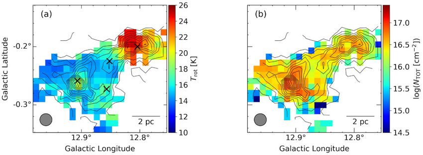
1108 T. Murase et al.
Downloaded from https://academic.oup.com/mnras/article/510/1/1106/6481887 by guest on 19 January 2022
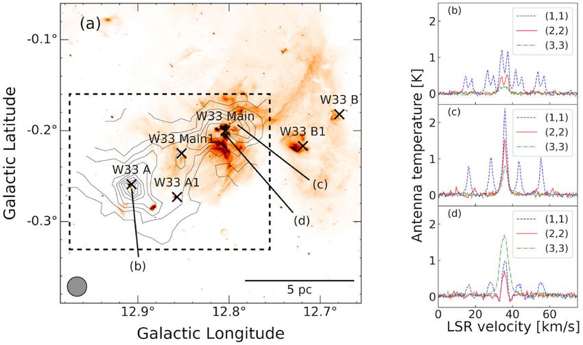
Figure 1. (a): The NH3 (1,1) integrated intensity map of the W33 complex in contours over the Spitzer-GLIMPSE 8.0-μm image. The lowest contour and
contour steps are 0.8 K km s−1 and 1.2 K km s−1 (30σ ), respectively. The cross marks indicate the dust clumps reported by the ATLASGAL 870-μm survey
(e.g. Contreras et al. 2013; Urquhart et al. 2014). The dashed rectangle shows our observing area. The NRO 45-m beamsize (FWHM) is indicated by the grey
circle shown in the lower left corner in panel (a). The (b)–(d) labels indicate the positions for the profiles shown in panels (b)–(d).
Table 2. Evolutionary stages of dust clumps.
Source l b Tex (C18 O)a Evolution stageb
[degrees] [degrees] [K]
W33 A1 12.857 −0.273 18 High-mass protostellar object
W33 B1 12.719 −0.217 23 High-mass protostellar object
W33 Main1 12.852 −0.225 19 High-mass protostellar object
W33 A 12.907 −0.259 18 Hot core
W33 B 12.679 −0.182 17 Hot core
W33 Main 12.804 −0.200 34 Compact H II region
Note.a Kohno et al. (2018), b Haschick & Ho (1983), Immer et al. (2014).
2 O B S E RVAT I O N S these correspond to a velocity coverage and resolution of 400 km
s−1 and 0.19 km s−1 , respectively. The telescope beam size was
2.1 NH3 and H2 O maser observations 75 arcsec at 23 GHz, which corresponds to 0.87 pc at 2.4 kpc. The
pointing accuracy was checked every hour using a known H2 O maser
We made mapping observations covering a 12 × 12 arcmin2 area
source, M16A at (α, δ)J2000 = (18h 15m 19s .4, −13◦ 46 30 .0), and was
including W33 A and W33 Main with the Nobeyama 45-m radio
better than 5 arcsec. The map centre was (l, b) = (12. 820, − 0.◦ 194).
◦
telescope from 2016 December–2019 April. We observed the NH3
The OFF reference position was taken at (l, b) = (13.◦ 481, +0.◦ 314),
(J,K) = (1,1), (2,2), (3,3), and H2 O maser lines simultaneously.
where neither C18 O (J = 1–0), NH3 , nor the H2 O maser was detected.
From 2019 February, we observed NH3 (3,3), (4,4), (5,5), and
We observed 280 positions using a 37.5-arcsec grid in equatorial
(6,6) lines at positions where the (3,3) emission line was detected
coordinates using the position switch method. For efficient obser-
(> 20σ ). The (3,3) emission line was observed again for relative
vation, three ON positions were set for each OFF position and
calibration. We used the H22 receiver, which is a cooled HEMT (High
integrations were repeated for 20 seconds at each position. To obtain
Electron Mobility Transistor) receiver, and the Spectral Analysis
uniform map noise, the scans were integrated until the root-mean-
Machine for the 45-m telescope (SAM45: Kuno et al. 2011), which
square (rms) noise level for each polarization of each observed line
is a digital spectrometer, to observe both polarizations for each
was reached to below 0.075 K. The typical system noise temperature,
line simultaneously. The bandwidth and spectral resolution were
Tsys , was between 100 and 300 K. The antenna temperature, Ta∗ , was
62.5 MHz and 15.26 kHz, respectively. At the frequency of NH3 ,
calibrated by the chopper wheel method (Kutner & Ulich 1981).
MNRAS 510, 1106–1117 (2022)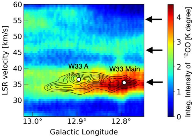
W33 in the KAGONMA survey                        1109
Table 3. Transition frequencies and excitation temperatures.                     the absorption of emission at the midway point. We will discuss the
                                                                                 absorption feature further in Section 4.3.
Transition                                Frequencya                Eu /kB a
                                            [GHz]                     [K]
                                                                                 3.2 Linewidth correlations
H2 O 612 –512 (maser)                      22.235080                    –
                                                                                 Fig. 3 shows the correlation plots of linewidths in the NH3
NH3   (1,1)                                23.694495                  23.3
NH3   (2,2)                                23.722633                  64.4       (1,1), (2,2), and (3,3) emission lines. In Fig. 3, we only used the
NH3   (3,3)                                23.870129                  123.5      observed positions where single-peak profiles were obtained (except
NH3   (4,4)                                24.139416                  200.5      for the enclosed positions in Fig. 2a). In our observations, the
NH3   (5,5)                                24.532988                  295.6      range of linewidths for each NH3 line was 2–6 km s−1 , which is
NH3   (6,6)                                25.056025                  408.1      broader than the expected thermal linewidth for temperatures in
Note.a From the JPL Submillimetre, Millimetre, and Microwave Spectral Line       W33 (approximately 0.2 km s−1 at a gas temperature of ∼ 20 K).
catalogue (Pickett et al. 1998). Eu is the energy of the upper level above the   These broader linewidths may be due to internal gas kinematic

                                                                                                                                                             Downloaded from https://academic.oup.com/mnras/article/510/1/1106/6481887 by guest on 19 January 2022
ground.                                                                          motions such as turbulence, outflows, and stellar winds. While the
                                                                                 linewidths of (1,1) and (2,2) emission show strong correlations, (3,3)
We summarize the parameters for the NH3 and H2 O maser line                      emission tends to have systematically broader linewidths than the
observations in Table 3.                                                         lower excitation transitions (see also fig. 11 in Urquhart et al. 2011).
                                                                                 As shown in Table 3, the NH3 (3,3) lines require approximately
                                                                                 five times higher excitation energies than (1,1) lines. Therefore, the
2.2 Data reduction                                                               emission regions of higher transitions of NH3 lines are considered
                                                                                 warmer and with more turbulent gas than (1,1) lines. These results
For data reduction, we use the Java NEWSTAR software package                     are similar to single-beam observations toward the centres of massive
developed by the Nobeyama Radio Observatory (NRO). Baseline                      young stellar objects (MYSOs) and H II regions (Urquhart et al. 2011;
subtraction was conducted individually for all spectra using a line              Wienen et al. 2018). Our results therefore show that such linewidth
function established using emission-free channels. By combining                  correlations in NH3 can also be seen on larger scales than the core
dual circular polarizations, the rms noise level was typically 0.04 K            scale.
at each position. A conversion factor of 2.6 Jy K−1 was used to
convert the antenna temperature to flux density.
   In this work, the intensities are presented as antenna temperature in         3.3 Deriving physical properties from NH3 lines
K. The NH3 lines have five hyperfine components, consisting of one
                                                                                 Using NH3 line profiles, we can derive several physical properties at
main line and four satellite lines. In our observations, these satellite
                                                                                 each observed position, such as optical depth, rotational temperature,
lines were detected only in the (1,1) transition. The number of map
                                                                                 and column density.
positions in which ≥3σ detections were achieved in (1,1), (2,2) and
                                                                                    Currently, there are two major methods for deriving the optical
(3,3) lines were 260, 231, and 172, respectively. No emission from
                                                                                 depth and rotational temperature (see Wang et al. 2020, for details).
transitions higher than (3,3) was detected.
                                                                                 They are known as the intensity ratio and hyperfine fitting methods.
   The NH3 profiles obtained in our observations can be categorized
                                                                                 The first method is derived from the intensity ratio between two
into three types (Figs 1b–d). Fig. 1(b) shows double-peak profiles
                                                                                 different excitation lines, assuming a Boltzmann distribution (e.g.
detected around W33 A. The double-peak profiles were detected at 46
                                                                                 Ho & Townes 1983; Mangum et al. 1992). The other method is
positions (the enclosure in Fig. 2a). The single-peak profiles shown
                                                                                 generating a model spectrum from the radiative transfer function
in Fig. 1(c) are typical NH3 profiles. The intensities of these two
                                                                                 and searching for parameters that match the observed profiles (e.g.
types of profile become weaker with higher excitation, while (3,3)
                                                                                 Rosolowsky et al. 2008; Urquhart et al. 2015). The common point
was detected more strongly than low-excitation lines of the centre of
                                                                                 in these methods is that the physical conditions along the velocity
W33 Main, where a compact H II region is located (Fig. 1d). In this
                                                                                 axis are assumed to be uniform. In general, however, molecular lines
region, we found absorption features at 33 and 39 km s−1 in (1,1)
                                                                                 have a velocity structure and the shape of profiles is asymmetric.
and (2,2) lines (see Section 4.3 for details).
                                                                                 Therefore, we used a method to derive physical parameters for
                                                                                 each velocity channel based on the intensity ratio method (see
3 R E S U LT S                                                                   Appendix A1 for more details).
                                                                                    The equation for deriving the optical depth and rotation tempera-
3.1 Spatial distribution of NH3 emission                                         ture using the intensity ratio method is described below. The optical
                                                                                 depth is derived from the line intensity ratios of the main and satellite
Fig. 2 shows the integrated intensity maps of the (1,1), (2,2), and              lines in the (1,1) transition (Ho & Townes 1983). The excitation
(3,3) lines in our observed region. The velocity range of each map is            energy differences between the hyperfine components are very small.
between 32.0 and 40.0 km s−1 . NH3 (1,1) emission is extended over               This allows us to assume that the main beam efficiencies, beam filling
a region of 12 × 12 arcmin2 , or 10 × 10 pc at 2.4 kpc. Two NH3                  factors, and excitation temperatures for all hyperfine components are
clumps were detected at W33 Main (l, b) = (12.◦ 804, − 0.◦ 200) and              identical. Therefore, we can use
W33 A (l, b) = (12.◦ 907, − 0.◦ 259).
                                                                                 Ta∗ (main)    1 − exp(−τ )
   Although maps of both the NH3 (1,1) and (2,2) lines show two                             =               ,                                         (1)
                                                                                 Ta∗ (sate)   1 − exp(−aτ )
peaks in W33 Main with a separation of about 2 arcmin, the (3,3)
map shows a single peak between them. After checking the profiles                where the values of a are 0.27778 and 0.22222 for the inner and outer
of the (1,1) and (2,2) lines there, we found hints of an absorption              satellite lines, respectively (Mangum et al. 1992).
signature. Therefore, the actual column density structure of W33                    Assuming that excitation conditions of gas emitting (1,1) and (2,2)
Main has only a single clump with an apparent gap inside caused by               lines were the same, the rotational temperature, Trot , can be estimated

                                                                                                                      MNRAS 510, 1106–1117 (2022)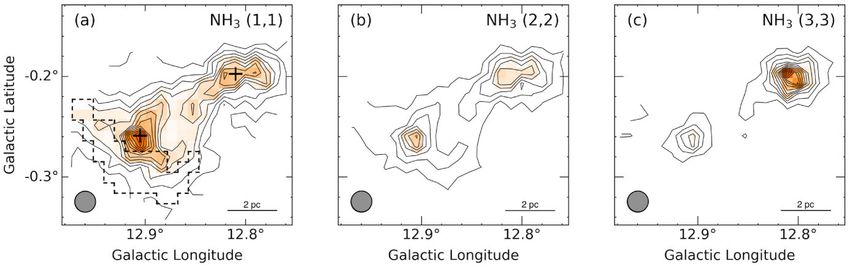
1110         T. Murase et al.

                                                                                                                                                                      Downloaded from https://academic.oup.com/mnras/article/510/1/1106/6481887 by guest on 19 January 2022
Figure 2. Integrated intensity map of NH3 : (a) (1,1), (b) (2,2), and (c) (3,3). The NRO45 beam size is indicated by the grey circle shown in the lower left corner
of each panel. The lowest contour and contour steps are 20σ (0.8 K km s−1 ) in Ta∗ , respectively. Plus marks indicate the positions of H2 O maser emission. The
black dashed enclosure shows the region where double-peak profiles were detected.

                                                                                    where kB is the Boltzmann constant, gJ is the rotational degeneracy,
                                                                                    gI is the nuclear spin degeneracy, gK is the K degeneracy, and E(J,
                                                                                    K) is the energy of the inversion state above the ground state.

                                                                                    3.4 Molecular gas properties
                                                                                    In this subsection, we will report the spatial distribution of the derived
                                                                                    physical parameters in W33 (Fig. 4), which were solved in each
                                                                                    velocity channel. The physical parameters at each position were
                                                                                    derived when the signal-to-noise ratios (S/N) of all peaks of NH3
                                                                                    (1,1) hyperfine components and the (2,2) main line are above 3σ .
                                                                                    The optical depth and rotational temperature errors were estimated
Figure 3 Scatter plots of FWHM linewidth of NH3 (1,1), (2,2), and (3,3)             to be ± 0.10 and ± 0.4 K, respectively (see Appendix A2).
emission. The solid lines indicate the line of equality.                               The derived optical depth ranges from 1 to 2, and its mean value
                                                                                    over all observed positions was 1.24 ± 0.10. The optical depth
                                                                                    distribution was not significantly different at each position.
from the intensity ratio of (2,2) to (1,1) and optical depth at each                   Maps of the rotational temperature and total column density are
observed position (Ho & Townes 1983), using                                         shown in Fig. 4. The range of rotational temperature was between 12
                                                                                    and 25 K (Fig. 4a). We found a clear difference between galactic east
                               −0.282
                                                                                    and west parts, corresponding to W33 A and W33 Main, respectively.
Trot (2, 2; 1, 1) = −41.1 ln
                                   τ (1, 1, m)                                      All pixels in W33 A were colder than 18 K, and most pixels in

                 Ta∗ (2, 2, m)                                                      W33 Main were warmer than 20 K. In our NH3 observations, the
  × ln 1 − ∗                   × [1 − exp(−τ (1, 1, m)]) ,       (2)                temperature change was a particularly noticeable characteristic. We
                 Ta (1, 1, m)
                                                                                    will discuss the relationship between the molecular gas temperature
where τ (1, 1, m) is the optical depth of the NH3 (1,1) main line.                  and star formation feedback in Section 4.2.
  Under local thermal equilibrium (LTE) conditions, the column                         The value of total column density ranges between 2 × 10¹⁵ and
density of NH3 in the (1,1) state can be estimated using the optical                8 × 1016 cm−2 , as shown in Fig. 4(b). The peak total column densities
depth, τ (1, 1, m), and the rotational temperature, Trot (Mangum et al.             of W33 Main and W33 A were (5.1 ± 0.1) × 1016 cm−2 and
1992):                                                                              (7.5 ± 0.1) × 1016 cm−2 , respectively. In contrast to the difference
                                                                                in the rotational temperature, there was no significant difference in
                                       Trot      v1/2
N (1, 1) = 2.78 × 10¹³ τ (1, 1, m)                        ,        (3)              the total column density between W33 Main and W 33 A. A weak
                                        K      km s−1                               dip in the measured column density at the centre of W33 main is
where v 1/2 is the velocity width, defined as the full width at half-               apparently due to the compact H II region.
maxmum (FWHM) of the main line. The column densities were
derived by using physical parameters at each observed position.
                                                                                    3.5 H2 O maser detection
When all energy levels are thermalized, the total column density,
NTOT (NH3 ), can be estimated by                                                    In our observations, H2 O maser emission was detected in W33 A
                                                                                  on 2017 May 21 at 26.3 Jy at (l, b) = (12.◦ 905, −0.◦ 257) and W33
NTOT (NH3 ) = N (1, 1)                                           (4)                Main on 2016 May 7 at 10.7 Jy at (l, b) = (12.◦ 811, −0.◦ 194). These
                             J   K                                                  masers are positionally consistent with those reported in the parallax

                         2gJ gI gK            Eu (J , K)                            observations of Immer et al. (2013). H2 O maser emission is believed
                 ×                 exp 23.3 −               ,
                             3                 kB Trot                              to be a signature of star formation in its early evolutionary stages (e.g.

MNRAS 510, 1106–1117 (2022)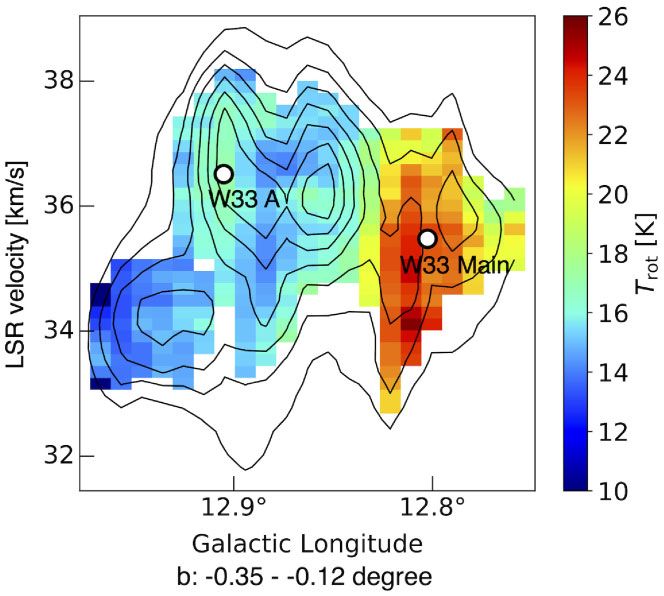
W33 in the KAGONMA survey                             1111

                                                                                                                                                                    Downloaded from https://academic.oup.com/mnras/article/510/1/1106/6481887 by guest on 19 January 2022
Figure 4. Spatial distributions of the physical parameters described in Section 3.3. The plotted values are representative along the velocity axis. (a) The
rotational temperature; (b) the total column density of NH3 gas. Contours indicate the NH3 (1,1) integrated intensity map, which is the same as in Fig. 2(a).
The NRO45 beam size is indicated by the grey circle shown in the lower left corner of each panel. Cross marks are the same as inside the dashed rectangle in
Fig. 1(a).

Figure 6. Longitude–velocity diagram of the 12 CO (J = 1–0) emission using
FUGIN data (colour image) and the NH3 (1,1) main line emission (contour).
The white circles indicate the peak velocities of W33 A and W33 Main in
the C18 O(J = 1–0) emission line (Umemoto et al. 2017; Kohno et al. 2018).
The arrows show the three velocity components at 35, 45, and 55 km s−1 .
                                                                                 Figure 5. The longitude–velocity diagram of the rotational temperature.
The lowest contour level and contour intervals are 0.06 K degree and 0.03 K
                                                                                 White circles, lowest contour level, and contour interval are same as in Fig. 6.
degree, respectively.

Sunada et al. 2007; Urquhart et al. 2011). Therefore, the detection              et al. 2018). On the other hand, the 45 km s−1 velocity component
indicates that both W33 A and W33 Main host star-forming activity.               shows weak emission extended over the wider W33 complex, and
                                                                                 its spatial distribution is not exclusively associated with the W33
                                                                                 complex. Kohno et al. (2018) concluded that the 45 km s−1 velocity
4 DISCUSSION
                                                                                 component is unrelated to star formation activity in the W33 complex.
                                                                                 Fig. 6 shows the longitude–velocity diagram using our data and
4.1 Velocity components in W33 complex
                                                                                 FUGIN 12 CO (J = 1–0) data2 integrated over Galactic latitudes
Kohno et al. (2018) and Dewangan, Baug & Ojha (2020) reported                    between −0.◦ 35 and −0.◦ 12, where contours indicate the NH3 (1,1)
three velocity components at 35, 45, and 55 km s−1 in the W33 region             main line. The dominant emission in CO and NH3 is detected at 35
from FUGIN CO survey data.1 The 35 km s−1 and 55 km s−1 velocity                 km s−1 and gas at this velocity is considered to be a molecular cloud
components exhibit similar spatial distributions (see fig. 5 in Kohno            related to the star formation activity in W33.

1 The55 km s−1 component is reported as 58 km s−1 in Kohno et al. (2018),
and 53 km s−1 in Dewangan et al. (2020).                                         2 http://jvo.nao.ac.jp/portal/nobeyama/

                                                                                                                           MNRAS 510, 1106–1117 (2022)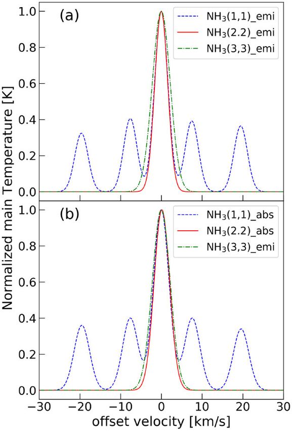
1112        T. Murase et al.
   Fig. 5 shows the longitude–velocity diagram of the our NH3 (1,1)       that there may be a relationship between the size of the heating area
data and rotational temperature. In the remainder of this work, we        and the properties of the heating source, although the continuum size
focus on the 35 km s−1 velocity component. Fig. 5 shows that there        of S252A is unknown. In order to make more certain statements about
are three velocity subcomponents centred on 35 km s−1 . In particular,    any possible relationship, observations of more regions are required.
we find that NH3 splits into two velocity components at W33 A (an            No temperature increase was obtained in W33 A, where strong
easternmost component at 34.5 km s−1 , and the main component of          NH3 emission was detected. In several previous studies, a large-
W33 A at 36.0 km s−1 ). These components with different velocities        scale outflow was reported in the centre of W33 A (Galván-Madrid
give rise to the double-peak profiles at positions shown in Fig. 2(a)     et al. 2010; Kohno et al. 2018). Using 12 CO(J=3–2) and (J = 1–0)
and have different properties, as shown below. From Fig. 1(b),            data, Kohno et al. (2018) investigated the intensity ratio, R3–2/1–0 ,
the intensity of the satellite lines differs between the two velocity     for the three velocity components at 35, 45, and 55 km s−1 . A
components, although the peak intensities of the NH3 (1,1) main line      high R3–2/1–0 was found in W33 A and W33 Main. These results
components are approximately the same. It suggests that the optical       are understood to be due to outflows from protostellar objects and
depths are different in these components, since the intensity ratio       heating by massive stars (Kohno et al. 2018). However, in our results,

                                                                                                                                                     Downloaded from https://academic.oup.com/mnras/article/510/1/1106/6481887 by guest on 19 January 2022
of the main and satellite lines depends on optical depth. The mean        the temperature distribution estimated by NH3 showed no evidence
optical depth of each velocity component was 1.39 (34.5 km s−1 ) and      of heating the molecular cloud around W33 A. We consider that
1.50 (36.0 km s−1 ), respectively. We also investigated temperature       gas heating by outflows is not effective, or else the size of the gas
differences between these two components. The emission at 34.5 km         heated by outflows in W33 A is significantly smaller than our beam
s−1 is colder than 16 K, while the 36.0 km s−1 component is at about      size (75 arcsec). High-resolution observations may be required to
18 K. However, within each velocity component, the temperature            investigate the impact of such stellar feedback in more detail.
is almost uniform (Fig. 6), suggesting there is no direct interaction
between these components. In addition, there was no change in the
                                                                          4.3 Comparison of emission and absorption components
temperature in the region between these two velocity components.
We obtained no evidence of interaction, such as collisions between        We tried to reproduce the profile shown in Fig. 1(d) using a
these components, in our observations. On the other hand, the NH3         combination of emission and absorption using a multi-component
emission associated with W33 Main at v LSR = 35 km s−1 is warmer          Gaussian profile with positive and negative peaks for each of the five
than 20 K and will be discussed further below.                            hyperfine lines in (1,1) and the main line in (2,2). Then we took the
                                                                          peak intensity, linewidth, and central velocity of each hyperfine line
                                                                          as free parameters. Fig. 7 shows our result for the (1,1)–(3,3) lines.
4.2 Star formation feedback traced by gas temperature
                                                                          In this result, the peak velocities of both components are consistent
In Section 3.4, we show that the temperature changes more signifi-        within the error.
cantly in the W33 complex than the other physical parameters. In this        High angular resolution observations toward W33 Main with the
section, we use the temperature distribution to discuss the influence     GBT, the Max Planck Institute for Radio Astronomy (MPIfR) 100-
range of star formation activity.                                         m radio telescope, and VLA also detected the absorption feature
   The rotational temperature in W33 Main is higher than in the           (Wilson et al. 1982; Keto & Ho 1989; Urquhart et al. 2011). NH3
other subcomponents (Figs 4a and 5). This suggests that embedded          gas in front of a bright continuum source is seen as an absorption
compact H II regions are having an impact on the physical conditions      feature (e.g. Keto et al. 1987; Henkel et al. 2008). The GBT profile
of the surrounding molecular gas. This feature of temperature             shows the absorption feature more clearly (see fig. A8 of Urquhart
distribution is also seen in some IRDCs, MYSOs, and H II regions          et al. 2011). This suggests that the size of the continuum sources
(Urquhart et al. 2015; Billington et al. 2019). Previous studies          is smaller than the beam size of the NRO 45-m. Interferometric
measuring molecular gas temperature have reported that quiescent          observations of the radio continuum also support our interpretation
regions exhibit temperatures of 10–15 K, while active star-forming        (e.g. Haschick & Ho 1983; Immer et al. 2014). However, in the (3,3)
regions associated with massive young stellar objects and H II regions    line, observations with either NRO 45-m, MPIfR, or GBT showed no
show temperatures higher than 20 K (e.g. Urquhart et al. 2015;            absorption feature. We will discuss this further in the next subsection.
Friesen et al. 2017; Hogge et al. 2018; Billington et al. 2019;              The decomposed line profiles show an interesting property in
Keown et al. 2019). In this study, observation points that measured       Fig. 7. Previous studies of NH3 lines have reported the combination
temperatures higher than 20 K are defined as the region under the         of absorption and emission lines with different peak velocities, such
influence of star-formation feedback.                                     as P Cygni or inverse P Cygni profiles, in all observed transitions
   Using Fig. 4(a), we estimated the size of the area influenced. The     (e.g. Wilson, Bieging & Downes 1978; Urquhart et al. 2011). In
projected area showing more than 20 K was estimated from the sum          W33 Main, the peak velocities of the emission and absorption
of the grid points (each of 37.5 × 37.5 arcsec2 = 0.19 pc2 ), resulting   exhibited consistent velocities within the errors (see the NH3 (1,1)
in a total size of 4.92 pc2 . Its equi-areal radius was 1.25 pc. The      and (2,2) spectra in Fig. 7). We also compared the linewidths of
apparent size of the compact H II region is 12.6 × 4.6 arcsec2 based      both components (Fig. 8). The absorption components in (1,1) and
on the 5-GHz continuum map obtained by White, Becker & Helfand            (2,2) lines show the same linewidth as the emission in the (3,3) line,
(2005) with the Very Large Array (VLA), which corresponds to              suggesting they originate in the same gas cloud. In many molecular
0.15 pc × 0.05 pc at 2.4 kpc. The heated area is several times larger     cores, the higher transitions of NH3 emission lines are thought to be
than the compact H II region.                                             emitted from more compact regions and also show broader linewidths
   In a previous study by our group, we investigated the size of a        (Urquhart et al. 2011, see also Section 3.2 of this work). Our results
molecular gas cloud affected by the H II region at the edge of the        may indicate that the absorption component traces more turbulent
Monkey Head Nebula (MHN: Chibueze et al. 2013). They reported             gas close to the continuum sources.
no apparent impact of the extended H II region of the MHN. However,          Because an absorption feature delineates the physical properties
the molecular gas around the compact H II region S252A has higher         of gas in front of a continuum source, it can be used to separate the
temperatures and the size of the heating area was 0.9 pc. We expect       physical properties along the line of sight and within an observed

MNRAS 510, 1106–1117 (2022)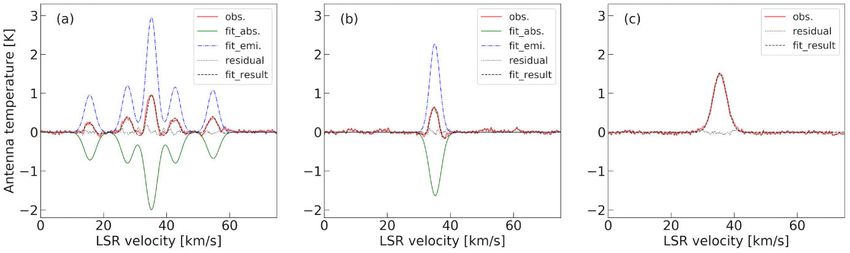
W33 in the KAGONMA survey                            1113

                                                                                                                                                                      Downloaded from https://academic.oup.com/mnras/article/510/1/1106/6481887 by guest on 19 January 2022
Figure 7. The profile in Fig. 1(d) is reproduced by a multi-component Gaussian. Fit results for (a) the NH3 (1,1) profile, (b) the (2,2) profile, and (c) the (3,3)
profile. The blue dash–dotted lines, green lines, red lines, and black dashed lines indicate the observed profile, absorption component, emission component, and
fitting result profile, respectively. The dotted lines show the residual profile in the same colour. Since no absorption feature was found in the (3,3) profile, we
apply only an emission component.

                                                                                    the error. This suggests that the physical conditions of the NH3 gas
                                                                                    surrounding the continuum sources are the same. Therefore, the H II
                                                                                    region located in the centre of W33 Main may still be embedded
                                                                                    in dense molecular gas with the same motion as the surrounding
                                                                                    environment.

                                                                                    4.4 Absence of absorption in NH3 (3,3)
                                                                                    An absorption feature must be located in front of a continuum
                                                                                    background and be affected by its brightness. As mentioned in
                                                                                    Section 4.3, the continuum source size is smaller than the beam size
                                                                                    of the NRO 45-m. Previous studies have reported objects that show
                                                                                    P Cygni and inverse P Cygni profiles in all inversion transitions
                                                                                    in NH3 (e.g. Wilson et al. 1978; Burns et al. 2019). In models
                                                                                    assuming a spherically symmetric molecular gas cloud with the
                                                                                    continuum source at its centre, these features can reveal the expansion
                                                                                    or contraction of gas in front of the continuum source. The emission
                                                                                    and absorption features of NH3 (1,1) and (2,2) lines obtained in
                                                                                    our observations are detected with the same line-of-sight velocity.
                                                                                    However, for the (3,3) transition, only the emission component was
                                                                                    detected, without any hint of absorption. We tried to explain all
                                                                                    transition profiles in our observations consistently, but failed under
                                                                                    the spherically symmetric model after considering the following
                                                                                    three possibilities.
                                                                                       An absorption feature requires a bright continuum background.
                                                                                    Therefore, we estimated the brightness temperature of the H II region
                                                                                    in W33 Main using an electron temperature and emission measure
                                                                                    of 7800 K and 1.5 × 10⁶ pc cm−6 from observations at 15.375 GHz
                                                                                    with the National Radio Astronomy Observatory (NRAO) 140-
                                                                                    foot telescope (Schraml & Mezger 1969). The expected brightness
                                                                                    temperature of the continuum emission at our observed frequency,
Figure 8. Comparison of the emission and absorption components obtained             Tcont , is calculated to be about 6 K, which is sufficient to produce
by Gaussian fitting. The horizontal axis indicates the offset velocity from         an absorption feature. Since absorption features are detected in both
the central velocity of each transition main line. The vertical axis shows the      (1,1) and (2,2) lines, and since NH3 inversion transitions are detected
relative intensity normalized by each main line peak. (a) NH3 (1,1)–(3,3)           in a narrow frequency range, the continuum brightness temperature
emission profiles; (b) comparison between the negative-intensity profiles of        is almost the same for all observed NH3 lines. The value of Tcont at
the absorption components of (1,1) and (2,2) and the positive-intensity profile
                                                                                    the frequency of NH3 (3,3) is therefore also strong enough to produce
of (3,3).
                                                                                    an absorption feature.
beam. The estimated optical depth and rotational temperature are τ                     The spatial distribution of the NH3 gas observed in the (3,3)
= 0.89 ± 0.10 and Trot = 20.9 ± 0.4 K in the emission component, τ                  line may differ from that of other lines. If no NH3 gas for
= 0.91 ± 0.10 and Trot = 21.1 ± 0.4 K in the absorption component.                  producing absorption is located in front of the continuum source,
The physical parameters of the two components are the same within                   we would not observe any absorption feature, which contradicts

                                                                                                                            MNRAS 510, 1106–1117 (2022)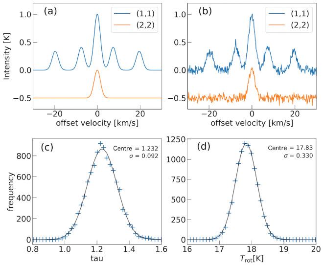
1114        T. Murase et al.
the detection of absorption features at NH3 (1,1) and (2,2). It is       Observatory, a branch of the National Astronomical Observatory
unlikely that the distributions of the same molecular species are        of Japan. This publication makes use of data from FUGIN, FOREST
vastly different at different excitation levels. Wilson et al. (1982)    Unbiased Galactic plane Imaging survey with the Nobeyama 45-m
observed the centre of W33 Main with the MPIfR 100-m radio               telescope, a legacy project in the Nobeyama 45-m radio telescope.
telescope in the NH3 (1,1), (2,2), (3,3), and (4,4) lines. They          This study used ASTROPY, a Python package for Astronomy (Astropy
detected absorption features only in para-NH3 lines (see fig. 1 of       Collaboration et al. 2013, 2018), APLPY, a Python open-source pack-
Wilson et al. 1982). They also failed to explain the absence of          age for plotting (Robitaille 2019), MATPLOTLIB, a Python package
absorption in the (3,3) line under an LTE assumption in all four         for visualization (Hunter 2007), NUMPY, a Python package for sci-
levels, even when considering two molecular clouds with different        entific computing (Harris et al. 2020), and Overleaf, a collaborative
temperatures.                                                            tool.
   NH3 maser emission is another possibility. The NH3 (3,3) maser           Part of this work was carried out under the common use observa-
has been detected in star-forming regions (e.g. W51: Zhang & Ho          tion programme at Nobeyama Radio Observatory (NRO).
1995; G030.7206−00.0826: Urquhart et al. 2011; G23.33−0.30:

                                                                                                                                                          Downloaded from https://academic.oup.com/mnras/article/510/1/1106/6481887 by guest on 19 January 2022
Walsh et al. 2011, Hogge et al. 2019), and has been reported to
                                                                         DATA AVA I L A B I L I T Y
have a narrow linewidth. Wilson et al. (1982) proposed a similar
model: only (3,3) in a state of population inversion. However, this      The NH3 data underlying this article will be shared on reasonable
requires coincidental masking of the absorption component by maser       request to the corresponding author.
emission over the full velocity width, because the (3,3) emission line
has a linewidth the same as or broader than the thermal excitation
line of NH3 (1,1) and (2,2) lines, as shown in Fig.8. Therefore, this    REFERENCES
possibility is not realistic.                                            Astropy Collaboration et al.2013, A&A, 558, A33
   High angular resolution and high-sensitivity multi-transition NH3     Astropy Collaboration et al., 2018, AJ, 156, 123
observations are required to investigate an explanatory model in more    Bate M. R., 2009, MNRAS, 392, 1363
detail. This should be possible with the Square Kilometre Array          Bate M. R., Keto E. R., 2015, MNRAS, 449, 2643
(SKA) and next-generation Very Large Array (ngVLA).                      Benjamin R. A. et al., 2003, Publ. Astron. Soc. Aust, 115, 953
                                                                         Bergin E. A., Langer W. D., 1997, ApJ, 486, 316
                                                                         Billington S. J., Urquhart J. S., Figura C., Eden D. J., Moore T. J. T., 2019,
5 CONCLUSIONS                                                                MNRAS, 483, 3146
                                                                         Burns R. A. et al., 2019, PASJ, 71, 91
We performed mapping observations toward the W33 high-mass star-         Caswell J. L., 1998, MNRAS, 297, 215
forming region in NH3 (1,1), (2,2), (3,3), and H2 O maser transitions    Chibueze J. O. et al., 2013, ApJ, 762, 17
using the Nobeyama 45-m radio telescope. Our observations detected       Christie H. et al., 2012, MNRAS, 422, 968
only a single velocity component around 35 km s−1 . NH3 (1,1)            Colom P., Lekht E. E., Pashchenko M. I., Rudnitskij G. M., 2015, A&A, 575,
and (2,2) lines are extended over the observed region. From these            A49
observations, the distribution of the physical parameters of the         Contreras Y. et al., 2013, A&A, 549, A45
                                                                         Deharveng L. et al., 2012, A&A, 546, A74
dense molecular gas was obtained. Consequently, the molecular gas
                                                                         Deharveng L. et al., 2015, A&A, 582, A1
surrounding the H II region located at W33 Main was found to exhibit     Dewangan L. K., Baug T., Ojha D. K., 2020, MNRAS, 496, 2
a higher temperature (> 20 K) than the rest of the observed area. The    Dunham M. K. et al., 2010, ApJ, 717, 1157
size of the influence area is estimated at approximately 1.25 pc. The    Duronea N. U., Cappa C. E., Bronfman L., Borissova J., Gromadzki M., Kuhn
heating source of the molecular gas is considered to be the compact          M. A., 2017, A&A, 606, A8
H II region in W33 Main. Strong NH3 emission was also detected in        Feng S. et al., 2020, ApJ, 901, 145
W33 A; however, no temperature increase in its molecular gas was         Friesen R. K. et al., 2017, ApJ, 843, 63
obtained.                                                                Galván-Madrid R., Zhang Q., Keto E., Ho P. T. P., Zapata L. A., Rodrı́guez
   Molecular gas in front of the compact H II region in W33 Main             L. F., Pineda J. E., Vázquez-Semadeni E., 2010, ApJ, 725, 17
was detected as an absorption feature. Gaussian fitting of the           Goldsmith P. F., 2001, ApJ, 557, 736
                                                                         Harris C. R. et al., 2020, Nature, 585, 357
emission and absorption components reveals that the peak velocities
                                                                         Haschick A. D., Ho P. T. P., 1983, ApJ, 267, 638
of both components are almost the same. This suggests that the           Haschick A. D., Menten K. M., Baan W. A., 1990, ApJ, 354, 556
continuum source located in the centre of W33 Main may still be          Hatchell J. et al., 2013, MNRAS, 429, L10
embedded in the dense molecular gas. Curiously, the absorption           Henkel C., Braatz J. A., Menten K. M., Ott J., 2008, A&A, 485, 451
feature was detected only in the NH3 (1,1) and (2,2) transitions but     Hennebelle P., Chabrier G., 2011, ApJ, 743, L29
not in the (3,3) transition. We tried to explain these NH3 profiles      Hennebelle P., Commerc¸on B., Lee Y.-N., Chabrier G., 2020, ApJ, 904, 194
using spherically symmetric models but concluded that no simple          Hildebrand R. H., 1983, QJRAS, 24, 267
model could explain the observed profiles in all three transitions       Ho P. T. P., Townes C. H., 1983, ARA&A, 21, 239
towards W33 Main. It is possible that the spatial distributions of       Högbom J. A., 1974, A&AS, 15, 417
the NH3 (3,3) emitting region and the continuum sources may be           Hogge T. et al., 2018, ApJS, 237, 27
                                                                         Hogge T. G. et al., 2019, ApJ, 887, 79
different.
                                                                         Hunter J. D., 2007, Computing in Science & Engineering, 9, 90
                                                                         Immer K., Galván-Madrid R., König C., Liu H. B., Menten K. M., 2014,
                                                                             A&A, 572, A63
AC K N OW L E D G E M E N T S
                                                                         Immer K., Reid M. J., Menten K. M., Brunthaler A., Dame T. M., 2013,
We thank the Nobeyama Radio Observatory staff members (NRO) for              A&A, 553, A117
their assistance and observation support. We also thank the students     Kennicutt R. C., 2005, in Cesaroni R., Felli M., Churchwell E., Walmsley
of Kagoshima University for their support during the observations.           M., eds, IAU Symp. Vol. 227, Massive Star Birth: A Crossroads of
                                                                             Astrophysics. Cambridge University Press,Cambridge, p. 3
The 45-m radio telescope is operated by the Nobeyama Radio

MNRAS 510, 1106–1117 (2022)
W33 in the KAGONMA survey 1115
Keown J. et al., 2019, ApJ, 884, 4 A1 The ‘CLEAN’ procedure for an NH3 profile
Keto E. R., Ho P. T. P., 1989, ApJ, 347, 349
Keto E. R., Ho P. T. P., Haschick A. D., 1987, ApJ, 318, 712 In many investigations using NH3 , the integrated or peak intensity
Kohno M. et al., 2018, PASJ, 70, S50 of lines is used to derive the gas physical parameters. However,
Krieger N. et al., 2017, ApJ, 850, 77 for objects with velocity structure this procedure may not be
Krumholz M. R., McKee C. F., Bland-Hawthorn J., 2019, ARA&A, 57, ideal, because of the non-linearity of the equations in derivation.
227 Therefore, we should estimate the physical parameters in each
Kuno N. et al., 2011, in proc. 2011 XXXth URSI General Assembly and velocity component first.
Scientific Symposium IEEE, New York, p. 1 In this subsection, we describe our method used in this work to
Kutner M. L., Ulich B. L., 1981, ApJ, 250, 341 derive the physical parameters based on the CLEAN algorithm. The
Lada C. J., Lada E. A., 2003, ARA&A, 41, 57
CLEAN algorithm was devised by Högbom (1974) and is the most
Liu X.-L., Xu J.-L., Wang J.-J., Yu N.-P., Zhang C.-P., Li N., Zhang G.-Y.,
2021, A&A, 646, A137
used iterative method to improve radio interferometer images. In
Mangum J. G., Wootten A., Mundy L. G., 1992, ApJ, 388, 467 general, CLEAN is used in a two-dimensional map with a fixed dirty
Menten K. M., 1991, ApJ, 380, L75 beam over the whole imaging field. In our method, we assumed that
Downloaded from https://academic.oup.com/mnras/article/510/1/1106/6481887 by guest on 19 January 2022
Nakano M. et al., 2017, PASJ, 69, 16 the detected intensities of each channel are a Dirac delta function for
Paron S., Granada A., Areal M. B., 2021, MNRAS, 505, 4813 each velocity component. However, the NH3 inversion transition line
Pickett H. M., Poynter R. L., Cohen E. A., Delitsky M. L., Pearson J. C., exhibits a hyperfine structure and the observed five-line intensities
Müller H. S. P., 1998, J. Quant. Spec. Radiat. Transf., 60, 883 depend on the optical depth. We employ the hyperfine structure
Robitaille T., 2019, APLpy v2.0: The Astronomical Plotting Library in pattern with an optical depth as the dirty beam for each delta-function
Python, Zenodo, doi: component.
Rosolowsky E. W., Pineda J. E., Foster J. B., Borkin M. A., Kauffmann J.,
Our method is composed of the following six steps (Fig. A1).
Caselli P., Myers P. C., Goodman A. A., 2008, ApJS, 175, 509
(i) Find the peak intensity and velocity of the main line from the
Rumble D. et al., 2015, MNRAS, 448, 1551
Rumble D. et al., 2016, MNRAS, 460, 4150 input profile (Fig. A1a). The frequency and corresponding velocity
Rumble D., Hatchell J., Kirk H., Pattle K., 2021, MNRAS, 505, 2103 offsets between the NH3 (1,1) main line and the other four satellite
Schraml J., Mezger P. G., 1969, ApJ, 156, 269 lines are fixed as shown in Table A1. This can give the five hyperfine
Schuller F. et al., 2009, A&A, 504, 415 line intensities (indicated as red points in Fig. A1a). From this dataset,
Seifried D., Sánchez-Monge Á., Suri S., Walch S., 2017, MNRAS, 467, the four intensity ratios between the main line and satellite lines are
4467 obtained.
Shimajiri Y., Takahashi S., Takakuwa S., Saito M., Kawabe R., 2008, ApJ, (ii) Estimate the optical depth using each intensity ratio following
683, 255 equation (1). To get the optical depth for a single velocity component,
Sridharan T. K., Beuther H., Schilke P., Menten K. M., Wyrowski F., 2002,
we take the median of the estimated four optical depths (black dots
ApJ, 566, 931
in Fig. A1e).
Stier M. T. et al., 1984, ApJ, 283, 573
Sunada K., Nakazato T., Ikeda N., Hongo S., Kitamura Y., Yang J., 2007,
(iii) Using the estimated optical depth and the main line intensity
PASJ, 59, 1185 after step (ii), reproduce the intensity of each satellite line.
Tafalla M., Myers P. C., Caselli P., Walmsley C. M., Comito C., 2002, ApJ, (iv) Subtract the scaled reproduced main and satellite lines from
569, 815 the original profile. We call the scaling factor of the reproduction the
Thompson M. A., Urquhart J. S., Moore T. J. T., Morgan L. K., 2012, MNRAS, gain factor G < 1 (indicated as blue bars in Fig. A1b). This gain
421, 408 factor corresponds to the loop gain in the CLEAN algorithm. In this
Toujima H., Nagayama T., Omodaka T., Handa T., Koyama Y., Kobayashi work, we adopted a gain factor of 0.2.
H., 2011, PASJ, 63, 1259 (v) Steps (ii)–(iv) are iterated until one of the five hyperfine
Tursun K. et al., 2020, A&A, 643, A178 intensities falls below a 3σ noise level (Fig. A1c). In one velocity
Umemoto T. et al., 2017, PASJ, 69, 78
channel, it is typically iterated 3–5 times. The resultant profile is used
Urquhart J. S. et al., 2011, MNRAS, 418, 1689
Urquhart J. S. et al., 2014, A&A, 568, A41
as the input profile in step (i) (the blue horizontal line in Fig. A8f
Urquhart J. S. et al., 2015, MNRAS, 452, 4029 shows the median value of the optical depth for a channel).
Urquhart J. S., Thompson M. A., Morgan L. K., Pestalozzi M. R., White G. (vi) Steps (i)–(v) are iterated n times for the subtracted profile. We
J., Muna D. N., 2007, A&A, 467, 1125 recommend limiting the velocity range to the main line and searching
Walsh A. J. et al., 2011, MNRAS, 416, 1764 for the peak intensity (which corresponds to cleanbox in CLEAN).
Wang S., Ren Z., Li D., Kauffmann J., Zhang Q., Shi H., 2020, MNRAS, These steps (i)–(v) continue until the peak intensity of the residual
499, 4432 main line is below a 3σ noise level (Fig. A1d).
Ward-Thompson D. et al., 2007, PASP, 119, 855
White R. L., Becker R. H., Helfand D. J., 2005, AJ, 130, 586 Figs A1(d) and (g) show the final resulting profile and optical depth
Wienen M., Wyrowski F., Menten K. M., Urquhart J. S., Walmsley C. of each velocity channel. Using the optical depths and the intensity
M., Csengeri T., Koribalski B. S., Schuller F., 2018, A&A, 609, ratio of NH3 (1,1) and (2,2) for each velocity channel, the rotational
A125 temperature can be estimated.
Willacy K., Langer W. D., Velusamy T., 1998, ApJ, 507, L171
Williams J. P., de Geus E. J., Blitz L., 1994, ApJ, 428, 693
Wilson T. L., Batrla W., Pauls T. A., 1982, A&A, 110, L20
A2 Error estimation by the Monte Carlo method
Wilson T. L., Bieging J., Downes D., 1978, A&A, 63, 1
Zhang Q., Ho P. T. P., 1995, ApJ, 450, L63 Evaluating the error of observed parameter estimation is important.
Although the error is straightforward when calculating the value from
APPENDIX A: TECHNICAL DESCRIPTION
U S E D T O E S T I M AT E T H E P H Y S I C A L
PA R A M E T E R S
MNRAS 510, 1106–1117 (2022)1116 T. Murase et al.
Downloaded from https://academic.oup.com/mnras/article/510/1/1106/6481887 by guest on 19 January 2022
Figure A1. The workflow of our method, based on an observation position at (l, b) = (12.801, −0.196). Panels (a)–(d) and (e)–(g) show the profiles and the
estimated optical depth in each step, respectively. The red line in panels (a)–(d) indicates the 3σ level. See the main text for further detail.
direct measurement, an indirect parameter derived through non-linear used an optical depth value of 1.24 (the average value across the
equations is complicated. Instead of non-linear error propagation W33 complex). The peak intensity of the (1,1) main line was 1.0
analysis, we used a Monte Carlo method in this work. For the sample (Fig. A2a). For the (2,2) data, we used a Gaussian profile with half
data of NH3 (1,1), we adopt a noise-free Gaussian profile assuming the intensity of the (1,1) emission. Using equation (2), the value of the
a constant optical depth in the line-of-sight direction. Here, we rotational temperature was derived to be 17.83 K adopting τ = 1.24
MNRAS 510, 1106–1117 (2022)W33 in the KAGONMA survey 1117
Table A1. The velocity offset between the main line and four satellite lines in NH3 (1,1)
(Krieger et al. 2017; Ho & Townes 1983).
Transition F1 = 0 → 1 F1 = 2 → 1 F1 = 1 → 1 F1 = 1 → 2 F1 = 1 → 0
2→2
Offset [MHz] 0.92 0.61 0 −0.61 -0.92
Offset [km −19.48 −7.46 0 7.59 19.61
s−1 ]
Downloaded from https://academic.oup.com/mnras/article/510/1/1106/6481887 by guest on 19 January 2022
Figure A2. The result of error estimation with our method. (a) Model profiles of NH3 (1,1) (blue) and (2,2) (orange); (b) profiles with Gaussian noise (rms
0.04 K) added to the model profile shown in (a); (c) and (d) frequency distributions of the optical depth and rotational temperature, respectively. The black line
shows the best-fitting log–normal function.
and R(2, 2)/(1, 1) = 0.5. The linewidths of (1,1) and (2,2) profiles were temperature for the samples were 0.092 and 0.330 K, respectively.
assumed to be the same. We added Gaussian noise (σ noise 0.04) to In this work, we determined the errors of these physical parameters
these profiles and sampled 105 times. as ± 0.10 and ± 0.4 K, respectively.
Figs A2(c) and (d) show histograms of the distributions of the
sampled optical depth and rotational temperature, respectively. These This paper has been typeset from a TEX/LATEX file prepared by the author.
distributions are close to Gaussian (black lines in Figs A2c and d).
The standard deviations of the resultant optical depth and rotational
MNRAS 510, 1106–1117 (2022)You can also read