Lattice Boltzmann Multicomponent Model for Direct-Writing Printing
←
→
Page content transcription
If your browser does not render page correctly, please read the page content below
Lattice Boltzmann Multicomponent Model for Direct-Writing Printing
                                                               Michele Monteferrante,1, a) Andrea Montessori,1 Sauro Succi,1, 2, 3 Dario Pisignano,4, 5 and Marco Lauricella1, b)
                                                               1)
                                                                  Istituto per le Applicazioni del Calcolo CNR, Via dei Taurini 19, 00185 Rome,
                                                               Italy
                                                               2)
                                                                  Center for Life Nano Science@La Sapienza, Istituto Italiano di Tecnologia, 00161 Roma,
                                                               Italy
                                                               3)
                                                                  Harvard Institute for Applied Computational Science, Cambridge, Massachusetts,
                                                               United States
                                                               4)
                                                                  Dipartimento di Fisica, Università di Pisa, Largo B. Pontecorvo 16 3, 56127 Pisa,
                                                               Italy
                                                               5)
                                                                  NEST, Istituto Nanoscienze-CNR, Piazza S. Silvestro 12, 56127 Pisa, Italy
                                                               We introduce a mesoscale approach for the simulation of multicomponent flows to model the direct-writing
arXiv:2102.02655v1 [physics.flu-dyn] 4 Feb 2021

                                                               printing process, along with the early stage of ink deposition. As an application scenario, alginate solutions
                                                               at different concentrations are numerically investigated alongside processing parameters, such as apparent
                                                               viscosity, extrusion rate, and print head velocity. The present approach offers useful insights on the ink
                                                               rheological effects upon printed products, susceptible to geometric accuracy and shear stress, by manufacturing
                                                               processes such as the direct-writing printing for complex photonic circuitry, bio-scaffold fabrication, and tissue
                                                               engineering.

                                                  I.   INTRODUCTION

                                                     In the last decade, 3D printing processes have gained enormous attention as tool for additive manufacturing in many
                                                  fields of science and engineering. The major success of 3D printing is mostly due to the digital process control, which
                                                  offers remarkable flexibility in terms of patterning through material deposition. By exploiting a computer-controlled
                                                  layer-by-layer fabrication technique, soft materials are utilised in fused deposition modelling and in extrusion direct-
                                                  writing bio-plotters that apply a pressure gradient to fluids, possibly generating architected matter with qualitatively
                                                  new properties1,2 . As a consequence, this set of technologies is nowadays exploited in a wide variety of applications,
                                                  such as tissue engineering (e.g., bio-compatible scaffolds), microsystems (lab-on-chip), microelectronics (sensors), and
                                                  aerospace structures (aircraft engine bracket), to name a few3–5 . The vast potential of additive manufacturing requires,
                                                  however, an unprecedented control over several aspects of the soft materials involved in the 3D printing process. Their
                                                  dynamics, composition, structure, function and rheology are all key elements, which severely affect the features of the
                                                  finally produced parts and structures.
                                                     In this framework, efficient numerical simulations might offer a crucial help to understand the relevant, and in-
                                                  terplaying, characteristics of the fluids and experimental setups, similarly to other manufacturing processes where
                                                  computational tools have been successfully applied in the last two decades (e.g. electrospinning6 , electrospray7 ). In
                                                  the direct-writing printing context, numerical simulations could be used to maximise the printability of a given ink,
                                                  avoid process failures and anticipate the microstructural properties of the products, by providing a set of observables
                                                  (e.g., flow rate, stress tensor), which are often difficult to access experimentally. Printability is usually studied em-
                                                  pirically, and a priori criteria are not available that, given an ink and a prototype model, allow the success of the
                                                  manufacturing process to be reliably predicted. Moreover, the challenging characteristic length scale of the process,
                                                  i.e. the diameter of the print head nozzle used to deposit materials, significantly constrain the possible choices within
                                                  available computational methods. For instance, microscopic techniques, such as molecular dynamics, are generally
                                                  unable to access length and time scales of experimental relevance, for want of computing resources. On the other
                                                  hand, finite volume or finite element methods may also become computationally expensive in the presence of moving
                                                  boundary conditions, such as the ones describing the moving print head.
                                                     Mesoscale techniques, and particularly the Lattice Boltzmann (LB) method8–10 offer an appealing alternative to
                                                  both methods above, eventually striking an optimal balance between the two. Indeed LB moves noise-free discrete
                                                  probability distributions along force-free (straight) trajectories and represents the effect of molecular collisions through
                                                  the relaxation towards a suitable lattice local-equilibrium. Once the lattice symmetry and the local equilibria are
                                                  suitably designed, the scheme can be shown to reproduce quantitatively the Navier-Stokes equations of fluid flows.
                                                  The result is a very elegant and efficient computational scheme, featuring outstanding amenability to parallel imple-
                                                  mentations also in the presence of strong nonlinearities and complex boundary conditions8,9,11 .

                                                  a) First   author
                                                  b) Corresponding    author: m.lauricella@iac.cnr.it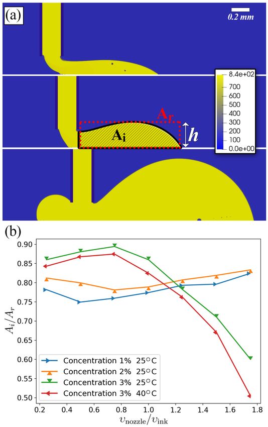
2

   In this work, we open a new route for predicting 3D printability, developing the regularised version of the Colour
Gradient (CG) Lattice Boltzmann (LB) model8–10 to account for the Non-Newtonian rheological behaviour, typical
of 3D printed pseudo-plastic inks. These systems endure a largely varying apparent viscosity, depending on the shear
rate12 . The regularised version of the LB method mitigates issues related to both low and high viscosities13 , the first
threatening numerical stability, while the latter undermining the very hydrodynamic limit of the LB scheme. Further,
the shift in the nozzle position during actual 3D printing processes is also included. As a practical application, we
focus on sodium alginate solutions, which are widely used in direct-writing printing to manufacture scaffolds for cell
cultures and tissue regeneration4 . The printing accuracy is discussed in terms of a Parameter Optimization Index
(POI)14 , which is predicted in terms of the numerical inputs.

II.   MODEL DETAILS

A.    Regularized colour-gradient lattice Boltzmann model

  The regularized CG method for multicomponent-multiphase systems provides computationally efficient access to
capillary number regimes relevant to microfluidics15 .
  The general form of CG LB equations10,16,17 writes as follows:

                                       fik (~x + ~ci ∆t, t + ∆t) = fik (~x, t) + Ωki [fik (~x, t)],                           (1)

where k is the colour component, i is the index spans the lattice discrete directions, and Ωki denotes the collision
operator of the Colour Gradient model. In Eq. 1, fik , represents the probability of finding a particle of the k − th
component at position ~x and time t with discrete lattice velocity ~ci . For the sake of simplicity, we adopt the standard
D2Q9 lattice, and only two colours are assumed in the system, i.e. yellow and blue, standing for the dense ink and air,
respectively. In the following, i = 0 denotes the resting population with zero velocity, while i ∈ √  [1, . . . , 8] represent the
directions at angle θ = (i − 1)π/4 with velocity modulus |~ci | = 1 for i ∈ [1, 3, 5, 7], and |~ci | = 2 for i ∈ [2, 4, 6, 8] in
lattice units, assumed ∆xLB = 1 and ∆tLB = 1. A comparison among the regularized version of the Colour Gradient
(CG) lattice Boltzmann (LB) model15 and other LB diffuse interface approaches (e.g., pseudo-potential model, free
energy model) was discussed by S. Leclaire and coworkers18 . The density, ρk , of the k − th fluid component is assessed
as the zeroth moment of the distribution functions
                                                             X
                                                ρk (~x, t) =    fik (~x, t) ,                                                  (2)
                                                                       i

while the total momentum, ρ~u, is defined by the first order moment:
                                                             XX
                                                     ρ~u =             fik (~x, t) ~ci ,                                      (3)
                                                              k    i

being ρ the sum of the two component densities. The collision operator, Ωki , results from the combination of three
sub-operators:

                                                Ωki = (Ωki )(3) [(Ωki )(1) + (Ωki )(2) ].                                     (4)

The first, (Ωki )(1) , is the standard BGK operator:

                                                          1
                                             (Ωki )(1) = − [fik (~x, t) − fik,eq (~x, t)],                                    (5)
                                                          τ

where τ is a relaxation time setting the numerical viscosity of the mixture (see below) and fik,eq (~x) is a modified
equilibrium distribution function:

                                           fik,eq (~x, ρk , ~u) =
                                                            h ~c · ~u (~c · ~u)2   (~u)2 i
                                                                 i        i
                                           ρk φki + wi                +           −          ,
                                                                  c2s     2c2s       2c2s
                                                                                                                              (6)
3
with cs the lattice sound speed and wi the weights of the standard D2Q9 lattice10 : w0 = 4/9, w1,3,5,7 = 1/9,
w2,4,6,8 = 1/36. Here, the coefficients, φki , read17 :
αk ,
i = 0,
φki = (1 − αk ) /5, i = 1, 3, 5, 7, (7)
(1 − α ) /20, i = 2, 4, 6, 8,
k
and are tuned to simulate systems with different density ratio γ:
ρY 1 − αB
γ= = , (8)
ρB 1 − αY
with the apexes Y and B standing for yellow and blue fluid component, respectively. The partial pressure of k−th
component reads:
3 k
pk = ρ (1 − φk0 ). (9)
5
The second operator, (Ωki )(2) , called perturbation operator, generates the interfacial tension and has the form:
A h (F~ · ~c )2 i
cg i
(Ωki )(2) = |∇ρN | wi − Bi , (10)
2 |F~cg |2
where F~cg denotes the colour gradient force, reading:
ρB ρY ρY ρB
F~cg = ∇ − ∇ . (11)
ρ ρ ρ ρ
As observed in Refs19–21 , the gradient for an arbitrary observable χ can be obtained by the second-order isotropic
central scheme :
1 X
∇χ(~x, t) = 2 wi χ(~x + ~ci , t) ~ci (12)
cs i
In Eq. 10, the Bi coefficients depend on the lattice (taken: B0 = −4/27, B1,3,5,7 = 2/27, B2,4,6,8 = 5/108 from
Ref.17 ), whereas A is a free parameter modeling the surface tension, σ, that is:17,22 :
2τ
σ= A, (13)
9
where τ is the effective relaxation time. The recoloring operator (Ωki )(3) is necessary since the perturbation operator
alone does not guarantee the phase separation:
ρY ∗ ρY ρB X eq
(ΩYi )(3) = fi + β 2 cos(ϕi ) fi (~x, ρk , ~u = 0) (14)
ρ ρ
k
ρB ∗ ρY ρB X eq
(ΩBi )
(3)
= fi − β 2 cos(ϕi ) fi (~x, ρk , ~u) (15)
ρ ρ
k
Here, β is a parameter tuning the thickness of the diffuse interface, fi∗ is the post collision total density in the lattice
direction i , fieq = k fik,eq and finally:
P
~ci · ∇ρN
cos(ϕi ) = . (16)
|~ci ||∇ρN |
The kinematic viscosity, ν, is assessed as16,17 :
1 ρY 1 ρB 1
= + , (17)
ν ρ νY ρ νB
being νY and νB the density of the yellow and blue component, respectively. In order to model the wettability on the
different walls in the system, see Fig. 1, and compute the gradients of ρk by Eq. 12 also close to the boundaries, we4
set a fictitious fluid density, ρks , for the two components on all the wall nodes23 . The fictitious densities are estimated
by the extrapolation of the color function at neighboring fluid lattice nodes by the formula:
X wi ρk (~x + ~ci , t)
ρks (~x, t) = ζ k (~x, t) s(~x + ~ci , t), (18)
i
wi
where ζ k (~x, t) is a positive parameter tuning the affinity of the different walls, see Fig. 1, at the position ~x for a given
fluid component, and s is a switch function taking value one if the site at ~x + ~ci is a fluid and is zero otherwise. Note
the present strategy can be interpreted as a simplified version of the approaches reported in Refs24,25 . Although less
accurate in reproducing the contact angle, our approach is a simple procedure to model hydrophobicity (ζ k < 1) or
hydrophilicity (ζ k > 1) of the walls as given in Fig. 1.
Implying the Einstein convention for summation over Greek indices (see Appendix A of Ref.9 ), the regularization
step reads15 :
wi
fik,reg (~x, t) = fik,eq (~x, ρk , u) + 4 Qiαβ Πneq,k
αβ , (19)
2cs
where Qiαβ = (ciα ciβ − c2s δαβ ) and Πneq,k = ( i fik ciα ciβ ) − ( i fik,eq ciα ciβ ) with α, β denoting Cartesian directions
P P
αβ
and δ the Kronecker delta. Note that Eq. 19 consists of a projection of a distribution functions, fik , onto the set of
Hermite basis. In doing so, we obtain a set of filtered distribution functions, fik,reg , which depends only on the first
and second macroscopic hydrodynamic moments without higher-order non-equilibrium information often referred as
ghost moments13,15,26 . It was shown27–29 that the procedure provides general benefits in terms stability in the BGK
LB scheme, which can be decisive in the case of low-viscosity simulations. Hence, the regularized distributions, fik,reg
are used in Eq. 1.
The hydrodynamic limit of Eq. 110,22 is found to converge to a set of equations for the conservation of mass and
linear momentum:
∂ρ
+ ∇ · ρ~u = 0 (20)
∂t
∂ρ~u
+ ∇ · ρ~u~u = −∇p + ∇ · [ρν(∇~u + ∇~uT )] +
∂t
+∇ · Σ (21)
(2)
where p = k pk is the pressure, ν = c2s (τ − 1/2) is the kinematic viscosity of the mixture, Σ = −τ k i Ωki
P P P
~ci c~i
is the stress tensor of the curved interface, and τ is a time tuning the relaxation of the fluid flow towards its local
equilibrium used in the collision operator, (Ωki )(1) , of Eq. 5. At each time step before the collision in Eq. 1, all the
populations, fik , are filtered by applying the regularization step13,15 .
It is worth to highlight that the LB approach avoids two potential and serious issues of computational physics in
discretizing the Navier-Stokes equations of continuum fluid mechanics: strong non-linearity and complex geometry
within a time-dependent formulation. In particular, the discretization of the non-linear term, ∇ · ρ~u~u, in the Navier-
Stokes equations requires the non-locally derivative approximations over the adjacent space in numerical techniques
such as finite-difference methods and finite element methods. In contrast, the LB method disentangles the non-locality
and non-linearity of the problem, since the non-linearity is treated locally (collision step of Eq. 1), and the non-locality
is treated linearly (streaming step of Eq. 1) as a shift in memory over the adjacent nodes. Thus, it turns out that
the LB approach is a very attractive computational bargain to high-performance computing on parallel architectures,
including GPUs8,9 .
B. Extension to non-Newtonian flow and moving print head
To model the non Newtonian fluids, the model is extended in similarity with the approach reported in Refs30–33 .
The extension consists essentially of determining the local value of the relaxation time, in such a way that the desired
local value of the viscosity is recovered to match a constitutive equation for the stress tensor32–35 . We assume that
the shear-thinning model introduced originally by M. Cross12 (in the following referred to as Cross model) adequately
describes the ink viscosity. Note that the Cross model was already employed to describe the Non-Newtonian behavior
of alginate solutions36 . However, other possible models can be freely adopted without losing the applicability of the
present approach. The Cross model states:
µ0 − µ∞
µ(γ̇) = µ∞ + , (22)
1 + (λγ̇)n5
where µ is the apparent dynamic viscosity, n the flow index (n < 1 for a pseudoplastic fluid), µ0 the zero shear viscosity,
µ∞ the asymptotic value, and λ the retardation time at which the shear-thinning starts. In the following, the yellow
dense component (the ink) is assumed to show a Non-Newtonian behaviour12 while the blue component (air) is a
Newtonian fluid. Far from the interface, the stress tensor and the strain tensor are mainly represented by the k-th
component so that Παβ ∼ Πkαβ and Γαβ ∼ Γkαβ , respectively. Following the literature8,35 , the stress tensor Παβ relates
with the strain tensor Γαβ by the relation Γαβ = −(1/2ρτ c2s )Παβ , where the stress tensor Παβ = i (fi − fieq ) ~ciα~ciβ .
P
Thus, in the yellow fluid bulk the last relation can be rewritten as:
|ΠYαβ |
γ̇Y (|ΠYαβ |) = , (23)
ρY τY (γ̇Y )c2s
P Y Y,eq
where the stress tensor of the yellow component reads ΠYαβ = i f i − fi ~ciα~ciβ , and the tensor norms are
qP qP
computed as γ̇Y = 2 |ΓYαβ | = 2 Y Y Y
αβ Γαβ Γαβ and |Παβ | = ΠYαβ ΠYαβ with the relaxation parameter τY setting
the kinematic viscosity of the yellow fluid, νY = c2s (τY − 1/2).
Since µ(γ̇) = ρν(γ̇) and µ(γ̇) = ρc2s (τ (γ̇) − 1/2), the function τY (γ̇y ), requested in Eq. 23, can be obtained by Eq.
22 as:
1 1 ν0,Y − ν∞,Y
τY (γ̇Y ) = + [ν∞,Y + ]. (24)
2 c2s 1 + (λγ̇Y )n
Inserting Eq. 24 in Eq. 23 provides an implicit equation in the variable γ̇Y , which is solved iteratively, performing
several iterations as long as the value of γ̇Y is not converged below a given threshold. If close to the interface, τ is
computed from the interpolated value of the viscosity by Eq. 17. A similar approach was exploited by Pontrelli et
al.31 to model a pseudo-plastic single-phase fluid, and it was validated by comparison with the analytical solution of
Poiseuille flow with the power-law model.
Since the print head moves during the process, we needed a particular treatment of the boundary conditions of
the nozzle walls and fluid nodes around the nozzle. Inspired to the trailblazing work by Antony Ladd37 , we define a
template of solid nodes with an internal reference system, which is translated along the time evolution by integrating
an equation of motion. In accordance with the formulation proposed by F. Jansen and J. Harting38 , only the exterior
regions are filled with fluid, whereas the interior parts of the nozzle is considered solid nodes.
Denoting with fi∗ (~xb , t) the post collisional distribution at the boundary position ~xb hitting the nozzle wall in the
direction ~ci and located in the middle position along the link connecting the solid node ~xs from the boundary fluid
node ~xb , we exploit a simple generalization of the halfway bounce-back rule9,37,39 . Hence, the streaming step proceeds
as:
~υnozzle · ~ci
fīk (~xb , t + 1) = fik (~xb , t) − 2wi ρkw (25)
c2s
where ī is the lattice direction −~ci . The symbol ρkw in Eq. 25 denotes the density at the wall position, which is
obtained by a third order interpolation in the direction −~ci .
Because the print head moves over the lattice nodes, it happens that a subset of fluid boundary nodes in front of
the moving nozzle crosses its surface, becoming solid nodes. Similarly, a subset of interior nodes on the surface is
released at the back of the nozzle. The two distinct events require the destruction and the creation of fluid nodes,
respectively. Following the previous strategy reported in the literature, whenever a fluid node changes to solid, the
fluid is deleted40 without transferring its linear momentum to the nozzle beneath the nozzle infinite mass hypothesis.
In the creation fluid node step, as the nozzle leaves a lattice site, new fluid populations are initialized from the
equilibrium distributions, fieq,k (ρ̄k , ~υnozzle ), for the two k-th components with the velocity of the nozzle wall, ~υnozzle
and the k−th fluid density taken as its average value, ρ̄k , computed over the neighbouring fluid nodes38,40 .
As a first approximation, the solid-fluid interactions are accounted only for the part concerning the effect of the
moving nozzle on the surrounding fluid and not viceversa, which is equivalent to assume that the motion of the print
head is fully controlled by the digital system of the 3D printer (nozzle infinite mass hypothesis). Hence, a constant
velocity ~υnozzle of the nozzle (print head) is taken as an input parameter to describe the linear motion of the nozzle,
and a drag force is added close to the deposition zone in order to model the friction between the ink and the collector.
Inside the nozzle, the yellow component is inserted with constant velocity ~uink with respect to the internal reference
frame on the print head. Considering that the nozzle reference frame is moving with ~υnozzle , the total fluid velocity
inserted at the inlet reads:
~uInlet = ~uink + ~υnozzle . (26)6
Hence, ~uInlet replaces ~υnozzle in Eq. 25, which is used to model the fluid inlet inside the print head.
We also used a Dirichlet boundary conditions in our work to maintain the pressure (density) of the blue fluid (air)
constant. For the Dirichlet condition, the anti-bounce back scheme41 is used instead for constant pressure (densities)
boundaries:
fīk (~xb , t + 1) = −fik∗ (~xb , t) +
n h (~c · ~u )2 ~u2w io
i w
+2ρkw φki + wi − , (27)
2c4s 2c2s
where ρkw is the imposed density at the open boundary and ~uw is the velocity at half-way point estimated by a second
order interpolation along the direction −~ci .
The drag force modelling the friction between the ink and the collector reads:
Fd (~x, t) = −γρY (~x, t)~u(~x, t), (28)
where γ is the friction coefficient tuning the drag force. This force is turned on at grid points which are closer than 4
lattice units from the deposition wall. The drag force is added in Eq. 5 by the exact difference method proposed by
Kupershtokh and coworkers42 .
III. SYSTEM SETUP
It is worth to remark the main simplifying assumptions adopted in the simulations. In the present paper, the Cross
model is adopted to describe the non-Newtonian fluid, albeit any other rheological relation can be adopted, obviously
in the context of pseudo-plastic models (e.g., Carreau Model, Herschel-Bulkley model, etc.). Further, the adhesion
property of the fluid onto the deposition surface can be relevant. The contact angle is set equal to 90◦ , corresponding
to the neutral affinity of the ink to the surface (neither hydrophilic nor hydrophobic). Nonetheless, different contact
angle values can be investigated by the present model. Finally, we exploit a two-dimensional description of the system
to reduce both the computational cost and the wall-clock time necessary for each simulation. As a consequence,
the lateral shear effect of the slender fluid filament along the third dimension is neglected in the two-dimensional
description. Nonetheless, the comparison with experimental data in Section IV will show as the two-dimensional
approximation does not invalidate the agreement between the numerical results and the experimental counterpart. In
other words, the validation of the present model is not prevented from the dimension reduction.
The alginate concentration in water is taken in the range 1% − 3% w/v, allowing the investigation of the fluid
characteristics for optimal printing. Alginate solutions are shear-thinning non-Newtonian fluids36,43 . Thus, the
viscosity decreases to smaller value as the shear rate increases. This dependence of the viscosity on the shear rate
makes the whole printing process complex, since on the one side, low viscosity reduces shear forces, thus speeding up
printing, but it can also reduce both resolution and accuracy14 . The apparent viscosity (0.2-3.0 Pa · s) observed in
alginate solutions represents a good compromise between the above criteria36 . The parameters of the non Newtonian
fluid are taken by36 . Sarker and Chen43 have also investigated the rheology of the alginate solutions, although some
parameters as λ and n were not explicitly given. The rheological parameters of the yellow fluid modelling the ink
are reported in Tab. I. The kinematic viscosity of the blue fluid modelling the air is set νB = 1.552 · 10−5 m2 /s,
corresponding to the kinematic viscosity at 25 ◦ C.
To model the fluid-air system we simulate two fluids with a density ratio γ = 842.0 (≈ the water/air density ratio
at 25◦ C), while the surface tension is set at the typical value, σ = 50.0 · 10−3 N/m44 . The simulation box consist of
240 × 880 lattice nodes, the nozzle diameter of the channels was fixed at d = 60 lattice nodes, and the same value was
assigned to the distance of the nozzle by the deposition surface corresponding to 60 lattice nodes. This configuration
is characteristic of 3D bio-plotters45 . The system is initialised with the nozzle filled up with ink and located on the
right side of Fig. 1, that also shows graphically the various boundary conditions used in the simulations. These were
set periodic along the x−axis, while along the y− axis, the bottom side is a no-slip wall and the top boundary outside
the nozzle is set to a constant blue (air) density ρB .
The ink velocity inside the nozzle in the internal reference frame is obtained from the mass flow rate given in
literature43 , by noting that:
ψ
vink = (29)
ρπ(d/2)2
As reported in43 , for a nozzle diameter of 0.2 mm, typical value of flow rates ψ are between 7.7 mg/s and 27 mg/s.
Setting ψ =14 mg/s and the ink fluid velocity vink by Eq. 29, the nozzle velocity, vnozzle , was varied in range from
0.25 vink to 1.75 vink . Hence, υinlet is computed as: ~uInlet = ~vink + ~υnozzle .7
ν0 (m2 s) ν∞ (m2 s) λ (s) n νair (m2 s)
◦
1%-25 C 15.6 10−5 2.11 10−5 3.16 10−3 0.751 1.552 10−5
2%-25◦ C 66.7 10−5 0.69 10−5 5.96 10−3 0.713 1.552 10−5
3%-25◦ C 463.6 10−5 3.64 10−5 62.5 10−3 0.573 1.552 10−5
3%-40◦ C 186.8 10−5 5.14 10−5 10.2 10−3 0.737 1.552 10−5
ν0 (LB) ν∞ (LB) λ (LB) n νair (LB)
1%-25◦ C 0.134 0.0181 3.310 10−5 0.751 0.013̄
2%-25◦ C 0.430 0.0045 8.325 10−5 0.713 0.01
3%-25◦ C 1.991 0.0156 131.0 10−5 0.573 0.006̄
3%-40◦ C 0.802 0.0221 21.37 10−5 0.737 0.006̄
Table I. Values of rheological parameters used in simulations. For the alginate solutions the parameter were taken from Ref.36
Figure 1. Representation of the system alongside with the different treatment of boundary conditions.
Denoting by the subscripts LB and MKS the physical observable in lattice and MKS system of units respectively, we
adopted the following rules to convert the lattice units ∆xLB , ∆txLB , ∆mLB in the corresponding physical quantities
∆xMKS , ∆txMKS , ∆mMKS . Assuming ∆xLB , ∆txLB , ∆mLB equal to one, the lattice conversion rules are:
dMKS
∆xMKS = = 3.3̄ · 10−6 m (30)
dLB
(∆xMKS )3 ρair
∆mMKS = MKS
= 4.39 · 10−17 kg (31)
ρB
LB
B
(∆xMKS )2 νLB
∆tMKS = B
= [4.77 − 9.55] · 10−9 s (32)
νMKS
In particular, if we assume the nozzle diameter dMKS = 0.2 · 10−3 m from Ref.43 corresponding to dLB = 60 lattice
nodes, the ∆xMKS is determined by Eq. 30, while ∆mMKS is obtained by fixing the air density in lattice units ρB LB
equal to one. Since the kinematic viscosity of the air is always lower than the corresponding value in the ink, ∆tMKS
is obtained by fixing τ B and, thus, νLB
B B
is also determined by the relation νLB = c2s (τ B − 0.5), which is inserted in Eq.
B B
32. In the following, τLB and νLB were fixed depending on the cases under investigations (see Tab. I ), so that ∆tMKS
spans over the range reported in Eq. 32. However, τ B ∈ [0.52, . . . , 0.54] is taken sufficiently far from the limiting
value 0.5 in order to avoid numerical instabilities9 .
IV. RESULTS AND DISCUSSION
In 3D printing, the ultimate printability of a given prototype depends both on the printer device and on the physical
properties of the ink fluid. In order to assess the quality of the print process with respect to tunable parameters, we8
introduce a POI following14 : P OI = accuracy/theoretical shear stress. In fact, it was found that the shear stress
can be minimised by manipulating printing parameters14 , since it is proportional to the inlet pressure p and inversely
proportional to the nozzle diameter d. Hence, assuming the accuracy to scale inversely with the thickness (height h)
of a single printed thread, the POI is written as14 :
d
P OI ∝ (33)
hp
We include the coverage ratio (that is, the ratio of the sectional area of the ink thread, Ai , to the area of the rectangle
circumscribing the thread, Ar , as in the middle panel of Fig. 2a) in the definition of the accuracy and obtain:
Ai d
P OI ∝ (34)
Ar h ∆pm
where: we consider the shear stress as proportional to the variation of the pressure in the ink, that reaches a maximum
pressure variation ∆pm (variation with respect to the equilibrium pressure p0 ) outside the nozzle at completion of the
deposition process; h is taken as the largest height value of the thread behind the moving nozzle.
Hence, all the POI values are normalised to a reference value, in order compare the results with the different
parameters set. We take the reference POI as the largest value, maxi P OIi , corresponding to a perfect coverage ratio,
(Ai /Ar ) = 1, across all the simulations.
As a result, the normalized POI reads: P OIinorm = maxPi {POIi
OIi } . Nonetheless, it is worth highlighting that the POI
is here aimed to determine the process quality in the context of alginate-type inks used for manufacturing applications
in the context, among others, of bio-scaffolds. Hence, the POI index involves the maximum pressure observed in the
simulation to monitor the shear forces in the fluid. For other applications, such as manufacturing processes with
polymeric inks, the shear stress can be relatively less important. Thus, other indexes of printing quality could be
mainly focused on the geometrical precision rather than the shear forces in the fluid, for instance, in the contexts of
nano-printing46 or electrode fabrication47,48 .
For all the simulations, we stopped the run as the nozzle covers six time the nozzle diameter d from the lattice
position where the deposited ink first touches the collector, thus allowing the geometry of the printed thread to be
completely developed in high-resolution printing43 .
In top panel of Fig. 2a, a set of snapshots are reported, showing the ink mass densities map (ρY ) at the end of the
simulation for three different velocity conditions of the nozzle υnozzle = {0.25, 1.0, 1.75}υink and alginate solution with
the lowest concentration 1%. The shape of the deposited ink is found to be strongly dependent on υnozzle , overflowing
beyond the travelled length of six diameters for υnozzle = 0.25 υink such to provide a poor printing quality. That a low
dispensing speed compared to υink , providing a surplus of ink compared to the space spanned by the nozzle, would
decrease the printing accuracy is in agreement with previous results, both experimental49,50 and numerical51 .
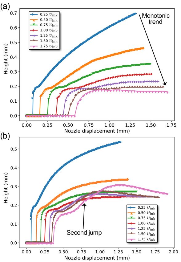
The height of the printed thread in Fig. 3a is also clearly dependent on the parameter υnozzle . In order to study
the dynamic evolution, we probe the maximum height, h, of the fluid thread behind the moving nozzle, investigating
whether a stationary condition is reached along the deposition process.
The thread height, h, as a function of the distance travelled by the moving nozzle is reported in Fig. 3. In both
the case of 1% and 3% concentrations, the height of the thread for lowest nozzle velocities, υnozzle = 0.25 υink does
not show any asymptotic trend, confirming that the printing precision is deteriorated by a low dispensing velocity.
We also observe that the asymptotic values in h decrease as the nozzle velocity increases for the 1% concentration,
highlighting a clear, monotonic trend, which is in agreement with the experimental observations reported by Webb
and Doyle14 . It is worth to highlight as the numerical results trace qualitatively the experimental trend, although the
model has been implemented in the two-dimensional framework, endorsing the validity of the dimension reduction.
The height evolution at high velocity and concentration 3% w/v shows a second jump, namely the thickness obtained
at higher values of υnozzle overcomes the value measured with lower velocities υnozzle = [0.75, 1.00, 1.25] υink , providing
a non monotonic trend. This suggests that, at least at high ink concentration, an optimum operating value exists for
the dispensing velocity, compared to the ink delivery rate, which minimises the thread height. Further, the sequence of
asymptotes is found to be monotonic also in the case of 2% solutions at 25 ◦ C, while the sequence with concentration
3% w/v and 40 ◦ C shows the same non-monotonic trend already observed at 25 ◦ C. The non monotonic hight trends
observed for 3% alginate concentrations (both at 25 ◦ C and 40 ◦ C) is produced by the presence of irregularities in
the thread shapes as the one represented in Fig. 4. These irregularities manifest for large nozzle velocites and 3%
alginate concetrations are explained by viscous effect (see the discussion below) and determine also the behaviour
of the coverage ratio. The coverage ratio, reported for the four cases in Figure 2(b), allows a similar classification,
showing a maximum around υnozzle ≈ 0.8υink for solutions with 3% concentration. Then, the coverage ratio decreases
at higher nozzle velocity values due to the irregular shape of the deposited ink as reported in the ink density map of
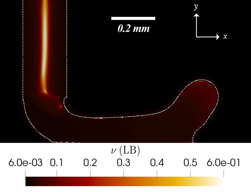
Fig. 2 (panel a). The distinct irregular signature in the thread decreases the coverage ration at υnozzle = 1.75υink .9 Figure 2. (a) Yellow fluid densities for 1% alginate solution. From top to bottom the nozzle velocities υnozzle are equal to 1.75 υink , 1.0 υink , and 0.25 υink . The snapshots are taken as the nozzle has travelled six times, 6d, the nozzle diameter from the lattice position where the ink touches the deposition substrate. In the middle panel, we also sketch thread height (h), the area of the ink thread (Ai ), and the area of the rectangle circumscribing the thread (Ar ) defining the coverage ratio, Ai /Ar .(b) Coverage ratio obtained by different printing parameters. In Fig. 4, the fluid viscosity of the mixture is reported for the case 3% w/v at 25 ◦ C after the ink is deposited. As a first, we observe in Fig. 4 overall a low viscosity in the extruded fluid part which is the result the shear rate enforced among the moving nozzle and the substrate. In all the simulations, we observe a detachment point of the ink from the substrate. In particular, the shearing force produces the detachment point just after the ink reaches the substrate. Later, the detachment point remains visible as an irregular blob in the thread (see Fig. 4). Then, the tread reabsorbs the blob under the action of the capillary pressure. Hence, the rheological behaviour of non-Newtonian inks play a central role in this process. In particular, the relation between shear-rate and the viscosity tunes the magnitude of the transmitted nozzle movements to the deposited ink, biasing both the thread shape and the quality of the final
10

Figure 3. Thread height as a function of the nozzle displacement, for a 1% (a) and a 3% w/v alginate solution. Temperature
= 25 ◦ C

products. Further, it is observed the presence of a low viscosity close to the wall of the nozzle(see Fig. 4), which
is consistent with the Poiseuille flow as a consequence of the larger velocity gradient, ∂υ/∂x, close to the no-slip
boundaries. On the other hand, the viscosity profile shows a high peak in the middle of the nozzle (corresponding to
the lowest velocity gradient point), which can be relevant for the cell viability in bio-inks. Indeed, in the context of
cell culture applications, shear stress is essential to control cell viability, which may be compromised by the impact
force generated by high gradient in viscosity within the nozzle channel52,53 .
   The P OIinorm values, for thread heights less than two times the nozzle diameter, are assessed and shown in Fig 5.
Increasing the alginate concentration results in higher P OIinorm values, which is mainly due to the higher coverage
ratios Ai /Ar alongside with smaller variation in the ink pressure. In particular, for 3% w/v concentrations, the ratio
∆pm /p0 is found in the range from 0.1 to 0.2 for slow nozzle velocity υnozzle < 0.8υink . On the contrary, ∆pm /∆p0 is
always larger than 0.4 for 1% and 2% w/v and for all the nozzle velocities, providing lower P OIinorm values. Thus,
the P OIinorm shows a peak at moderate nozzle speed in the range 0.6-0.8 υink at high alginate concentration 3 %
w/v, due to the simultaneous concourse of high coverage ratios and small ink pressure variations.
   Finally, in some cases, small porosity was noted in the ink fluid (see the upper panel of Fig. 2). In order to address
the question, the POI values were reconsidered, taking into account the porosity. Indeed, since Ai represents the area
11

Figure 4. Kinematic viscosity map of the mixture, ν, for the case 3% w/v at 25 ◦ C, in LB units, after the ink is deposited.
The dashed white line highlights the fluid interface. The ink on the right side features higher viscosity than in the contact line
with the substrate.

Figure 5. Parameter optimization index, reported for thread heights less than two times the nozzle diameter, for different
alginate concentrations and temperatures.

covered by the ink, the area decreases as the porosity increases in the fluid, whenever the porous are excluded in the
Ai assessment. The POI results are practically unaffected by this new definition, with Ai values always changing less
than 1%. Consequently, the porosity in the trend-line does not bias the features of printed material in the present
simulations, and its effect can be reasonably neglected.

V.   CONCLUSIONS

   Summarising, we have introduced a multi-component model of non-Newtonian inks through a regularised version
of the colour gradient LB model and used it to simulate the 2D printing process as a function of a number of design
12

parameters. The model allows to calculate the shear stresses during the printing process of non Newtonian inks,
directly accessible by simulations, that is very important to control the cell viability in bio-inks. The print accuracy
was quantitatively analysed using the same indexes used in experimental studies14 . The impact of the pseudo-plastic
rheology on the printing accuracy was investigated for a set of solutions at different alginate concentration. Systematic
investigations of processes are enabled on a broad viscosity range, providing a useful tool to probe the dynamics of
the forces acting inside and on the ink during additive manufacturing. In real systems, shear thinning fluids are
usually employed in order to favour the throughput of the device (small viscosity at high shear rates) and to obtain a
stable and regular thread at the end of deposition (high viscosity at small shear rates). However the accuracy of the
deposited threads is deteriorated for high viscosity alginate concentration at high print speed since these composites
favour the transmission of the inertia of the fluid impacting the substrate which produce irregularities in the threads.

DATA AVAILABILITY

  Data available on request from the authors.

ACKNOWLEDGMENTS

  The research leading to these results has received funding from MIUR under the project “3D-Phys” (PRIN
2017PHRM8X), and from the European Research Council under the European Union’s Horizon 2020 Framework
Programme (No. FP/2014- 2020)/ERC Grant Agreement No. 739964 ("COPMAT").

REFERENCES

1 R.  L. Truby and J. A. Lewis, Nature 540, 371 (2016).
2 T.  D. Ngo, A. Kashani, G. Imbalzano, K. T. Nguyen, and D. Hui, Composites Part B: Engineering 143, 172 (2018).
 3 R. D. Farahani, M. Dubé, and D. Therriault, Advanced Materials 28, 5794 (2016).
 4 E. Axpe and M. L. Oyen, International journal of molecular sciences 17, 1976 (2016).
 5 B. Utela, D. Storti, R. Anderson, and M. Ganter, Journal of Manufacturing Processes 10, 96 (2008).
 6 M. Lauricella, S. Succi, E. Zussman, D. Pisignano, and A. L. Yarin, Reviews of Modern Physics 92, 035004 (2020).
 7 A. M. Gañán-Calvo, J. M. López-Herrera, M. A. Herrada, A. Ramos, and J. M. Montanero, Journal of Aerosol Science 125, 32 (2018).
 8 S. Succi, The lattice Boltzmann equation: for complex states of flowing matter (Oxford University Press, 2018).
 9 T. Krüger, H. Kusumaatmaja, A. Kuzmin, O. Shardt, G. Silva, and E. M. Viggen, Springer International Publishing 10, 978 (2017).
10 H. Huang, M. Sukop, and X. Lu, Multiphase lattice Boltzmann methods: Theory and application (John Wiley & Sons, 2015).
11 R. Benzi, S. Succi, and M. Vergassola, Physics Reports 222, 145 (1992).
12 M. M. Cross, Journal of colloid science 20, 417 (1965).
13 J. Latt and B. Chopard, Mathematics and Computers in Simulation 72, 165 (2006).
14 B. Webb and B. J. Doyle, Bioprinting 8, 8 (2017).
15 A. Montessori, M. Lauricella, M. La Rocca, S. Succi, E. Stolovicki, R. Ziblat, and D. Weitz, Computers & Fluids 167, 33 (2018).
16 S. Leclaire, A. Parmigiani, O. Malaspinas, B. Chopard, and J. Latt, Physical Review E 95, 033306 (2017).
17 S. Leclaire, M. Reggio, and J.-Y. Trépanier, Journal of Computational Physics 246, 318 (2013).
18 S. Leclaire, A. Parmigiani, B. Chopard, and J. Latt, International Journal of Modern Physics C 28, 1750085 (2017).
19 Z. Wen, Q. Li, Y. Yu, and K. H. Luo, Physical Review E 100, 023301 (2019).
20 S. Saito, Y. Abe, and K. Koyama, Physical Review E 96, 013317 (2017).
21 H. Liu, A. J. Valocchi, and Q. Kang, Physical Review E 85, 046309 (2012).
22 T. Reis and T. Phillips, Journal of Physics A: Mathematical and Theoretical 40, 4033 (2007).
23 M. Latva-Kokko and D. H. Rothman, Physical Review E 72, 046701 (2005).
24 T. Akai, B. Bijeljic, and M. J. Blunt, Advances in water resources 116, 56 (2018).
25 S. Leclaire, K. Abahri, R. Belarbi, and R. Bennacer, International Journal for Numerical Methods in Fluids 82, 451 (2016).
26 R. Zhang, X. Shan, and H. Chen, Physical Review E 74, 046703 (2006).
27 C. G. Coreixas, High-order extension of the recursive regularized lattice Boltzmann method, Ph.D. thesis (2018).
28 A. Montessori, G. Falcucci, P. Prestininzi, M. La Rocca, and S. Succi, Physical Review E 89, 053317 (2014).
29 J. Latt, Hydrodynamic limit of lattice Boltzmann equations, Ph.D. thesis, University of Geneva (2007).
30 M. Lauricella, S. Melchionna, A. Montessori, D. Pisignano, G. Pontrelli, and S. Succi, Physical Review E 97, 033308 (2018).
31 G. Pontrelli, S. Ubertini, and S. Succi, Journal of Statistical Mechanics: Theory and Experiment 2009, P06005 (2009).
32 S. Gabbanelli, G. Drazer, and J. Koplik, Physical review E 72, 046312 (2005).
33 E. Aharonov and D. H. Rothman, Geophysical Research Letters 20, 679 (1993).
34 O. Malaspinas, G. Courbebaisse, and M. Deville, International Journal of Modern Physics C 18, 1939 (2007).
35 R. Ouared and B. Chopard, Journal of statistical physics 121, 209 (2005).
36 B. S. Roopa and S. Bhattacharya, International journal of food science & technology 44, 2583 (2009).
37 A. J. Ladd, Journal of fluid mechanics 271, 285 (1994).
38 F. Jansen and J. Harting, Physical Review E 83, 046707 (2011).
39 A. Ladd and R. Verberg, Journal of statistical physics 104, 1191 (2001).
13 40 C. K. Aidun, Y. Lu, and E.-J. Ding, Journal of Fluid Mechanics 373, 287 (1998). 41 I. Ginzburg, Advances in Water Resources 28, 1196 (2005). 42 A. Kupershtokh, D. Medvedev, and D. Karpov, Computers & Mathematics with Applications 58, 965 (2009). 43 M. Sarker and X. Chen, Journal of Manufacturing Science and Engineering 139 (2017). 44 P. Del Gaudio, P. Colombo, G. Colombo, P. Russo, and F. Sonvico, International journal of pharmaceutics 302, 1 (2005). 45 Y. He, F. Yang, H. M. Zhao, Q. Gao, B. Xia, and J. Z. Fub, Scientific Reports 6, 29977 (2016). 46 J. Ventrici de Souza, Y. Liu, S. Wang, P. Dörig, T. L. Kuhl, J. Frommer, and G.-y. Liu, The Journal of Physical Chemistry B 122, 956 (2018). 47 D. Ye, Y. Ding, Y. Duan, J. Su, Z. Yin, and Y. A. Huang, Small 14, 1703521 (2018). 48 M. Wei, F. Zhang, W. Wang, P. Alexandridis, C. Zhou, and G. Wu, Journal of Power Sources 354, 134 (2017). 49 Y. Jin, W. Chai, and Y. Huang, Materials Science and Engineering: C 80, 313 (2017). 50 Z. Zhang, Y. Jin, J. Yin, C. Xu, R. Xiong, K. Christensen, B. R. Ringeisen, D. B. Chrisey, and Y. Huang, Applied Physics Reviews 5, 041304 (2018). 51 J.-F. Agassant, F. Pigeonneau, L. Sardo, and M. Vincent, Additive Manufacturing 29, 100794 (2019). 52 J. Shi, B. Wu, S. Li, J. Song, B. Song, and W. F. Lu, Biomedical Physics & Engineering Express 4, 045028 (2018). 53 F. Lee, C. Iliescu, F. Yu, and H. Yu, in Methods in cell biology, Vol. 146 (Elsevier, 2018) pp. 43–65.
You can also read


