MAVE-NN: learning genotype-phenotype maps from multiplex assays of variant effect
←
→
Page content transcription
If your browser does not render page correctly, please read the page content below

Tareen et al. Genome Biology     (2022) 23:98
https://doi.org/10.1186/s13059-022-02661-7

 SOFTWARE                                                                                                                                      Open Access

MAVE-NN: learning genotype-phenotype
maps from multiplex assays of variant effect
Ammar Tareen1,2 , Mahdi Kooshkbaghi1 , Anna Posfai1 , William T. Ireland3,4 , David M. McCandlish1 and
Justin B. Kinney1*

*Correspondence:
jkinney@cshl.edu                        Abstract
1
  Simons Center for Quantitative        Multiplex assays of variant effect (MAVEs) are a family of methods that includes deep
Biology, Cold Spring Harbor
Laboratory, Cold Spring Harbor, NY      mutational scanning experiments on proteins and massively parallel reporter assays on
11724, USA                              gene regulatory sequences. Despite their increasing popularity, a general strategy for
Full list of author information is
available at the end of the article
                                        inferring quantitative models of genotype-phenotype maps from MAVE data is lacking.
                                        Here we introduce MAVE-NN, a neural-network-based Python package that imple-
                                        ments a broadly applicable information-theoretic framework for learning genotype-
                                        phenotype maps—including biophysically interpretable models—from MAVE datasets.
                                        We demonstrate MAVE-NN in multiple biological contexts, and highlight the ability of
                                        our approach to deconvolve mutational effects from otherwise confounding experi-
                                        mental nonlinearities and noise.

                                      Background
                                      Over the last decade, the ability to quantitatively study genotype-phenotype (G-P)
                                      maps has been revolutionized by the development of multiplex assays of variant effect
                                      (MAVEs), which can measure molecular phenotypes for thousands to millions of geno-
                                      typic variants in parallel [1, 2]. MAVE is an umbrella term that describes a diverse set
                                      of experimental methods, some examples of which are illustrated in Fig. 1. Deep muta-
                                      tional scanning (DMS) experiments [3] are a type of MAVE commonly used to study
                                      protein sequence-function relationships. These assays work by linking variant proteins
                                      to their coding sequences, either directly or indirectly, then using deep sequencing to
                                      assay which variants survive a process of activity-dependent selection (e.g., Fig. 1a).
                                      Massively parallel reporter assays (MPRAs) are another major class of MAVE and are
                                      commonly used to study DNA or RNA sequences that regulate gene expression at a
                                      variety of steps, including transcription, mRNA splicing, cleavage and polyadenylation,
                                      translation, and mRNA decay [4–7]. MPRAs typically rely on either an RNA-seq readout
                                      of barcode abundances (Fig. 1c) or the sorting of cells expressing a fluorescent reporter
                                      gene (Fig. 1e).

                                      © The Author(s). 2022 Open Access This article is licensed under a Creative Commons Attribution 4.0 International License,
                                      which permits use, sharing, adaptation, distribution and reproduction in any medium or format, as long as you give appropriate
                                      credit to the original author(s) and the source, provide a link to the Creative Commons licence, and indicate if changes were
                                      made. The images or other third party material in this article are included in the article’s Creative Commons licence, unless
                                      indicated otherwise in a credit line to the material. If material is not included in the article’s Creative Commons licence and your
                                      intended use is not permitted by statutory regulation or exceeds the permitted use, you will need to obtain permission directly
                                      from the copyright holder. To view a copy of this licence, visit http://creativecommons.org/licenses/by/4.0/. The Creative
                                      Commons Public Domain Dedication waiver (http://creativecommons.org/publicdomain/zero/1.0/) applies to the data made
                                      available in this article, unless otherwise stated in a credit line to the data.
Tareen et al. Genome Biology      (2022) 23:98                                                                                           Page 2 of 27

                   Fig. 1 Diverse MAVEs and the datasets they produce. a DMS assays using either affinity purification or
                   selective growth. (i) The DMS assay of Olson et al. [8] used a library of variant GB1 proteins physically linked
                   to their coding mRNAs. Functional GB1 proteins were then enriched using IgG beads. (ii) The DMS studies
                   of Seuma et al. [9] and Bolognesi et al. [10] used selective growth in genetically modified Saccharomyces
                   cerevisiae to assay the functionality of variant Aβ and TDP-43 proteins, respectively. In all three experiments,
                   deep sequencing was used to determine an enrichment ratio for each protein variant. b The resulting DMS
                   datasets consist of variant protein sequences and their corresponding log enrichment values. c The MPSA
                   of Wong et al. [11]. A library of 3-exon minigenes was constructed from exons 16, 17, and 18 of the human
                   BRCA2 gene, with each minigene having a variant 5 ss at exon 17 and a random 20 nt barcode in the 3 UTR.
                   This library was transfected into HeLa cells, and deep sequencing of RNA barcodes was used to quantify
                   mRNA isoform abundance. d The resulting MPSA dataset comprises variant 5 ss with (noisy) PSI values. e The
                   sort-seq MPRA of Kinney et al. [12]. A plasmid library was generated in which randomly mutagenized versions
                   of the Escherichia coli lac promoter drove the expression of GFP. Cells carrying these plasmids were sorted
                   using FACS, and the variant promoters in each bin of sorted cells, as well as the initial library, were sequenced.
                   f The resulting dataset comprises a list of variant promoter sequences, as well as a matrix of counts for each
                   variant in each FACS bin. MAVE: multiplex assay of variant effect; DMS: deep mutational scanning; GB1:
                   protein G domain B1; IgG: immunoglobulin G; Aβ: amyloid beta; TDP-43: TAR DNA-binding protein 43; MPSA:
                   massively parallel splicing assay; BRCA2: breast cancer 2; 5 ss: 5 splice site(s); UTR: untranslated region; PSI:
                   percent spliced in; GFP: green fluorescent protein; FACS: fluorescence-activated cell sorting

                    Most computational methods for analyzing MAVE data have focused on accurately
                  quantifying the activity of individual assayed sequences [13–19]. However, MAVE meas-
                  urements like enrichment ratios or cellular fluorescence levels usually cannot be inter-
                  preted as providing direct quantification of biologically meaningful activities, due to the
Tareen et al. Genome Biology   (2022) 23:98                                                                   Page 3 of 27

                  presence of experiment-specific nonlinearities and noise. Moreover, MAVE data is usu-
                  ally incomplete, as one often wishes to understand G-P maps over vastly larger regions
                  of sequence space than can be exhaustively assayed. The explicit quantitative modeling
                  of G-P maps can address both the indirectness and incompleteness of MAVE meas-
                  urements [1, 20]. The goal here is to determine a mathematical function that, given a
                  sequence as input, will return a quantitative value for that sequence’s molecular phe-
                  notype. Such quantitative modeling has been of great interest since the earliest MAVE
                  methods were developed [12, 21, 22], but no general-use software has yet been described
                  for inferring G-P maps of arbitrary functional form from the diverse types of datasets
                  produced by commonly used MAVEs.
                     Here we introduce a unified conceptual framework for the quantitative modeling of
                  MAVE data. This framework is based on the use of latent phenotype models, which
                  assume that each assayed sequence has a well-defined latent phenotype (specified by the
                  G-P map), of which the MAVE experiment provides a noisy indirect readout (described
                  by the measurement process). The quantitative forms of both the G-P map and the
                  measurement process are then inferred from MAVE data simultaneously. We further
                  introduce an information-theoretic approach for separately assessing the performance
                  of the G-P map and the measurement process components of latent phenotype mod-
                  els. This strategy is implemented in an easy-to-use open-source Python package called
                  MAVE-NN, which represents latent phenotype models as neural networks and infers
                  the parameters of these models from MAVE data using a TensorFlow 2 backend [23].
                     In what follows, we expand on this unified MAVE modeling strategy and apply it to
                  a diverse array of DMS and MPRA datasets. Doing so, we find that MAVE-NN pro-
                  vides substantial advantages over other MAVE modeling approaches. In particular, we
                  illustrate how the ability of MAVE-NN to train custom G-P maps can shed light on the
                  biophysical mechanisms of protein function and gene regulation. We also highlight the
                  substantial benefits of including sequence variants with multiple mutations in assayed
                  sequence libraries, as doing so allows MAVE-NN to deconvolve the features of the G-P
                  map from potentially confounding effects of experimental nonlinearities and noise.
                  Indeed, including just a modest number of multiple-mutation variants in a MAVE
                  experiment can be beneficial even when one is primarily interested in the effects of sin-
                  gle mutations.

                  Results
                  Latent phenotype modeling strategy
                  MAVE-NN supports the analysis of MAVE data on DNA, RNA, and protein sequences
                  and can accommodate either continuous or discrete measurement values. Given a set
                  of sequence-measurement pairs, MAVE-NN aims to infer a probabilistic mapping from
                  sequences to measurements. Our primary enabling assumption, which is encoded in
                  the structure of the latent phenotype model (Fig. 2a), is that this mapping occurs in two
                  stages. Each sequence is first mapped to a latent phenotype by a deterministic G-P map.
                  This latent phenotype is then mapped to possible measurement values via a stochas-
                  tic measurement process. During training, the G-P map and measurement process are
                  simultaneously learned by maximizing a regularized form of likelihood.
Tareen et al. Genome Biology       (2022) 23:98                                                                                              Page 4 of 27

                   Fig. 2 MAVE-NN quantitative modeling strategy. a Structure of latent phenotype models. A deterministic G-P
                   map f(x) maps each sequence x to a latent phenotype φ, after which a probabilistic measurement process
                   p(y|φ) generates a corresponding measurement y. b Example of an MPA measurement process inferred
                   from the sort-seq MPRA data of Kinney et al. [12]. MPA measurement processes are used when y values
                   are discrete. c Structure of a GE regression model, which is used when y is continuous. A GE measurement
                   process assumes that the mode of p(y|φ), called the prediction            is given by a nonlinear function g(φ), and
                                                                                         ŷ,
                   the scatter about this mode is described by a noise model p y|ŷ . d Example of a GE measurement process
                   inferred from the DMS data of Olson et al. [8]. Shown are the nonlinearity, the 68% PI, and the 95% PI. e
                   Information-theoretic quantities used to assess model performance. Intrinsic information, Iint , is the mutual
                   information between sequences x and measurements y. Predictive information, Ipre , is the mutual information
                   between measurements y and the latent phenotype values φ assigned by a G-P map. Variational information,
                   Ivar , is a linear transformation of the log likelihood of a full latent phenotype model. The model performance
                   inequality, Iint ≥ Ipre ≥ Ivar , always holds on test data (modulo finite data uncertainties), with Iint =Ipre when the
                   G-P map is correct, and Ipre =Ivar when the measurement process correctly describes the distribution of y
                   conditioned on φ. G-P: genotype-phenotype; MPA: measurement process agnostic; MPRA: massively parallel
                   reporter assay; GE: global epistasis; DMS: deep mutational scanning; PI: prediction interval

                     MAVE-NN includes four types of built-in G-P maps: additive, neighbor, pairwise,
                  and black box. Additive G-P maps assume that each character at each position within a
                  sequence contributes independently to the latent phenotype. Neighbor G-P maps incor-
                  porate interactions between adjacent (i.e., nearest-neighbor) characters in a sequence,
                  while pairwise G-P maps include interactions between all pairs of characters in a
                  sequence regardless of the distance separating the characters in each pair. Black box G-P
                  maps have the form of a densely connected multilayer perceptron, the specific architec-
                  ture of which can be controlled by the user. MAVE-NN also supports custom G-P maps
                  that can be used, e.g., to represent specific biophysical hypotheses about the mecha-
                  nisms of sequence function.
                     To handle both discrete and continuous measurement values, two different strate-
                  gies for modeling measurement processes are provided. Measurement process agnostic
                  (MPA) regression uses techniques from the biophysics literature [12, 20, 24, 25] to ana-
                  lyze MAVE datasets that report discrete measurements. Here the measurement process
                  is represented by an overparameterized neural network that takes the latent phenotype
                  as input and outputs the probability of each possible categorical measurement (Fig. 2b).
                  Global epistasis (GE) regression (Fig. 2c), by contrast, leverages ideas previously
                  developed in the evolution literature for analyzing datasets that contain continuous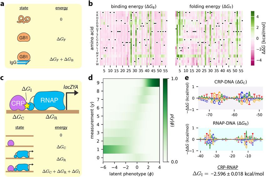
Tareen et al. Genome Biology   (2022) 23:98                                                                      Page 5 of 27

                  measurements [26–29], and is becoming an increasingly popular strategy for modeling
                  DMS data [30–33]. Here, the latent phenotype is nonlinearly mapped to a prediction
                  that represents the most probable measurement value. A noise model is then used to
                  describe the distribution of likely deviations from this prediction. MAVE-NN supports
                  both homoscedastic and heteroscedastic noise models based on three different classes of
                  probability distribution: Gaussian, Cauchy, and skewed-t. In particular, the skewed-t dis-
                  tribution, introduced by Jones and Faddy [34], reduces to Gaussian and Cauchy distribu-
                  tions in certain limits, but also accommodates asymmetric experimental noise. Figure 2d
                  shows an example of a GE measurement process with a heteroscedastic skewed-t noise
                  model.
                     Readers should note that the current implementation of MAVE-NN places constraints
                  on input data and model architecture. Input sequences must be the same length, and
                  when analyzing continuous data, only scalar measurements (as opposed to vectors of
                  multiple measurements) can be used to train models. In addition, because our method
                  for learning the form of experimental nonlinearities depends on observing how multiple
                  mutations combine, MAVE-NN’s functionality is more limited when analyzing MAVE
                  libraries that contain only single-mutation variants. More information on these con-
                  straints and the reasons behind them can be found below in the section “Constraints on
                  datasets and models”.

                  Information-theoretic measures of model performance
                  We further propose three distinct quantities for assessing the performance of latent
                  phenotype models: intrinsic information, predictive information, and variational infor-
                  mation (Fig. 2e). These quantities come from information theory and are motivated by
                  thinking of G-P maps in terms of information compression. In information theory, a
                  quantity called mutual information quantifies the amount of information that the value
                  of one variable communicates about the value of another [35, 36]. Mutual information is
                  symmetric, is nonnegative, and is measured in units called “bits”. If the two variables in
                  question are independent, their mutual information will be zero bits. If instead, know-
                  ing the value of one of these variables allows you to narrow down the value of the other
                  variable to one of two otherwise equally likely possibilities, their mutual information
                  will be 1.0 bits. This mutual information will be 2.0 bits if this second variable’s value
                  is narrowed down to one of four possibilities, 3.0 bits if it is narrowed down to one of
                  eight possibilities, and so on. But importantly, mutual information does not require that
                  the relationship between the two variables of interest be so clean cut, and can in fact
                  be computed between any two types of variables—discrete, continuous, multi-dimen-
                  sional, etc.. This property makes the information-based quantities we propose applicable
                  to all MAVE datasets, regardless of the specific type of experimental readout used. By
                  contrast, many of the standard model performance metrics have restricted domains of
                  applicability: accuracy can only be applied to data with categorical labels, Pearson and
                  Spearman correlation can only be applied to data with univariate continuous labels, and
                  so on. We note, however, that estimating mutual information and related quantities from
                  finite data is nontrivial and that MAVE-NN uses a variety of approaches to do this.
                    Our information metrics are as follows. Intrinsic information, Iint , is the mutual infor-
                  mation between the sequences and measurements contained within a MAVE dataset.
Tareen et al. Genome Biology   (2022) 23:98                                                                     Page 6 of 27

                  This quantity provides a useful benchmark against which to compare the performance
                  of inferred G-P maps. Predictive information, Ipre , is the mutual information between
                  MAVE measurements and the latent phenotype values predicted by an inferred G-P
                  map. This quantifies how well the latent phenotype preserves sequence-encoded infor-
                  mation that is determinative of experimental measurements. When evaluated on test
                  data, Ipre is bounded above by Iint , and equality is realized only when the G-P map loss-
                  lessly compresses sequence-encoded information. Variational information, Ivar , is a
                  linear transformation of log likelihood (or equivalently, cross-entropy) that provides a
                  variational lower bound on Ipre [37–39]. The difference between Ipre and Ivar quantifies
                  how accurately the inferred measurement process matches the observed distribution of
                  measurements conditioned on latent phenotypes (see Additional file 1: Section S1).
                     MAVE-NN infers model parameters by maximizing an (often quite lightly) regularized
                  form of likelihood. These computations are performed using the standard backpropa-
                  gation-based training algorithms provided within TensorFlow 2. With certain caveats
                  noted (see “Methods”), this optimization procedure maximizes Ipre while avoiding the
                  costly estimates of mutual information at each iteration that have hindered the adoption
                  of previous mutual-information-based modeling strategies [12, 25].

                  Application: deep mutational scanning assays
                  We now demonstrate the capabilities of MAVE-NN on three DMS datasets, starting
                  with the study of Olson et al. [8]. These authors measured the effects of single and dou-
                  ble mutations to residues 2–56 of the IgG binding domain of protein G (GB1). To assay
                  the binding of GB1 variants to IgG, the authors combined mRNA display with ultra-
                  high-throughput DNA sequencing [Fig. 1a(i)]. The resulting dataset reports log enrich-
                  ment values for all possible 1045 single mutations and 530,737 (nearly all possible)
                  double-mutations to this 55 aa protein sequence (Fig. 1b).
                    Inspired by the work of Otwinowski et al. [29], we used MAVE-NN to infer a latent
                  phenotype model comprising an additive G-P map and a GE measurement process.
                  This inference procedure required only about 5 min on one node of a computer cluster
                  (Additional file 1: Fig. S1e). Figure 3a illustrates the inferred additive G-P map via the
                  effects that every possible single-residue mutation has on the latent phenotype. From
                  this heatmap of additive effects, we can immediately identify all of the critical GB1 resi-
                  dues, including the IgG-interacting residues at 27, 31, and 43 [8]. We also observe that
                  missense mutations to proline throughout the GB1 domain tend to negatively impact
                  IgG binding, as expected due to this amino acid’s exceptional conformational rigidity.
                    Figure 3b illustrates the corresponding GE measurement process, revealing a sigmoi-
                  dal relationship between log enrichment measurements and the latent phenotype values
                  predicted by the G-P map. Nonlinearities like this are ubiquitous in DMS data due to the
                  presence of background and saturation effects. Unless they are explicitly accounted for
                  in one’s quantitative modeling efforts, as they are here, these nonlinearities can greatly
                  distort the parameters of inferred G-P maps. Figure 3c shows that accounting for this
                  nonlinearity yields predictions that correlate quite well with measurement values.
                    One particularly useful feature of MAVE-NN is that every inferred model can be
                  used as a MAVE dataset simulator (see “Methods”). Among other things, this capabil-
                  ity allows users to verify whether MAVE-NN can recover ground-truth models from
Tareen et al. Genome Biology (2022) 23:98 Page 7 of 27
Fig. 3 Analysis of DMS data for protein GB1. MAVE-NN was used to infer a latent phenotype model,
consisting of an additive G-P map and a GE measurement process with a heteroscedastic skewed-t noise
model, from the DMS data of Olson et al. [8]. All 530,737 pairwise variants reported for positions 2 to 56 of
the GB1 domain were analyzed. Data were split 90:5:5 into training, validation, and test sets. a The inferred
additive G-P map parameters. Gray dots indicate wildtype residues. Amino acids are ordered as in Olson
et al. [8]. b GE plot showing measurements versus predicted latent phenotype values for 5000 randomly
selected test-set sequences (blue dots), alongside the inferred nonlinearity (solid orange line) and the 95%
PI (dotted orange lines) of the noise model. Gray line indicates the latent phenotype value of the wildtype
sequence. c Measurements plotted against ŷ predictions for these same sequences. Dotted lines indicate the
95% PI of the noise model. Gray line indicates the wildtype value of ŷ. Uncertainty in the value of R2 reflects
standard error. d Corresponding information metrics computed during model training (using training data)
or for the final model (using test data). The uncertainties in these estimates are very small—roughly the
width of the plotted lines. Gray shaded area indicates allowed values for intrinsic information based on the
upper and lower bounds estimated as described in “Methods.” e–g Test set predictions (blue dots) and GE
nonlinearities (orange lines) for models trained using subsets of the GB1 data containing all single mutants
and 50,000 (e), 5000 (f), or 500 (g) double mutants. The GE nonlinearity from panel b is shown for reference
(yellow-green lines). DMS: deep mutational scanning; GB1: protein G domain B1; GE: global epistasis; G-P:
genotype-phenotype; PI: prediction interval
realistic datasets in diverse biological contexts. By analyzing simulated data generated
by the model we inferred for GB1, we observed that MAVE-NN could indeed accu-
rately and robustly recover both the GE nonlinearity and the ground-truth G-P map
parameters (Additional file 1: Fig. S1a-d).Tareen et al. Genome Biology (2022) 23:98 Page 8 of 27
Figure 3d summarizes the values of our information-theoretic metrics for model
performance. On held-out test data we find that Ivar =2.178±0.027 bits and
Ipre = 2.225 ± 0.017 bits, where the uncertainties in these values reflect standard errors.
The similarity of these two values suggests that the inferred GE measurement process,
which includes a heteroscedastic skewed-t noise model, very well describes the distri-
bution of residuals. We further find that 2.741 ± 0.013 bits≤Iint ≤3.215 ± 0.007 bits
(see “Methods”), meaning that the inferred G-P map accounts for 69–81% of the total
sequence-dependent information in the dataset. While this performance is impressive,
the additive G-P map evidently misses some relevant aspect of the true genetic architec-
ture. This observation motivates the more complex biophysical model for GB1 discussed
later in “Results”.
The ability of MAVE-NN to deconvolve experimental nonlinearities from additive G-P
maps requires that some of the assayed sequences contain multiple mutations. This is
because such nonlinearities are inferred by reconciling the effects of single mutations
with the effects observed for combinations of two or more mutations. To investigate how
many multiple-mutation variants are required, we performed GE inference on subsets of
the GB1 dataset containing all 1045 single-mutation sequences and either 50,000, 5000,
or 500 double-mutation sequences (see “Methods”). The shapes of the resulting GE
nonlinearities are illustrated in Fig. 3e–g. Remarkably, MAVE-NN is able to recover the
underlying nonlinearity using only about 500 randomly selected double mutants, which
represent only ~0.1% of all possible double mutants. The analysis of simulated data also
supports the ability to accurately recover ground-truth model predictions using highly
reduced datasets (Additional file 1: Fig. S1f). These findings have important implications
for the design of DMS experiments: even if one only wants to determine an additive G-P
map, including a modest number of multiple-mutation sequences in the assayed library
is often advisable because it an enable the removal of artifactual nonlinearities.
To test the capabilities of MAVE-NN on less complete DMS datasets, we analyzed
recent experiments on amyloid beta (Aβ) [9] and TDP-43 [10], both of which exhibit
aggregation behavior in the context of neurodegenerative diseases. In these experiments,
protein functionality was assayed using selective growth [Fig. 1a(ii)] in genetically modi-
fied Saccaromyces cerevisiae: Seuma et al. [9] positively selected for Aβ aggregation,
whereas Bolognesi et al. [10] selected against TDP-43 toxicity. Like with GB1, the variant
libraries used in these two experiments included a substantial number of multiple-muta-
tion sequences: 499 single- and 15,567 double-mutation sequences for Aβ; 1266 single-
and 56,730 double-mutation sequences for TDP-43. But unlike with GB1, these datasets
are highly incomplete due to the use of mutagenic PCR (for Aβ) or doped oligo synthesis
(for TDP-43) in the construction of variant libraries.
We used MAVE-NN to infer additive G-P maps from these two datasets, adopting the
same type of latent phenotype model used for GB1. Figure 4a illustrates the additive G-P
map inferred from aggregation measurements of Aβ variants. In agreement with the
original study, we see that most amino acid mutations between positions 30–40 have
a negative effect on variant enrichment, suggesting that this region plays a major role
in promoting nucleation. Figure 4b shows the corresponding measurement process (see
also Additional file 1: Fig. S2). Even though these data are much sparser than the GB1
data, the inferred model performs well on held-out test data (Ivar = 1.142 ± 0.065 bits,Tareen et al. Genome Biology (2022) 23:98 Page 9 of 27
Fig. 4 Analysis of DMS data for Aβ and TDP-43. a, b Seuma et al. [9] measured nucleation scores for 499
single mutants and 15,567 double mutants of Aβ. These data were used to train a latent phenotype model
comprising a an additive G-P map and b a GE measurement process with a heteroscedastic skewed-t noise
model. c, d Bolognesi et al. [10] measured toxicity scores for 1266 single mutants and 56,730 double mutants
of TDP-43. The resulting data were used to train c an additive G-P map and d a GE measurement process of
the same form as in panel b. In both cases, data were split 90:5:5 into training, validation, and test sets. In a,
c, gray dots indicate the wildtype sequence and * indicates a stop codon. White squares [355/882 (40.2%) for
Aβ; 433/1764 (24.5%) for TDP-43] indicate residues that were not observed in the training set and thus could
not be assigned values for their additive effects. Amino acids are ordered as in the original publications [9,
10]. In b, d, blue dots indicate latent phenotype values plotted against measurements for held-out test data.
Gray line indicates the latent phenotype value of the wildtype sequence. Solid orange line indicates the GE
nonlinearity, and dotted orange lines indicate a corresponding 95% PI for the inferred noise model. Values for
Ivar , Ipre , and R2 (between y and ŷ) are also shown. Uncertainties reflect standard errors. Additional file 1: Fig.
S2 shows measurements plotted against the ŷ predictions of these models. DMS: deep mutational scanning;
Aβ: amyloid beta; TDP-43: TAR DNA-binding protein 43; G-P: genotype-phenotype; GE: global epistasis; PI:
prediction interval
Ipre = 1.187± 0.050 bits, R2 = 0.763 ± 0.024). Similarly, Fig. 4c, d show the G-P map
parameters and GE measurement process inferred from toxicity measurements of TDP-
43 variants, revealing among other things the toxicity-determining hot-spot observed by
Bolognesi et al. [10] at positions 310–340. Again, the resulting latent phenotype model
performs well on held-out test data (Ivar = 1.834 ± 0.035 bits, I pre =1.994 ± 0.023 bits,
R2 =0.914±0.007).
Application: a massively parallel splicing assay
Exon/intron boundaries are defined by 5 splice sites (5 ss), which bind the U1 snRNP
during the initial stages of spliceosome assembly. To investigate how 5 ss sequence quan-
titatively controls alternative mRNA splicing, Wong et al. [11] used a massively parallel
splicing assay (MPSA) to measure percent spliced in (PSI) values for nearly all 32,768
possible 5 ss of the form NNN/GYNNNN in three different genetic contexts (Fig. 1c,d).
Applying MAVE-NN to data from the BRCA2 exon 17 context, we inferred four differ-
ent types of G-P maps: additive, neighbor, pairwise, and black box. As with GB1, these
G-P maps were each inferred using GE regression with a heteroscedastic skewed-t noiseTareen et al. Genome Biology (2022) 23:98 Page 10 of 27
model. For comparison, we also inferred an additive G-P map using the epistasis pack-
age of Sailer and Harms [28].
Figure 5a compares the performance of these G-P map models on held-out test data,
while Fig. 5b–d illustrate the corresponding inferred measurement processes. We
observe that the additive G-P map inferred using the epistasis package [28] exhibits less
predictive information (Ipre =0.180 ± 0.011 bits) than the additive G-P map found using
MAVE-NN (P = 3.8×10⁻⁶ , two-sided Z-test). This is likely because the epistasis pack-
age estimates the parameters of the additive G-P map prior to estimating the GE non-
linearity. We also note that, while the epistasis package provides a variety of options for
modeling the GE nonlinearity, none of these options appear to work as well as our more
flexible sum-of-sigmoids approach (compare Fig. 5b,c). This finding again demonstrates
that the accurate inference of G-P maps requires the explicit and simultaneous modeling
of experimental nonlinearities.
We also observe that increasingly complex G-P maps exhibit increased accuracy.
For example, the additive G-P map gives Ipre = 0.257 ± 0.013 bits, whereas the pairwise
G-P map (Fig. 5d, f) attains Ipre = 0.374 ± 0.014 bits. Using MAVE-NN’s built-in para-
metric bootstrap approach for quantifying parameter uncertainty, we find that both
the additive and pairwise G-P map parameters are very precisely determined (see
Additional file 1: Fig. S3). The black box G-P map, which is comprised of 5 densely
connected hidden layers of 10 nodes each, performed the best of all four G-P maps,
achieving Ipre = 0.458 ± 0.015 bits. Remarkably, this predictive information reaches
the lower bound on the intrinsic information estimated from replicate experiments
(Iint ≥ 0.462±0.009 bits; see “Methods”). The black box G-P map can, therefore, explain
all of the apparent sequence-dependence in this MPSA dataset. We thus conclude
that pairwise interaction models are not flexible enough to fully account for how 5 ss
sequences control splicing. More generally, these results underscore the need for soft-
ware that is capable of inferring and assessing a variety of different G-P maps through a
uniform interface.
Application: biophysically interpretable G-P maps
Biophysical models, unlike the phenomenological models considered thus far, have
mathematical structures that reflect specific hypotheses about how sequence-depend-
ent interactions between macromolecules mechanistically define G-P maps. Thermody-
namic models, which rely on a quasi-equilibrium assumption, are the most commonly
used type of biophysical model [41–43]. Previous studies have shown that precise ther-
modynamic models can be inferred from MAVE datasets [12, 44–46], but no software
intended for use by the broader MAVE community has yet been developed for doing
this. MAVE-NN meets this need by enabling the inference of custom G-P maps. We
now demonstrate this biophysical modeling capability in the contexts of protein-ligand
binding [using the DMS data of Olson et al. [8]; Fig. 1a(i)] and bacterial transcriptional
regulation (using sort-seq MPRA data from Kinney et al. [12]; Fig. 1e). An expanded
discussion of how these models are mathematically formulated and specified within
MAVE-NN is provided in Additional file 1: Section S3.
Otwinowski [47] showed that a three-state thermodynamic G-P map (Fig. 6a), one
that accounts for GB1 folding energy in addition to GB1-IgG binding energy, [48] canTareen et al. Genome Biology (2022) 23:98 Page 11 of 27
Fig. 5 Analysis of MPSA data from Wong et al. [11]. This dataset reports PSI values, measured in the BRCA2
exon 17 context, for nearly all 32,768 variant 5 ss of the form NNN/GYNNNN. Data were split 60:20:20 into
training, validation, and test sets. Latent phenotype models were inferred, each comprising one of four types
of G-P map (additive, neighbor, pairwise, or black box), together with a GE measurement process having
a heteroscedastic skewed-t noise model. The epistasis package of Sailer and Harms [28] was also used to
infer an additive G-P map and GE nonlinearity. a Performance of trained models as quantified by Ivar and
Ipre , both computed on test data. The lower bound on Iint was estimated from experimental replicates (see
“Methods”). The p-value reflects a two-sided Z-test. Ivar was not computed for the additive (epistasis package)
model because that package does not infer an explicit noise model. b–d Measurement values versus latent
phenotype values, computed on test data, using the additive (epistasis package) model (b), the additive
model (c), and the pairwise model (d). The corresponding GE measurement processes are also shown. e
Sequence logo [40] illustrating the additive component of the pairwise G-P map. Dashed line indicates the
exon/intron boundary. The G at +1 serves as a placeholder because no other bases were assayed at this
position. At position +2, only U and C were assayed. f Heatmap showing the pairwise component of the
pairwise G-P map. White diagonals correspond to unobserved bases. Additional file 1: Fig. S3 shows the
uncertainties in the values of parameters that are illustrated in panels e and f. Error bars indicate standard
errors. MPSA: massively parallel splicing assay; PSI: percent spliced in; G-P: genotype-phenotype; GE: global
epistasis
explain the DMS data of Olson et al. [8] better than a simple additive G-P map does.
This biophysical model subsequently received impressive confirmation in the work
of Nisthal et al. [49], who measured the thermostability of 812 single-mutation GB1Tareen et al. Genome Biology (2022) 23:98 Page 12 of 27
Fig. 6 Biophysical models inferred from DMS and MPRA data. a Thermodynamic model for IgG binding
by GB1. This model assumes that GB1 can be in one of three states (unfolded, folded-unbound, and
folded-bound). The Gibbs free energies of folding (GF ) and binding (GB ) are computed from sequence
using additive models, which in biophysical contexts like these are called energy matrices [1, 12]. The
latent phenotype is given by the fraction of time GB1 is in the folded-bound state. b The G parameters
of the energy matrices for folding and binding, inferred from the data of Olson et al. [8] by fitting this
thermodynamic model using GE regression. The amino acid ordering used here matches that of Otwinowski
[47]. Additional file 1: Fig. S5 plots folding energy predictions against the measurements of Nisthal et al.
[49]. c A four-state thermodynamic model for transcriptional activation at the E. coli lac promoter. The
Gibbs free energies of RNAP-DNA binding (GR ) and CRP-DNA binding (GC ) are computed using energy
matrices, whereas the CRP-RNAP interaction energy GI is a scalar. The latent phenotype is the fraction of
time a promoter is bound by RNAP. d,e The latent phenotype model inferred from the sort-seq MPRA data
of Kinney et al. [12]. This model includes both the MPA measurement process (d) and the parameters of the
thermodynamic G-P map (e). Additional file 1: Fig. S4 provides detailed definitions of the thermodynamic
models in panels a and c. Sequence logos in panel e were generated using Logomaker [40]. Standard errors
on GI were determined using the parametric bootstrap approach described in “Methods”. DMS: deep
mutational scanning; MPRA: massively parallel reporter assay; IgG: immunoglobulin G; GB1: protein G domain
B1; GE: global epistasis. RNAP: σ70 RNA polymerase; CRP: cAMP receptor protein; MPA: measurement-process
agnostic. G-P: genotype-phenotype
variants. We tested the ability of MAVE-NN to recover the same type of thermodynamic
model that Otwinowski had inferred using custom analysis scripts. MAVE-NN yielded
a G-P map with significantly improved performance on the data of Olson et al. [8]
(Ivar=2.303±0.013 bits, Ipre = 2.357± 0.007 bits, R2 = 0.947± 0.001) relative to the addi-
tive G-P map of Fig. 3a-d. Figure 6b shows the two inferred energy matrices that respec-
tively describe the effects of every possible single-residue mutation on the Gibbs free
energies of protein folding and protein-ligand binding. The folding energy predictions
of our model also correlate as well with the data of Nisthal et al. [49] (R2 = 0.570±0.049)
as the predictions of Otwinowski’s model do (R2 = 0.515 ± 0.056). This demonstrates
that MAVE-NN can infer accurate and interpretable quantitative models of protein
biophysics.Tareen et al. Genome Biology (2022) 23:98 Page 13 of 27
To test MAVE-NN’s ability to infer thermodynamic models of transcriptional regu-
lation, we re-analyzed the MPRA data of Kinney et al. [12], in which random muta-
tions to a 75-bp region of the Escherichia coli lac promoter were assayed (Fig. 1e). This
promoter region binds two regulatory proteins, σ70 RNA polymerase (RNAP) and the
transcription factor CRP. As in Kinney et al. [12], we proposed a four-state thermody-
namic model that quantitatively explains how promoter sequences control transcription
rate (Fig. 6c). The parameters of this G-P map include the Gibbs free energy of interac-
tion between CRP and RNAP (GI ), as well as energy matrices that describe the CRP-
DNA and RNAP-DNA interaction energies (GC and GR , respectively). Because the
sort-seq MPRA of Kinney et al. [12] yielded discrete measurements (Fig. 1f), we used
an MPA measurement process in our latent phenotype model (Fig. 6d). The biophysical
parameters we thus inferred (Fig. 6e), which include a CRP-RNAP interaction energy of
GI = −2.598 ± 0.018 kcal/mol, largely match those of Kinney et al., but were obtained
far more rapidly (in ∼10 min versus multiple days) thanks to the use of stochastic gradi-
ent descent rather than Metropolis Monte Carlo.
Constraints on datasets and models
As mentioned above, MAVE-NN places certain limitations on both input datasets and
latent phenotype models. Some of these constraints have been adopted to simplify the
initial release of MAVE-NN and can be relaxed in future updates. Others reflect fun-
damental mathematical properties of latent phenotype models. Here we summarize the
primary constraints users should be aware of.
MAVE-NN currently requires that all input sequences be the same length. This con-
straint has been adopted because a large fraction of MAVE datasets have this form, and
all of the built-in G-P maps operate only on fixed-length sequences. Users who wish to
analyze variable length sequences can still do so by padding the ends of sequences with
dummy characters. Alternatively, users can provide a multiple-sequence alignment as
input and include the gap character as one of the characters to consider when training
models.
As previously stated, MAVE-NN can analyze MAVE datasets that have either continu-
ous or discrete measurements. At present, both types of measurements must be one-
dimensional, i.e., users cannot fit a single model to vectors of multiple measurements
(e.g., joint measurements of protein binding affinity and protein stability, as in Faure
et al. [31]). This constraint has been adopted only to simplify the user interface of the ini-
tial release. It is not a fundamental limitation of latent phenotype models and is sched-
uled to be relaxed in upcoming versions of MAVE-NN.
The current implementation of MAVE-NN also supports only one-dimensional latent
phenotypes (though the latent phenotype of custom G-P maps can depend on multiple
precursor phenotypes, e.g., binding energy or folding energy). This restriction was made
because accurately interpreting multi-dimensional latent phenotypes is substantially
more fraught than interpreting one-dimensional latent phenotypes, and we believe that
additional computational tools need to be developed to facilitate such interpretation.
That being said, the mathematical form of latent phenotype models is fully compatible
with multi-dimensional latent phenotypes. Indeed, this modeling strategy has been usedTareen et al. Genome Biology (2022) 23:98 Page 14 of 27
in other work [24, 31–33], and we plan to enable this functionality in future updates to
MAVE-NN.
More fundamental constraints come into play when analyzing MAVE data that con-
tains only single-mutation variants. In such experiments, the underlying effects of
individual mutations are hopelessly confounded by the biophysical, physiological, and
experimental nonlinearities that may be present. By contrast, when the same mutation
is observed in multiple genetic backgrounds, MAVE-NN can use systematic differences
in the mutational effects observed between stronger and weaker backgrounds to remove
these confounding influences. Thus, for datasets that probe only single-mutant effects,
we limit MAVE-NN to inferring only additive G-P maps using GE regression, and while
the noise model in the GE measurement process is allowed to be heteroscedastic, the
nonlinearity is constrained to be linear.
We emphasize that, in practice, only a modest number of multiple-mutation variants
are required for MAVE-NN to learn the form of a nonlinear measurement process (see
Fig. 3e–g). In this way, including a small fraction of the possible double-mutation vari-
ants in MAVE libraries can be beneficial even just for determining the effects of single
mutations. Adding such non-comprehensive sets of double mutants to MAVE libraries
is experimentally straight-forward, and our numerical experiments suggest that assay-
ing roughly the same number of double-mutation variants as single-mutation variants
should often suffice. We therefore recommend that experimentalists—even those pri-
marily interested in the effects of single mutations—consider augmenting their MAVE
libraries with a small subset of double-mutation variants.
Discussion
We have presented a unified strategy for inferring quantitative models of G-P maps from
diverse MAVE datasets. At the core of our approach is the conceptualization of G-P
maps as a form of information compression, i.e., the G-P map first compresses an input
sequence into a latent phenotype value, which is then read out indirectly via a noisy and
nonlinear measurement process. By explicitly modeling this measurement process, one
can remove potentially confounding effects from the G-P map, as well as accommodate
diverse experimental designs. We have also introduced three information-theoretic met-
rics for assessing the performance of the resulting models. These capabilities have been
implemented within an easy-to-use Python package called MAVE-NN.
We have demonstrated the capabilities of MAVE-NN in diverse biological contexts,
including in the analysis of both DMS and MPRA data. We have also demonstrated
the superior performance of MAVE-NN relative to the epistasis package of Sailer and
Harms [28]. Along the way, we observed that MAVE-NN can deconvolve experimental
nonlinearities from additive G-P maps when a relatively small number of sequences con-
taining multiple mutations are assayed. This capability provides a compelling reason for
experimentalists to include such sequences in their MAVE libraries, even if they are pri-
marily interested in the effects of single mutations. Finally, we showed how MAVE-NN
can learn biophysically interpretable G-P maps from both DMS and MPRA data.
MAVE-NN thus fills a critical need in the MAVE community, providing user-friendly
software capable of learning quantitative models of G-P maps from diverse MAVE data-
sets. MAVE-NN has a streamlined user interface and is readily installed from PyPI byTareen et al. Genome Biology (2022) 23:98 Page 15 of 27
executing “pip install mavenn” at the command line. Comprehensive documentation and
step-by-step tutorials are available at http://mavenn.readthedocs.io [50].
Methods
Notation
N−1
We represent each MAVE dataset as a set of N observations, (xn , yn ) n=0 , where each
observation consists of a sequence xn and a measurement yn . Here, yn can be either a
continuous real-valued number, or a nonnegative integer representing a “bin” in which
the nth sequence was found. Note that, in this representation, the same sequence x can
be observed multiple times, potentially with different values for y due to experimental noise.
G-P maps
We assume that all sequences have the same length L, and that at each of the L positions
in each sequence there is one of C possible characters. MAVE-NN represents sequences
using a vector of one-hot encoded features of the form
1 if character c occurs at position l
xl:c = , (1)
0 otherwise
where l = 0, 1, . . . , L − 1 indexes positions within the sequence, and c indexes the C dis-
tinct characters in the alphabet. MAVE-NN supplies built-in alphabets for DNA, RNA
and protein (with or without stop codons), and supports custom alphabets as well.
We assume that the latent phenotype is given by a linear function φ(x; θ) that depends
on a set of G-P map parameters θ. As mentioned in the main text, MAVE-NN supports
four types of G-P map models, all of which can be inferred using either GE regression or
MPA regression. The additive model is given by
L−1
φadditive (x; θ) = θ0 + θl:c xl:c . (2)
l=0 c
Here, each position in x contributes independently to the latent phenotype. The neigh-
bor model is given by
L−1
L−2
φneighbor (x; θ) = θ0 + θl:c xl:c + θl:c,(l+1):c xl:c x(l+1):c , (3)
l=0 c l=0 c,c
and further accounts for potential epistatic interactions between neighboring positions.
The pairwise model is given by
L−1
L−2
L−1
φpairwise (x; θ) = θ0 + θl:c xl:c + θl:c,l :c xl:c xl :c , (4)
l=0 c l=0 l =l+1 c,c
and includes interactions between all pairs of positions. Note our convention of requir-
ing l > l in the pairwise parameters θl:c,l :c .
Unlike these three parametric models, the black box G-P map does not have a fixed
functional form. Rather, it is given by a multilayer perceptron that takes a vector of
sequence features (additive, neighbor, or pairwise) as input, contains multiple fullyTareen et al. Genome Biology (2022) 23:98 Page 16 of 27
connected hidden layers with nonlinear activations, and has a single node output with
a linear activation. Users are able to specify the number of hidden layers, the number of
nodes in each hidden layer, and the activation function used by these nodes.
MAVE-NN further supports custom G-P maps, which users can define by subclass-
ing the G-P map base class. These G-P maps can have arbitrary functional forms, e.g.,
representing specific biophysical hypotheses. This feature of MAVE-NN is showcased in
Fig. 6.
Gauge modes and diffeomorphic modes
G-P maps typically have non-identifiable degrees of freedom that must be fixed, i.e.,
pinned down, before the values of individual parameters can be meaningfully inter-
preted or compared between models. These degrees of freedom come in two flavors:
gauge modes and diffeomorphic modes. Gauge modes are changes to θ that do not alter
the values of the latent phenotype φ. Diffeomorphic modes [20, 24] are changes to θ that
do alter φ, but do so in ways that can be undone by transformations of the measurement
process p(y|φ). As shown by Kinney and Atwal [20, 24], the diffeomorphic modes of
linear G-P maps (such as the additive and pairwise G-P maps featured in Figs. 3, 4, and
5) will typically correspond to affine transformations of φ, although additional uncon-
strained modes can occur in special situations.
MAVE-NN automatically fixes the gauge modes and diffeomorphic modes of inferred
models (except when using custom G-P maps). The diffeomorphic modes of G-P maps
are fixed by transforming θ via
θ0 → θ0 − a, (5)
and then
θ
θ→ , (6)
b
where a=mean({φn }) and b=std({φn }) are the mean and standard deviation of φ values
computed on the training data. This produces a corresponding change in latent pheno-
type values φ → (φ − a)/b. To avoid altering model likelihood, MAVE-NN makes a cor-
responding transformation to the measurement process p(y|φ). In GE regression this is
done by adjusting the GE nonlinearity via
g (φ) → g a + bφ , (7)
while keeping the noise model p y|ŷ fixed. In MPA regression, MAVE-NN transforms
the full measurement process via
p y|φ → p y|a + bφ . (8)
For the three parametric G-P maps, gauge modes are fixed using what we call the
“hierarchical gauge”. Here, the parameters θ are adjusted so that the lower-order terms in
φ(x; θ) account for the highest possible fraction of variance in φ. This procedure requires
a probability distribution on sequence space with respect to which these variances are
computed. MAVE-NN assumes that such distributions factorize by position and canTareen et al. Genome Biology (2022) 23:98 Page 17 of 27
thus be represented by a probability matrix with elements pl:c , denoting the probability
of character c at position l. MAVE-NN provides three built-in choices for this distribu-
tion: uniform, empirical, or wildtype. The corresponding values of pl:c are given by
⎧
⎪
⎨ 1/C for uniform
pl:c = nl:c /N for empirical , (9)
⎪
⎩ WT
xl:c for wildtype
where nl:c denotes the number of observations in the dataset (out of N total) for which
the sequence has character c at position l, and xWT
l:c is the one-hot encoding of a user-
specified wildtype sequence. In particular, the wildtype gauge is used for illustrating the
additive G-P maps in Figs. 3 and 4, while the uniform gauge is used for illustrating the
pairwise G-P map in Fig. 5 and the energy matrices in Fig. 6. After a sequence distribu-
tion is chosen, MAVE-NN fixes the gauge of the pairwise G-P map by transforming
θ0 → θ0
+ θl:c pl:c
l c (10)
+ θl:c,l :c pl:c pl :c ,
l l >l c,c
θl:c → θl:c
− θl:c pl:c
c
+ θl:c,l :c pl :c
l >l c
+ θl :c ,l:c pl :c (11)
l l c ,c
− θl:c ,l :c pl:c pl :c ,
lTareen et al. Genome Biology (2022) 23:98 Page 18 of 27
GE nonlinearities
GE models assume that each measurement y is a nonlinear function g (·) of the latent
phenotype φ, plus some noise. In MAVE-NN, this nonlinearity is represented as a sum
of hyperbolic tangent sigmoids:
K−1
g (φ; α) = a + bk tanh (ck φ + dk ) . (13)
k=0
Here, K specifies the number of hidden nodes contributing to the sum, and
α = {a, bk , ck , dk } are trainable parameters. We note that this mathematical form is an
example of the bottleneck architecture previously used by others [27, 33] for modeling
GE nonlinearities. By default, MAVE-NN constrains g(φ; α) to be monotonic in φ by
requiring all bk ≥0 and ck ≥0, but this constraint can be relaxed.
GE noise models
MAVE-NN supports three types of GE noise model: Gaussian, Cauchy, and skewed-t.
All of these noise models support the analytic computation of quantiles and prediction
intervals, as well as the rapid sampling of simulated measurement values. The Gaussian
noise model is given by
2
1 y − ŷ
pgauss y|ŷ; s = √ exp − , (14)
2πs2 2s2
where s denotes the standard deviation. Importantly, MAVE-NN allows this noise model
to be heteroscedastic by representing s as an exponentiated polynomial in ŷ, i.e.,
K
s ŷ = exp ak ŷk , (15)
k=0
where K is the order of the polynomial and {ak } are trainable parameters. The user has
the option to set K, and setting K = 0 renders this noise model homoscedastic. Quantiles
√
are computed using yq = ŷ + s 2 erf−1 (2q − 1) for user-specified values of q ∈[ 0, 1].
Similarly, the Cauchy noise model is given by
2 −1
y − ŷ
pcauchy y|ŷ; s = πs 1 + , (16)
s2
where the scale parameter s is an exponentiated K-order polynomial in ŷ, and quantiles
are computed using yq = ŷ + s tan π q − 12 .
The skewed-t noise model is of the form described by Jones and Faddy [34] and is
given by
pskewt y|ŷ; s, a, b = s−1 f (t; a, b) , (17)Tareen et al. Genome Biology (2022) 23:98 Page 19 of 27
where
√
y − ŷ ∗
∗ (a − b) a + b
t=t + , t = √ √ , (18)
s 2a + 1 2b + 1
and
a+ 1 b+ 1
21−a−b (a + b) t 2 t 2
f (t; a, b) = √ 1+ √ × 1− √ .
a + b (a) (b) a+b+t 2 a+b+t 2
(19)
Note that the t statistic here is an affine function of y chosen so that the distribution’s
mode (corresponding to t ∗ ) is positioned at ŷ. The three parameters of this noise model,
{s, a, b}, are each represented using K-order exponentiated polynomials with trainable
coefficients. Quantiles are computed using
yq = ŷ + tq − t ∗ s, (20)
where
√
2xq − 1 a + b −1
tq = 2 , xq = Iq (a, b) , (21)
1 − 2xq − 1
and Iq−1 (a, b) denotes the inverse of the regularized incomplete Beta function Ix (a, b).
Empirical noise models
MAVE-NN further supports the inference of GE regression models that account for
user-specified measurement noise. In such cases, the user provides a set of measure-
ment-specific standard errors, {sn }N−1
n=0 , along with the corresponding observations.
These uncertainties can, for example, be estimated by using a software package like
Enrich2 [16] or DiMSum [19]. MAVE-NN then trains the parameters of latent pheno-
type models by assuming a Gaussian noise model of the form
2
1 yn − ŷn
pempirical yn |ŷn , sn = exp − , (22)
2πs2n 2s2n
where ŷn = g f (xn ; θ) ; α is the expected measurement for sequence xn , θ denotes G-P
map parameters, and α denotes the parameters of the GE nonlinearity. This noise model
thus has the advantage of having no free parameters, but it may be problematically mis-
specified if the true error distribution is heavy-tailed or skewed.
MPA measurement process
In MPA regression, MAVE-NN directly models the measurement process p(y|φ). At
present, MAVE-NN only supports MPA regression for discrete values of y, which
must be indexed using nonnegative integers. MAVE-NN supports two alternative
forms of input for MPA regression. One is a set of sequence-measurement pairs,
N−1
(xn , yn ) n=0 , where N is the total number of reads, {xn } is a set of (typically non-
unique) sequences, each yn ∈ {0, 1, . . . , Y −1} is a bin number, and Y is the total numberTareen et al. Genome Biology (2022) 23:98 Page 20 of 27
of bins. The other is a set of sequence-count-vector pairs, {(xm , cm )}M−1m=0 , where M is
the total number of unique sequences and cm = (cm0 , cm1 , . . . , cm(Y −1) ) is a vector that
lists the number of times cmy that the sequence xm was observed in each bin y. MPA
measurement processes are represented as a multilayer perceptron with one hidden
layer (having tanh activations) and a softmax output layer. Specifically,
wy (φ)
p y|φ = , (23)
y wy (φ)
where
K−1
wy φ = exp ay + byk tanh cyk φ + dyk , (24)
k=0
and K is the number of hidden nodes per value of y. The trainable parameters of this
measurement process are η = {ay , byk , cyk , dyk }.
Loss function
Let θ denote the G-P map parameters, and η denote the parameters of the meas-
urement process. MAVE-NN optimizes these parameters using stochastic gradient
descent on a loss function given by
L = Llike + Lreg , (25)
where Llike is the negative log likelihood of the model, given by
N−1
Llike [θ, η] = − log p yn |φn ; η , (26)
n=0
where φn = φ(xn ; θ) , and Lreg provides for the regularization of both θ and η.
In the context of GE regression, we can write η = (α, β) where α represents the
parameters of the GE nonlinearity g(φ; α) and β denotes the parameters of the noise
model p y|ŷ; β . The likelihood contribution from each observation n then becomes
p yn |φn ; η = p yn |ŷn ; β where ŷn = g(φn ; α). In the context of MPA regression with a
dataset of the form {(xm , cm )}M−1
m=0 , the loss function can be written as
Y
M−1 −1
Llike [θ, η] = − cmy log p y|φm ; η (27)
m=0 y=0
where φm = φ(xm ; θ). For the regularization term, MAVE-NN uses an L2 penalty of the
form
Lreg [θ, η] = λθ θ 2
+ λη η 2
, (28)
where the user-adjustable parameters λθ (default value 10−3 ) and λη (default value 10−1 )
respectively control the strength of regularization for θ and η.You can also read