Measurements in Tashkent region

E3S Web of Conferences 227, 04002 (2021) https://doi.org/10.1051/e3sconf/202122704002
GI 2021

 Deformation analysis based on GNSS
 measurements in Tashkent region
 Dilbarkhon Sh. Fazilova1*, and Lola V. Sichugova1
 1
 Astronomical Institute of Uzbek Academy of Sciences, 100052, Astronomicheskaya 33, Tashkent,
 Uzbekistan

 Abstract. This paper presents the results of the GNSS geodetic network
 deformation analysis in the Tashkent region, as an example of an urban
 area, where obtaining reliable information for assessing hazard risk is of
 great importance. A software package in Delphi language has been
 developed for the assessment of the datum differences between 2009 and
 2011 by implementing the 3D Helmert transformation method. The result
 revealed that there is significant translation and rotation in the network,
 while the scale of the network remains almost constant during two years
 period. The area strain was estimated by the finite element method. Most
 of the Tashkent region can be considered to be in a high compression
 (negative dilatation) strain state with maximum value -230×l0-8. On the
 contrary, remarkable positive dilatation strain is concentrated on the
 coastline of the Charvak water reservoir, where large strain is about
 351×l0-8.
 Keywords. GNSS network, strain accumulation, finite element method.

 1 Introduction
 Tashkent region is located in the Middle Tien-Shan zone at the boundary two large
 components. It is a part of the post-platform mobile region and is located in the transition
 zone between the Tien-Shan orogenic territory and the Turan plate. The mountain ranges
 (Karzhantau, Chatkal and Kurami), covered by young structures in some areas, surround
 this field and decrease in southwest direction. Recent up thrusts and deflections characterize
 plain part of the territory [1, 2]. According the results are presented in map of Peak Ground
 Acceleration, the region belongs one of the two fields in the country of very high seismic
 activity (up to 4.8 m/s2) [3]. The magnitude of the maximum ground velocity must exceed
 values for 50 years 50 cm / s with probability P = 0.99 according the analysis the velocity
 graphs of M=3.8–6.2 earthquakes [4]. Significant velocity rates between 30 mm/year and
 60 mm/year were found to the tectonic fault zones and mountainous part of the area, the
 flat, foothills zones show velocity rate up to 15 mm / year [5]. Charvak water reservoir with
 area around 40 km2 and with the volume of 2 billion m was constructed for hydropower
 generating, irrigation purpose and for controlling river flow. In 1970, construction of the

 *
 Corresponding author: dil_faz@yahoo.com

© The Authors, published by EDP Sciences. This is an open access article distributed under the terms of the Creative Commons
Attribution License 4.0 (http://creativecommons.org/licenses/by/4.0/).

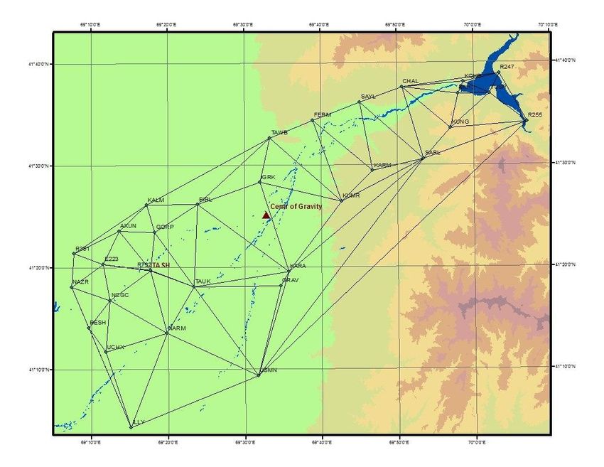
E3S Web of Conferences 227, 04002 (2021) https://doi.org/10.1051/e3sconf/202122704002
GI 2021

 Charvak dam with the height of 167 m has ended and started flowage of
 Brichmulla depression and filling of the Charvak reservoir [6].
 The GNSS geodetic network includes 31 stations (fig. 1), collected in campaign mode
 between 2009 and 2011 by researchers from the Institute of Seismology and the National
 Center of Geodesy and Cartography to study the modern deformations of the Earth’s
 surface using space geodetic methods.

 Fig.1. GNSS network of study area
 The region is well studied in terms of seismic activity and therefore a geodetic network
 was established here. The main task was to conduct research on the station’s velocities,
 deformations based on long-term GNSS measurements. The data were to become the basis
 for constructing a geodynamic model of the region's microplates. However, after 2011
 measurements were not taken due to both financial and organizational limitations.
 Therefore, in this work, we only consider the stability of the network, horizontal and
 vertical displacements caused by the influence of various datums. Stations installed with
 different spacing and varies from 5 km to 20 km. The GNSS data were observed over 6
 time periods (04.09.2009 – 27.09.2009; 05.11.2009 – 02.12.2009; 25.04.2010 –
 06.06.2010; 17.10.2010 – 6.11.2010; 19.04.2011 – 10.05.2011; 20.09.2011 – 6.11.2011)
 with the observation rate 10 s. Session duration for each station was 3 days. Ashtech Z-
 Surveyor dual-frequency receivers and ASH 701975-01 antennas were applied in all the
 surveys. Observations were carried out simultaneously by 12 receivers, and 6 were in
 stationary mode. Site positions and baselines for each epoch were estimated by
 aforementioned organizations with Trimble Total Control (TTC) software version 2.73.
 The free network solution was introduced for each campaign. For mathematical
 processing of satellite measurements, at least one point must be connected to a point on the
 international geodynamic network. Therefore, the absolute coordinates of the initial point
 NCGC were preliminary calculated relative to the international station TASH.
 Additionally, to tie the regional measurements to the global reference frame ITRF2008,
 data from continuously operating IGS permanent network stations (KIT3, MDVJ, POL2,

 2

E3S Web of Conferences 227, 04002 (2021) https://doi.org/10.1051/e3sconf/202122704002
GI 2021

 NSSP) were used. Coordinates of the test network estimated by six solutions have both
 different epochs and different datum. For accurate calculation of station displacement
 vectors, it is necessary to take into account the measurement errors that arise as a result of
 the choice of the reference system. As a result, “rotation” and “deformation” of the network
 arise. To eliminate the effect of visible “rotation” and “deformations” it is recommended to
 use the transformation methods. This study was aimed to compare the coordinate difference
 between the campaign’s epochs and referencing them into the first epoch of measurements
 by using 3D Helmert transformation method for the possibility of an accurate assessment of
 network deformations and strain accumulation computation.

 2 Materials and methods

 2.1 Datum investigation with 3-D Helmert transformation
 Usually, the processing of geodetic measurements to identify modern movements of the
 earth's crust is performed on relatively stable geological structures. However, for the study
 area, there is not yet a sufficiently accurate tectonic model and, accordingly, there is no sure
 confirmation that the points will remain stable. The territory of the Tashkent region is
 subject not only to modern tectonic movements, but also a change in the water level in the
 Charvak reservoir can be the cause of the induced disturbances of the Earth's surface. One
 of the solutions to the problem is the implementation in network processing of continuously
 working stations, for example IGS data. Taking into account that our network was
 processed relative to several high-precision stations of the IGS, in this study, all 31 points
 were used to perform the transformation procedure. Another reason was to look at how and
 where there will be more horizontal movement for further redefinition of the regional
 tectonic model.
 The network adjustment error is usually influenced by two factors: orientation and scale
 of the network. Therefore, a 7-parameter transformation method was chosen in the work to
 analyze deformation between two epochs and strain parameters in the geodetic network,
 three-dimensional conformal (it preserves shapes of objects) coordinate transformation is
 also known as seven-parameter similarity transformation was applied. It converts separate
 surveys into a common reference coordinate system and it can be thought of as a three-step
 process: scaling, rotation and translation. The seven parameters of the transformation
 between convertible (x,y) and reference (X,Y) systems (epochs) - one scaling (m), three
 rotations (RX, RY, RZ) and three rotations translations (TX, TY, TZ) can be determined
 uniquely with the minimum of three common points for both systems [7, 8]:

 X  T X   1 − RZ RY   x 
 Y = T  + (1 + m )  R (1)
 1 − RX   y 
    Y  Z  
  Z  i TZ   − RY RX 1   z  i

 When more than three stations are present, the solution is obtained by the conventional
 least square adjustment procedure and the equations system can be written in the matrix
 form:
 Ai dp= L + V (2)

 Where L-coordinate difference, V-vector of residuals. The design matrix Ai for station i
 of the are defined as

 3

E3S Web of Conferences 227, 04002 (2021) https://doi.org/10.1051/e3sconf/202122704002
GI 2021

 1 0 0 xi 0 0 y z 0 0 z − y
 (3)
=Ai 0 1 0 0 y 0 x 0 z −z 0 x
  
 0 0 1 0 0 z 0 x y y − x 0 

 The adjustment of the slightly overdetermined system (2) via normal equations yields
 the parameter vector dp of unknown transformation parameters (scaling, three rotations and
 
 three rotations translations) = � �

 dp = ( AT A) −1 AT L (4)

 Once parameters of the transformation are determined, the coordinates (x, y, z) are
 transformed to new (X, Y, Z)′ coordinate system using eq. (1). The coordinate values for all
 sessions were transformed to the topocentric coordinate system (E, N, U):

  En   − sin L0 cos L0 0  Xn − X0
 N  =  − sin B cos L − sin B0 sin L0 cos B0   Yn − Y0  (5)
  n  0 0  
 U n   cos B0 cos L0 cos B0 sin L0 sin B0   Z n − Z 0 
 where (X0,Y0,Z0) and (B0, L0) are geocentric and geodetic coordinates (latitude and
 longitude) respectively of the center of gravity of the network ( marked as red circle on
 fig.1). First epoch (Sept. 2009) of the measurement was choosing as reference for further
 calculations and the horizontal displacement vectors of pairs first – second (Nov. 2009),
 first − third (June 2010), first − fourth (Nov. 2010), first – fifth (May 2011) and first -six
 (Nov. 2011) epochs of each GNSS monitoring station was calculated as

 Rn = ( N n' − nn ) 2 + ( En' − en ) 2 (6)

 dU=
 n U n' − un height component variations will be used for estimation of the network
 vertical deformation. A software package in Delphi has been developed for the assessment
 of the datum differences between 2009 and 2011 by implementing the 3D Helmert
 transformation method.
 Data analysis was performed in the ArcGIS 10.1.

 2.2 Estimation of strain accumulation by finite element model
 The calculation of the network strain by the finite element method was used to assess
 the deformation effect. The principles and basics of finite element method are generally
 known and are described in numerous publications [9, 10]. In the first step, the network has
 been constructed of finite elements (triangles) based on the Delaunay triangulation (Green
 and Sibson, 1978) (fig.1). Local strain field was computed for each triangle in the network.
 The strain values (E) on the earth’s surface can be expressed in terms of displacements
 between adjacent stations at initial and final epochs (l0, l1) [11]:
 l − l0
 E=
 l0 (7)
 This equation is created for each baseline of a triangle. The coordinates of GNSS points
 were represented in the Mercator projection for calculating distances (radius-vectors)
 between the nearest stations.

 4

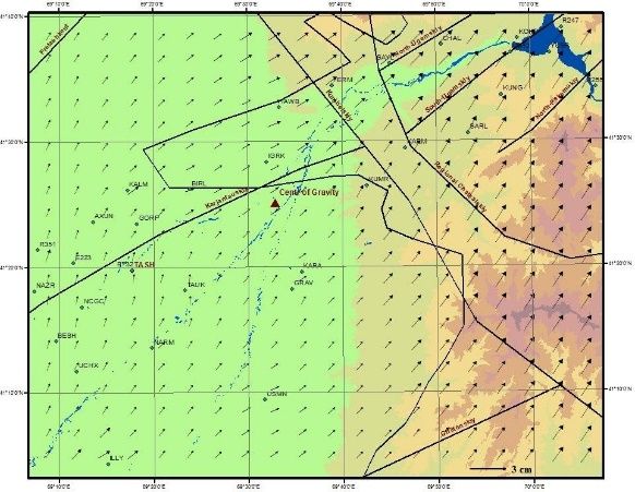
E3S Web of Conferences 227, 04002 (2021) https://doi.org/10.1051/e3sconf/202122704002
GI 2021

 Finally, all individual results are integrated for whole investigated region by creating
 homogeneous surface with the nearest neighbor interpolation method. It is based on
 comparison of the distribution of distance d between a point x and the nearest neighboring
 points y of a set of randomly distributed data [12]:
 ( , ) = ‖ − ‖ = �( − )( − ) = ((∑ ( − ))2 )1/2 (8)
 The method has been investigated and used in recent work for assessment of normal
 heights surface for Fergana valley territory in Uzbekistan [13]. It showed more reliable
 results than commonly used polynomial interpolation method for creating surface over the
 high mountains region.

 3 Results
 The transformation parameters translations (TX, TY, TZ), scale (m) and rotations ( ωX, ωY,
 ωZ) between the first-reference and subsequent (from second to sixth) epochs are given in
 the Table 1. The result revealed that there is significant translation and rotation in the
 network, while the scale of the network remains almost constant during two years period
 (from September 2009 to November 2011).
 Table 1. The transformation parameters between different epochs of measurements
 Epochs Period Tx, m Ty, m Tz, m m ωX, ωY, sec ωZ sec
 sec
 1−2 09.2009- -9.96 0.02 4.12 0.99 0.076 -0.294 0.185
 12.2009
 1−3 09.2009- -5.16 -2.04 -1.90 1.00 0.025 -0.028 0.160
 06.2010
 1−4 09.2009- 2.48 -5.53 6.20 0.99 0.258 -0.006 -0.110
 11.2010
 1-5 09.2009- -6.99 1.35 9.24 0.99 0.157 -0.295 0.106
 05.2011
 1-6 09.2009- 4.29 8.72 21.16 0.99 0.289 -0.112 -0.044
 11.2011

 The horizontal displacement vectors were calculated using the eq. 5 and, for a more
 visual representation of the deformation of the whole region, the values were interpolated
 over the study area (eq. 7). The presented in fig. 2a result demonstrate horizontal
 displacements of the network with rates between 2 cm and 21 cm during whole observation
 period (first and sixth epochs) from September 2009 to November 2011. Analysis of
 calculated displacement vectors has been carried out separately for different parts of the
 region. The investigated field was conditionally divided into three main parts. The first one
 belongs to the Charvak coastal zone (KOKB, NM12, YUSP, CHAL, KUNG, R247, R255,
 SAYL, SARL, KARM, FERM) and divided from the others by the Kumbel fault. The
 second and the third are separated from each other by the largest Karjantau depression and
 hereinafter called conditionally the Northern coastal zone of the Chirchik river (AXUN,
 BIRL, E223, GORP, IGRK, KALM, NAZR, R351, TAWB) and the Southern coastal zone
 of the Chirchik river (KUMR, GRAV, KARA, TAUK, R732, NARM, NCGC, BESH,
 UCHX, USMN, ILLY). It should be noted that deformations in the Chirchik river valley are
 less (about 1 cm) than in the coastal part.
 The stations located in Northern coastal part of the river have displacement rate from 4
 cm to 10 cm and the stations located in the Southern coastal zone have a displacement rates
 from 2 cm to 17 cm. Moreover, the stations located closely to a coastal part of the Charvak

 5

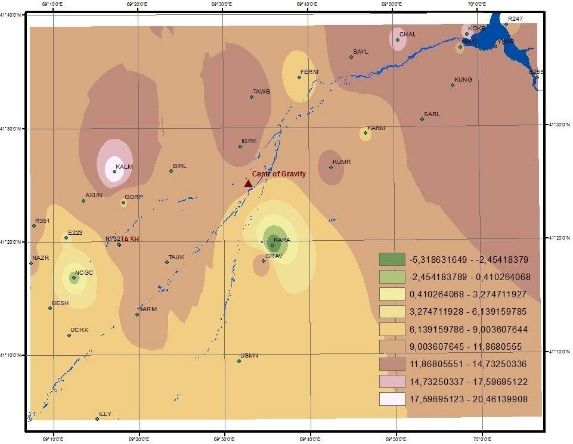
E3S Web of Conferences 227, 04002 (2021) https://doi.org/10.1051/e3sconf/202122704002
GI 2021

 reservoir (R247, NM12, R255, YUSP) have a maximum displacement rates in this zone
 between 13 cm and 20 cm. There is a tendency to rotational movement along the Kumbel
 and Karjantau faults (fig2a).
 The presented in fig. 2b result demonstrate vertical displacements of the network with
 rates between - 5 cm and 20 cm during the two years observation period. Station (KALM)
 located in this region shows relative to other stations a high rate of vertical displacement 20
 mm, the cause of which may mainly be instrumental (antenna information, et al.) errors
 than tectonic effects. Therefore, this station was excluded from further analysis. It can be
 concluded that for this region, horizontal displacements are a consequence of both tectonic
 and hydrological processes. While vertical deformations are the result of most tectonic
 phenomena

 a) b)
 Fig.2 Horizontal (a) and vertical (b) deformations of the network during 2009-2011
 The result revealed that there are significant horizontal displacements, therefore, it is
 necessary to estimate the strain accumulation regardless of the datum and the displacement
 vectors may be used to derive this parameter.

 Fig. 3. The map of strain values based on GNSS data over region

 6

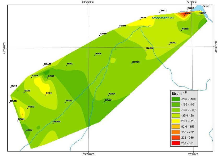
E3S Web of Conferences 227, 04002 (2021) https://doi.org/10.1051/e3sconf/202122704002
GI 2021

 Fig. 3 shows the principal strains rate distribution. Most of the area can be considered to
 be in a high compression (negative dilatation) strain state. Strain rate for the southwestern
 part near stations GRAV, KARA, AXUN, GORP as maximum value with -230×l0-8.
 Minimum values of extension are found in with a value of 10×l0-8 in flat areas. The results
 are very similar to the [5]: the strain rate at intersection of active faults Karzhantau, Kumbel
 and Ugam confirmed 80% of the value major shear stress caused by the tectonic
 movements of the whole region. On the contrary, remarkable positive dilatation strain is
 concentrated on the coastline of the water reservoir, where large strain is about 351×l0-8.
 The result clear demonstrates that, along strain caused by the tectonic movements, the water
 level variations in the reservoir is also a major factor determining the displacement and
 stability of the area.

 4 Conclusions
 The effect of the deformation processes in Tashkent region, was studied by strain
 deformation calculation with GNSS data. In this regard, as the first step, GNSS stations
 coordinates were transformed to a datum of the first epoch using the 3D Helmert
 transformation method, and the horizontal displacement vectors were determined for each
 station. The result revealed that there are significant horizontal displacements with a
 maximum value up to 20 cm in the network and vertical displacements with rates between -
 5 cm and 20 cm. The calculation of the network strain was used to assess the network
 deformation. The network has been constructed of finite elements (triangles) based on the
 Delaunay triangulation. We found that most of the Tashkent region can be considered to be
 in a high compression (negative dilatation) strain state confirmed, surely, of the value major
 shear stress caused by the tectonic movements of the whole region. On the contrary,
 remarkable positive dilatation strain is concentrated on the coastline of the water reservoir,
 where large strain is about 351×l0-8. We can conclude that more GNSS campaigns in
 combination with gravity measurements are needed in this area in order to better constrain
 the relatively small deformation rates.

 This work was carried out within the scientific and applied project FA-Atab-2018-57 of the
 Astronomical Institute of Uzbekistan with the financial support of the Ministry of Innovative
 Development of the Republic of Uzbekistan. We are very grateful to Institute of Seismology and
 National Center of Geodesy and Cartography, who organized GNSS experiments and made the data
 available to this study.

 References
 1. A. R. Yarmukhamedov. The morphostructure of the median Tien Shan and its
 relationship with seismicity. Tashkent: Fan, 163 (1988) (In Russian). https://www.geo-
 fund.am/files/library/1/15247392644395.pdf
 2. T. Rashidov, L. Plotnikova and S.Khakimova. Seismic hazard and building
 vulnerability in Uzbekistan // in Seismic Hazard and Building Vulnerability in Post-
 Soviet Central Asian Republics. edited by S.A. King, Vitaly I. Khalturin, B.E. Tucker.
 NATO ASI series. Vol.52. (1999)
 3. D. Giardini, G. Grünthal, K. M. Shedlock, and P. Zhang. The GSHAP Global Seismic
 Hazard Map. In: Lee, W., Kanamori, H., Jennings, P. and Kisslinger, C. (eds.):
 International Handbook of Earthquake & Engineering Seismology, International
 Geophysics Series 81 B, Academic Press, Amsterdam, 1233-1239 (2003)
 http://www.gfz-potsdam.de/GSHAP

 7

E3S Web of Conferences 227, 04002 (2021) https://doi.org/10.1051/e3sconf/202122704002
GI 2021

 4. T. U. Artikov, R. S. Ibragimov, T. L. Ibragimova, K. I. Kuchkarov, M. A. Mirzaev.
 Quantitative assessment of seismic hazard for the territory of Uzbekistan according to
 the estimated maximum ground oscillation rates and their spectral amplitudes.
 Geodynamics & Tectonophysics 9 (4), 1173–1188 (2018) doi:10.5800/GT‐2018‐9‐4‐
 0389.
 5. H. L. Hamidov. Identification of morphokinetic indicators of modern geodynamics of
 western Tiang Shan // Modern geodynamics of Central Asia and dangerous natural
 processes: quantitative research results: Materials of the All-Russian meeting and
 youth school on modern geodynamics (Irkutsk, September 23–29, 2012). - In 2-ht. -
 Irkutsk: IZSORAN, T. 2. 211 (2012)
 www.crust.irk.ru/images/upload/newsfond143/299.pdf
 6. M. Juliev, A. Pulatov, J. Hübl. Natural hazards in mountain regions of Uzbekistan: A
 review of mass movement processes in Tashkent province. International Journal of
 Scientific & Engineering Research, Vol. 8, Issue 2, February (2017)
 7. R. P. Wolf, and D. C. Ghilani. Adjustment computations: statistics and least squares in
 surveying and GIS. Wiley, New York, 347 (1997)
 8. I. Deniz, & H. Ozener. Estimation of strain accumulation of densification network in
 Northern Marmara Region, Turkey. Natural Hazards and Earth System Science,
 10(10), 2135–2143 (2010) https://doi.org/10.5194/nhess-10-2135-2010
 9. A. Dermanis. A method for the determination of crustal deformation parameters and
 their accuracy from distances. J. Geod. Soc. Japan, 40, 17-32 (1994)
 10. O.C. Zienkiewicz, R.L. Taylor, and J.Z. Zhu. The Finite Element Method: Its Basis
 and Fundamentals. 6th edition, Butterworth-Heinemann. 752 (2005)
 11. A.O. Agibalov, V.A. Zaytsev, A.A. Sentsov, A.S. Devyatkina. Assessment of the
 influence of modern crustal movements and the recently activated Precambrian
 structural plan on the relief of the Lake Ladoga region (the southeastern Baltic Shield).
 Geodynamics & Tectonophysics 8 (4), 791–807 (2017) doi:10.5800/GT-2017-8-4-
 0317
 12. P. D. Dumitru, M. Plopeanu, and D. Badea. Comparative Study Regarding the Methods
 of Interpolation. In: Proceedings of the 1st European Conference of Geodesy &
 Geomatics Engineering (GENG '13), 32-37 (2013)
 http://www.wseas.us/elibrary/conferences/2013/Antalya/GENG/GENG-00.pdf.
 13. D. Fazilova, H. Magdiev. Comparative study of interpolation methods in development
 of local geoid. International Journal of Geoinformatics, - V.14, №1. 29–33 (2018)
 http://journals.sfu.ca/ijg/index.php/journal/article/view/1114/599

 8