Modeling symbiotic biological nitrogen fixation in grain legumes globally with LPJ-GUESS (v4.0, r10285) - GMD
←
→
Page content transcription
If your browser does not render page correctly, please read the page content below

Geosci. Model Dev., 15, 815–839, 2022
https://doi.org/10.5194/gmd-15-815-2022
© Author(s) 2022. This work is distributed under
the Creative Commons Attribution 4.0 License.

Modeling symbiotic biological nitrogen fixation in grain legumes
globally with LPJ-GUESS (v4.0, r10285)
Jianyong Ma1 , Stefan Olin2 , Peter Anthoni1 , Sam S. Rabin1 , Anita D. Bayer1 , Sylvia S. Nyawira3 , and Almut Arneth1,4
1 Institute of Meteorology and Climate Research-Atmospheric Environmental Research, Karlsruhe Institute of Technology,
82467 Garmisch-Partenkirchen, Germany
2 Department of Physical Geography and Ecosystems Science, Lund University, 22362 Lund, Sweden
3 International Center for Tropical Agriculture (CIAT), ICIPE Duduville Campus, P.O. Box 823-00621, Nairobi, Kenya
4 Institute of Geography and Geoecology, Karlsruhe Institute of Technology, 76131 Karlsruhe, Germany

Correspondence: Jianyong Ma (jianyong.ma@kit.edu)

Received: 30 July 2021 – Discussion started: 15 September 2021
Revised: 8 December 2021 – Accepted: 11 December 2021 – Published: 28 January 2022

Abstract. Biological nitrogen fixation (BNF) from grain          1   Introduction
legumes is of significant importance in global agricultural
ecosystems. Crops with BNF capability are expected to sup-
port the need to increase food production while reducing         The agricultural sector is the main contributor to anthro-
nitrogen (N) fertilizer input for agricultural sustainability,   pogenic nitrous oxide (N2 O) emissions (Reay et al., 2012;
but quantification of N fixing rates and BNF crop yields         Tian et al., 2020) and a key nitrate pollution source to fresh-
remains inadequate on a global scale. Here we incorporate        water systems (Moss, 2008), mostly due to the intensive use
two legume crops (soybean and faba bean) with BNF into           of synthetic nitrogen (N) fertilizer and animal manure (Lu
a dynamic vegetation model LPJ-GUESS (Lund–Potsdam–              and Tian, 2017). This trend has been amplified by the ex-
Jena General Ecosystem Simulator). The performance of this       pansion of agricultural land to provide food for a growing
new implementation is evaluated against observations from        population and changing dietary patterns (FAO, 2018). The
a range of water and N management trials. LPJ-GUESS              use of crops with biological N fixation (BNF) capability in
generally captures the observed response to these manage-        agriculture has been discussed as one option to address the
ment practices for legume biomass production, soil N up-         conflict between the need to increase food production and
take, and N fixation, despite some deviations from obser-        the associated environmental problems of N loss (Becker,
vations in some cases. Globally, simulated BNF is domi-          et al., 1995; Fageria, 2007; Northup and Rao, 2016). N-
nated by soil moisture and temperature, as well as N fer-        fixing crops, like grain and forage legumes, not only provide
tilizer addition. Annual inputs through BNF are modeled to       protein-rich food for the human population and farmed ani-
be 11.6 ± 2.2 Tg N for soybean and 5.6 ± 1.0 Tg N for all        mals (Voisin et al., 2014; Stagnari et al., 2017), but they are
pulses, with a total fixation of 17.2 ± 2.9 Tg N yr−1 for all    also directly useable as “green manure”, reducing the amount
grain legumes during the period 1981–2016 on a global scale.     of chemical N fertilizer required in agricultural systems (Liu
Our estimates show good agreement with some previous sta-        et al., 2011; Meena et al., 2018).
tistical estimates but are relatively high compared to some         Soybean (Glycine max L.), with its countless and varied
estimates for pulses. This study highlights the importance of    uses, is now one of the most widely grown crops in the world
accounting for legume N fixation process when modeling C–        because of attractive cash return from its grain yield (FAO-
N interactions in agricultural ecosystems, particularly when     STAT, 2021). There are concerns about the sustainability of
it comes to accounting for the combined effects of climate       soybean production, in particular because of its links to de-
and land-use change on the global terrestrial N cycle.           forestation and loss of native vegetation in the Amazon and
                                                                 other areas of South America (Fehlenberg et al., 2017; Heil-
                                                                 mayr et al., 2020). Other grain legumes, such as faba bean

Published by Copernicus Publications on behalf of the European Geosciences Union.
816                                                                  J. Ma et al.: Modeling biological N fixation with LPJ-GUESS

(Vicia faba L.), chickpea (Cicer arietinum L.), and cowpea               ments demonstrating that the energy consumption required
(Vigna unguiculata L.), play an important role in improv-                for BNF is far larger than soil mineral N uptake (Ryle et
ing soil quality as green manure when they are rotated or                al., 1979; Harris et al., 1985; Macduff et al., 1996). In several
used as intercrops between cereals depending on the region               other models, root substrate C concentration was adopted as
(Williams et al., 2014; Denton et al., 2017). In comparison to           an alternative to represent the C demand of N fixation (e.g.,
non-legume plants, using legumes as green manure is more                 Thornley and Cannell, 2000; Yu and Zhuang, 2020). Only a
effective to build up or maintain soil fertility, as they not only       few models assume that such a consumption can be assessed
increase soil organic matter when adding their biomass to                directly against C acquired in photosynthesis, in which the
soils, but also add extra N into the soil as a result of their           C cost per unit of fixed N is defined as either a constant of
symbiotic association with bacteria (Peoples et al., 2009;               6 kg C kg N−1 (Boote et al., 2008; Meyerholt et al., 2016)
Ciampitti and Salvagiotti, 2018). The enriched soil N and                or a dynamic function of soil temperature ranging between
soil organic carbon contents jointly support growth and pro-             7.5 and 12.5 kg C kg N−1 (Houlton et al., 2008; Fisher et
ductivity in subsequent crops (Jensen et al., 2012; Hajduk               al., 2010).
et al., 2015). Much experimental evidence has indicated that                 The global production and consumption of grain legumes
grain legume biomass increases linearly with an increasing               have greatly increased over recent decades (FAOSTAT,
BNF rate (Salvagiotti et al., 2008; Unkovich et al., 2010;               2021). Accurately representing and quantifying the dynamic
Córdova et al., 2019) and that the N benefit to soil fertility           process of biological N fixation in models is important for
from green manure is closely correlated with N fixation ca-              better understanding grain legumes’ contribution to food se-
pacity, assuming that the entire legume plant is tilled into the         curity and agriculture sustainability, particularly in the con-
soil (Fageria, 2007; Meena et al., 2018). Estimating the rate            text of global environmental change. However, because of in-
of BNF is thus important not only for an accurate prediction             adequate information on the environment and crop manage-
of grain legume production but also for a better understand-             ment, as well as the missing or incomplete BNF mechanism
ing of where and to what degree N loss (i.e., N leaching and             in models (e.g., C cost as mentioned above), current simu-
gaseous N emission) in cropland systems can be reduced by                lation of grain legume N fixation and its yield is still very
partially or fully replacing chemical N fertilizer with legume           weak, especially when it comes to global-scale modeling.
green manure.                                                                Thus, in this study, by accounting for the importance
   Although grain legumes’ BNF rates can be measured at                  of soybean in overall agriculture and trade, as well as the
field sites and in controlled environments, ecological models            higher N fixation capacity of faba bean compared to other
are needed for understanding and quantifying the rate of BNF             pulses (Peoples et al., 2009; Unkovich et al., 2010; Denton et
on larger spatial scales and longer temporal perspectives. In            al., 2017; Liu et al., 2019), we implement these two grain
many process-based crop models, a common method of rep-                  legumes with BNF into a process-based vegetation model
resenting BNF is to use a pre-defined potential or maximum               (LPJ-GUESS; Smith et al., 2014; Olin et al., 2015). Processes
N fixation rate that is adjusted by limiting environmental fac-          are added to LPJ-GUESS to estimate the symbiotic relation-
tors (Liu et al., 2011). The potential N fixation rate is then           ship between legumes and bacteria, also taking into account
estimated either from plant nodule, root, and aboveground                the plant C cost of BNF. Model results are extensively eval-
biomass (e.g., Boote et al., 2008; Corre-Hellou et al., 2009;            uated with worldwide site-level observed data and compared
Wu et al., 2020) or from plant N demand status (e.g., Ca-                against country-level yield statistics, as well as continent-
belguenne et al., 1999; Robertson et al., 2002), varying with            level BNF rates. The model-based and large-scale quantifi-
plant life cycle. Environmental constraining factors, such as            cation of the N fixation capacity in legumes provides a scien-
soil temperature, water availability, soil mineral N concen-             tific foundation for predicting the present and future N cycle
tration, and plant growth stage, are mostly taken into account           in agro-ecosystems, allowing recommendations for fertilizer
(Liu et al., 2011; Chen et al., 2016). The big challenge in              N application under different climatic conditions in legume-
modeling legume BNF is that the process of symbiotic N fix-              based farming systems.
ation is always accompanied by the cost of fixed total photo-
synthetic carbon (C) to maintain legume symbiotic growth,
activity, and reserves, which may be around 4 %–16 % of C                2     Methods
(Kaschuk et al., 2009). Such a photosynthetic consumption
strength would result in productivity loss if the photosynthe-           2.1    Model description
sis rate did not increase to compensate for the cost (Kaschuk
et al., 2010). In most models C cost mechanisms have not                 LPJ-GUESS is a process-based dynamic vegetation model
been implemented into N fixation, consistent with the as-                that simulates carbon and nitrogen (C–N) dynamics at scales
sumption that the plant N uptake from soils does not cost car-           typically ranging from regional to global (Smith et al., 2014).
bon (e.g., Cabelguenne et al., 1999; Robertson et al., 2002;             The model represents vegetation and soil dynamic processes
Corre-Hellou et al., 2009; Drewniak et al., 2013; Von Bloh               as well as their interactions in response to changes in the en-
et al., 2018; Wu et al., 2020), despite many field experi-               vironment and management, such as climate, CO2 concentra-

Geosci. Model Dev., 15, 815–839, 2022                                                      https://doi.org/10.5194/gmd-15-815-2022
J. Ma et al.: Modeling biological N fixation with LPJ-GUESS                                                                     817

tion, soil physical properties, N deposition, and N fertiliza-      where DS is crop development stage ranging from 0 to 2
tion. Three land-use types are included in the model: natural       (DS = 0, sowing; DS = 1, flowering; DS = 2, harvest); fphu
vegetation, pasture, and cropland. Vegetation on natural land       is the fraction of today’s accumulated heat units to the total
is represented as the establishment, growth, and mortality of       heat requirement; fphuanthesis is the threshold of fphu when
12 plant function types (PFTs). Pastures are simulated by           anthesis starts, below (above) which crop growth belongs to
competing C3 and C4 grasses, in which 50 % of aboveground           the vegetative (reproductive) stage; and a and b are the linear
biomass is annually harvested to account for the effects of         regression coefficients, varying between the vegetative and
grazing (Lindeskog et al., 2013). Crops in LPJ-GUESS are            reproductive phases. The values of a and b, as well as the
described by crop functional types (CFTs), which differ in          crop-specific base temperature (◦ C) to estimate the accumu-
their C allocation scheme, morphological traits, and heat sum       lated heat units, are both given in Table S1 in the Supplement.
requirement for growth. At present, four CFTs are repre-                The daily fraction of assimilate allocation to leaves, stems,
sented in the C–N version of LPJ-GUESS: two temperate C3            and roots is an important process before storage organs are
crops with sowing carried out in spring and autumn, a trop-         formed. The assimilate invested in roots can help crops over-
ical C3 crop (representing rice), and a C4 crop (representing       come water or nutrient limitation when they suffer from
maize). Sowing dates on a large scale are determined dynam-         stress in the vegetative stage, whereas new assimilate in-
ically in the model based on local climatology in each grid         vested in leaves generally gives a highly efficient return from
cell with five seasonality types represented (a combination         the photosynthesis product (Penning de Vries et al., 1989).
of temperature- and precipitation-limited behaviors; Waha           Unlike cereal crops, nodulated plants, particularly soybeans,
et al., 2012), and crops are harvested once each year when          are more likely to achieve a higher photosynthesis rate and
prescribed heat sum requirements are fulfilled (Lindeskog et        delay leaf senescence due to the continued N supply from
al., 2013). Multi-cropping systems within a year are not yet        biological N fixation (Abu-shakra et al., 1978; Kaschuk et
implemented in the model. The recent representation of crops        al., 2010). A precise representation of assimilate partitioning
includes the incorporation of soil N transformation (Tian et        to the plant organs when modeling BNF in grain legumes is
al., 2020) together with a C–N allocation for crops operating       especially important considering the high C cost from fixing
on a daily time step (Lindeskog et al., 2013; Olin et al., 2015).   N from the atmosphere. Productivity loss would be simulated
Cropland management options for global-scale application            if the leaf photosynthesis rate did not increase to compensate
include irrigation, tillage, N application, cover crop grass be-    for the costs (Macduff et al., 1996; Kaschuk et al., 2009).
tween the main growing seasons, and residue retention (Pugh             Following Olin et al. (2015), relationships between assim-
et al., 2015; Olin et al., 2015). In this study, soybean is simu-   ilate allocation to legume organs were established based on
lated as one additional crop because of its large importance as     the data from Penning de Vries et al. (1989) and Boote et
a food, fodder, and oil crop, and the parametrization of faba       al. (2002). We fitted the allocation functions using a Richards
bean is representative for the group of pulses in general. The      logistic growth curve (Eq. 2, Richards, 1959) to model the al-
model schematic and other calculations including the C cy-          location to each organ dynamically and separately. For each
cle and the N cycle follow an earlier version of LPJ-GUESS          allocation function fi (see Eqs. 3–5 below),
(Smith et al., 2014; Wårlind et al., 2014; Olin et al., 2015).
                                                                                      bi − ai
                                                                    fi = a i +                        ,                          (2)
2.2   Updated daily carbon allocation parameters                                 1 + e−Ci ×(DS−di )
                                                                    where DS is crop development stage, and ai , bi , ci , and di
Similar to most ecosystem and crop models, LPJ-GUESS                are fitting coefficients for the three functions (specific values
adopts crop-specific accumulated heat requirements to model         given in Table S1).
plant growth development, and crops are allowed to adapt to            Maintaining BNF in the reproductive stage (i.e., after an-
the local climate by dynamically adjusting the heat require-        thesis; DS > 1) would reduce the flow of carbon assimilation
ments to different climatic zones (Lindeskog et al., 2013).         to storage organs. We adjusted the allocation functions from
To better represent C and N allocation in various phenologi-        Olin et al. (2015) so that the model allowed a dynamic adap-
cal phases, Olin et al. (2015) defined crop development stage       tation of the allocation to grain over the seed-filling period in
by considering the effects of temperature, vernalization days,      response to BNF cost (see Eqs. 3–5 for details).
and photo-period following Wang and Engel (1998). In this
study, we assume that the grain legume development stage is         2.2.1   Yield vs. the whole plant
linearly correlated with its accumulated heat units according
to the field-based soybean experiments described in Irmak et        After anthesis (DS > 1), most assimilates are allocated and
al. (2013). It is estimated as                                      re-translocated from the vegetative organs to the grains. Dur-
                                                                    ing the late seed-filling period (DS ≥ d1 , see Eq. 3), we as-
       (                                                           sumed that the fraction of carbon allocated to yield would in-
           aveg + bveg × fphu    fphu ≤ fphuanthesis                crease to partly compensate for the productivity loss caused
DS =                                                    ,   (1)
           arep + brep × fphu    fphu > fphuanthesis                by spending on N fixation at the cost of reducing the flow

https://doi.org/10.5194/gmd-15-815-2022                                                    Geosci. Model Dev., 15, 815–839, 2022
818 J. Ma et al.: Modeling biological N fixation with LPJ-GUESS
of carbon to leaves and stem (see Eq. 4). We established the (6).
ratio of the allocation to yield relative to the whole plant as
Pyield = f1
Pyield Pleaf = f2 × (1 − f1 ) × (1 − f3 )
f1 = (7)
Pveg + Pyield
Pstem = (1 − f1 ) × (1 − f2 ) × (1 − f3 )
Proot = f3 × (1 − f1 )
b1 −a1
a1 + DS < d1
1+e−c1 ×(DS−d1 )
=
b1 −a1 , (3)
a1 + −c1 ×(DS−d1 ) × (1 + PBNFcost ) DS ≥ d1 Partitioning functions are plotted for soybean in Fig. 1b and
1+e
for faba bean in Fig. S1 in the Supplement. Significant dif-
where Pyield and Pveg are the fraction of carbon allocated to ferences in allocation patterns can exist between cultivars.
yield and vegetative organs, respectively, ranging from 0 to Compared to cereals (Olin et al., 2015), we found that grain
1; PBNFcost is the proportion of net primary production (NPP) legumes are more likely to allocate more assimilate to leaves
used for BNF to today’s total NPP; and d1 is the fitting co- not only in partitioning proportion but also in the length of
efficient representing the DS of the maximum growth rate of allocation time, probably corresponding to their higher leaf
grain (d = 1.41 for soybean and 1.46 for faba bean, see Ta- activities in response to N fixation (Kaschuk et al., 2010).
ble S1).
2.3 Representation of BNF
2.2.2 Leaf vs. shoot vegetative organs
Fixing N from the atmosphere and N uptake from soils rep-
Similarly, the ratio of leaf vs. shoot vegetative allocation is resents two N sources for grain legumes to meet their total
specified as plant N demand. The latter has a higher priority for plants
because the process is less energy-consuming than N fixa-
Pleaf tion (Ryle et al., 1979; Macduff et al., 1996). Following on
f2 =
Pveg − Proot this idea, in LPJ-GUESS, N fixation will only be triggered
b2 −a2
DS < d1 when the following two assumptions are valid at the same
a2 + 1+e−c2 ×(DS−d2 )
=
, (4) time (Fig. 2): (1) if today’s plant growth still suffers from N
b2 − a2
a 2 + − PBNFcost DS ≥ d1 limitation after N uptake from soils (i.e., the N deficit, plant
1 + e−c2 ×(DS−d2 )
N demand minus soil N uptake, is greater than zero). The
plant will then be allowed to fix N from the atmosphere to
where Pleaf and Proot are the fraction of carbon allocated to
fill the N deficit. (2) Since N fixation is strongly related to
leaf and root, respectively. The fitting function of leaf vs.
photosynthetic assimilate due to its high energy consump-
shoot vegetative organs in soybean is given in Fig. 1a.
tion, BNF in the model is assumed to take place only when
2.2.3 Root vs. vegetative organs today’s NPP is positive so that adequate C supply can be pro-
vided to meet the BNF cost.
When a plant experiences water or nutrient stress, it invests Modeling the BNF rate is adapted from previously pub-
more assimilate to roots relative to shoot vegetative organs lished methods (e.g., CROPGRO, EPIC, APSIM; see Liu et
(Penning de Vries et al., 1989). We implemented dynamic al., 2011) in that it considers (1) the potential N fixation rate,
increases in the allocation to roots during the late seed-filling (2) the limitation of temperature, (3) soil water status, and
period to help legumes cope with the C loss from BNF cost (4) the crop growth stage as
and established the relationship between the allocation to
root and that to vegetative organs as Nfix = Nfixpot × fT × fW × fDS , (8)
Proot where Nfix is the N fixation rate; Nfixpot is the potential N
f3 =
Pveg fixation rate; and fT , fW , and fDS are limitations (ranging 0
b3 −a3
DS < d1 to 1) on BNF by soil temperature, soil water availability, and
a3 + 1+e−c3 ×(DS−d3 )
=
b3 − a3
. (5) crop development stage function, respectively.
a3 +
−c ×(DS−d )
+ (1 − f1 ) × PBNFcost DS ≥ d1 The definition of the potential N fixation rate in some stud-
1+e 3 3
ies is based on the strong relationship between N fixation
In addition, carbon partitioning to vegetative organs (Pveg ) and either nodule size, biomass (Weisz et al., 1985; Voisin et
can be calculated by subtracting the reproductive allocation al., 2003), or root dry matter (Soussana et al., 2002; Voisin
(i.e., Pyield ) from the whole plant as et al., 2007). Due to the difficulties in measuring both nod-
ules and roots in the field directly, some studies also adopt
Pveg + Pyield = 1 ⇒ Pveg = 1 − Pyield = 1 − f1 . (6) shoot biomass to replace nodule or root biomass based on
the empirical relationship between these two variables (Yu et
Finally, we can achieve dynamic carbon allocation to the al., 2002; Corre-Hellou et al., 2009; Wu et al., 2020). In our
plant organs over the growing season by combining Eqs. (3)– implementation, since the nodulation process of legumes has
Geosci. Model Dev., 15, 815–839, 2022 https://doi.org/10.5194/gmd-15-815-2022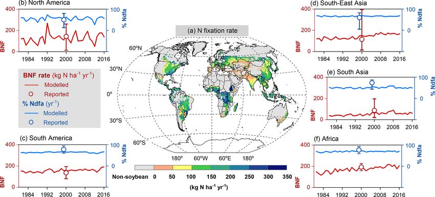
J. Ma et al.: Modeling biological N fixation with LPJ-GUESS 819
Figure 1. The organ’s relative allocation (a) and assimilate partitioning (b) to roots, leaves, stem, and yields for soybean. Solid lines represent
the fitted Richards functions in this study, and dashed lines are the allocation scheme from Penning de Vries et al. (1989). f2 in (a) denotes
leaf relative allocation to shoot vegetative organs (Eq. 4), whereas f3 is root relative allocation to vegetative organs (Eq. 5).
not yet been implemented in LPJ-GUESS, Nfixpot is assumed model (0–50 cm), Tmin (Tmax ) is the minimum (maximum)
to be proportional to root dry matter: temperature below (above) which N fixation stops, and ToptL
and ToptH are the lower and higher optimal temperatures
Nfixpot = Nmaxfixpot × DMroot , (9) within which N fixation is not limited by temperature. The
where Nmaxfixpot is the maximum nitrogen fixation rate values of these four temperature thresholds vary among
of roots (g N g−1 root DM), and DMroot is root dry legume crops and are given in Table 1.
matter (g root DM m−2 ). Since the experimental parameter In addition to temperature, soil water content is a major
Nmaxfixpot is strongly related to the effectiveness of rhizo- factor controlling the rate of N fixation (Srivastava and Am-
bial strains and varies widely between species and sites, it basht, 1994). Too little water strongly inhibits BNF due to
is not easy to obtain the parameter for each legume crop. impacts of drought stress on nodule nitrogenase activity (Ser-
In this study, we assume that legumes are either inocu- raj et al., 1999; Marino et al., 2007). Although oxygen is
lated or there are high enough populations of strains in the needed to support the respiration of legume roots and bac-
soil that Nmaxfixpot is not constrained by the effectiveness teria in the nodules, nitrogenase is more active in anoxic,
of rhizobia. Here Nmaxfixpot is assumed to be a constant as waterlogged environments (Jiang et al., 2021). A linear wa-
0.03 g N g−1 root DM for both grain legumes as a moderate ter limitation function is thus incorporated into LPJ-GUESS
value taken from the literature (Soussana et al., 2002; Ecker- (Wu and McGechan, 1999) and is represented as
sten et al., 2006; Boote et al., 2008).
Soil temperature is a controlling factor for both micro- 0
Wf ≤ Wa
bial activities and plant growth. For soybean, 20–35 ◦ C has fW = ϕ1 + ϕ2 × W f Wa < Wf < Wb , (11)
been found to be optimal for nitrogenase activity and for faba
1 Wf ≥ Wb
bean the optimal soil temperature can range from 16–25 ◦ C
(Boote et al., 2008). The influence of soil temperature on where Wf is relative soil water content in the topsoil layer
legume BNF is represented in the model as a four-threshold- (0–50 cm) ranging from 0 to 1, ϕ1 and ϕ2 are empirical co-
temperature function: efficients, Wa is the threshold of Wf below which N fixation
is fully restricted by soil water deficit, and Wb is the value
0 (T < Tmin or T > Tmax ) above which N fixation is not inhibited by soil water content.
T − Tmin The values of the parameters are shown in Table 1.
Tmin ≤ T < ToptL
ToptL − Tmin The influence of plant growth stage on legume BNF rate is
fT = , (10)
1 ToptL ≤ T ≤ ToptH taken into account in very few models; the process is gener-
ally stopped forcibly after the crop reaches a certain develop-
Tmax − T
ToptH < T ≤ Tmax
ment stage. For example, in the CROPGRO model (Boote et
Tmax − ToptH
al., 2008), N fixation in soybean starts in the second trifolio-
where T is soil temperature (◦ C) at a depth of 25 cm rep- late stage and continues until the end of physiological matu-
resenting the mean temperature of the topsoil layer in the rity, whereas it ceases at the middle of the seed-filling period
https://doi.org/10.5194/gmd-15-815-2022 Geosci. Model Dev., 15, 815–839, 2022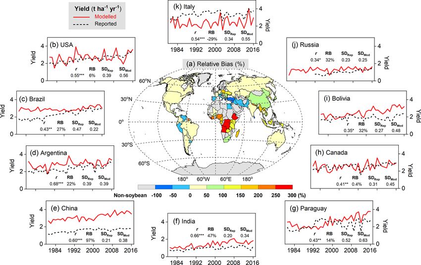
820 J. Ma et al.: Modeling biological N fixation with LPJ-GUESS
in the EPIC model (Cabelguenne et al., 1999). Much experi- leaf and stem, respectively (see Eq. 7 for details). A flowchart
mental evidence has indicated that the N fixed by legumes of the BNF scheme in LPJ-GUESS is shown in Fig. 2.
varies widely among crop growth stages, with the largest
BNF rate observed between the late vegetative phase and the 2.4 Experimental setup
early seed-filling period (Santachiara et al., 2017; Córdova
et al., 2020; Ciampitti et al., 2021). In this study, a specific Field-based data from the literature, together with global
function, similar to the temperature response function, is thus yield statistics from legume-producing countries and region-
implemented in the BNF scheme to represent the variation of level N fixation data from published sources, were compared
N fixation with the course of the legume life cycle: to model runs to examine performance in simulating yields
and BNF rate from the site scale to a larger region.
fDS In order to build up cropland soil C and N pools, all
0 (NDS < NDSmin or NDS > NDSmax ) simulations were initialized with a 500-year spin-up using
NDS − NDSmin
NDSmin ≤ NDS < NDSoptL
atmospheric CO2 from 1901 combined with repeating de-
NDSoptL − NDSmin
=
1 NDSoptL ≤ NDS ≤ NDSoptH
(12) trended 1901–1930 climate from GSWP3-W5E5 (Dirmeyer
et al., 2006; Lange, 2019; Cucchi et al., 2020). The crop-
NDSmax − NDS
NDSoptH < NDS ≤ NDSmax
NDSmax − NDSoptH land fraction linearly increased from zero to the first historic
value (1901) during the last 30 years of spin-up. Monthly at-
where NDS is normalized crop development stage ranging mospheric N deposition (NHx , NOy ) was used as simulated
from 0 to 1 (0, sowing; 0.5, flowering; 1, harvest), NDSmin is by CCMI (NCAR Chemistry–Climate Model Initiative). The
the time before which there is no N fixation due to inadequate value was interpolated to 0.5◦ × 0.5◦ from the original res-
nodulation, NDSmax is the time after which N fixation sus- olution (1.9◦ × 2.5◦ ) to match the resolution of the climate
pends due to nodule senescence, and NDSoptL and NDSoptH data (Tian et al., 2018). Below, the setup of the different ex-
define the period within which the legume BNF rate is not periments is explained in detail.
inhibited by development stage. The values of the parame-
ters for two grain legumes are derived from the literature and 2.4.1 Model evaluation at site scale
listed in Table 1.
In addition to the environmental limitation factors, the To evaluate the model’s ability to simulate BNF rate and
amount of daily NPP also affects N fixation in the model. yields, field-based N fixation trials with detailed measure-
The NPP requirement for BNF cost is computed based on ments of soil N uptake, biomass, and N mass allocation were
the estimated N fixation rate (Nfix , Eq. 8) by multiplying collected from the published literature. This dataset com-
the C cost per unit fixed N, which is assumed to be a fixed prised 17 soybean and 7 faba bean sites located between
value of 6 g C g−1 N as a moderate value taken from previous ∼ 33◦ S and ∼ 53◦ N (Fig. 3). In these trials, BNF response
studies (Ryle et al., 1979; Patterson and Larue, 1983; Boote to various management practices (such as N fertilizer ad-
et al., 2008; Kaschuk et al., 2009). The NPP cost to main- dition and irrigation) were investigated. Details about these
tain BNF is released as CO2 to the atmosphere and mod- sites – their geographic coordinates, BNF trials, and the years
eled as part of the autotrophic respiration of the soil (Fig. 2). of available data, as well as corresponding site-specific plant
Since the fixed N is partly transported to plant leaves and traits (e.g., specific leaf area and grain C : N ratio) – are pro-
continues to support photosynthesis, the plant may get addi- vided in Table S2.
tional C profits from the investment of BNF by enhancing In some field experiments, BNF rate and/or soil N uptake
the leaf N content that optimizes the carboxylation capacity are not directly reported in the literature, so we estimated
(Vmax ) (Kull, 2002). Following on this idea, another assump- these values as
tion adopted in this study is that at most 50 % of today’s NPP
BNFobs = %Ndfa × Nplant
can be used for N fixation before the crops reach the devel- (14)
SoilNuptakeobs = (100 − %Ndfa) × Nplant ,
opment stage of grain maximum growth rate (DS < d1 , see
Eq. 13). After this the maximum proportion of today’s NPP where %Ndfa is the proportion of plant N derived from the
used for BNF cost is dynamically reduced and assumed to be atmosphere (ranging 0–100), representing the contribution of
the fraction of carbon allocation to leaves and stem: N fixation to the plant total N uptake, and Nplant is the amount
MAXNPPBNFcost of N accumulated in the plant (kg N ha−1 ), defined as either
( the shoot or the whole plant N mass, depending on the mea-
0.5 DS < d1 surement method adopted in the experiment.
= , (13)
Pleaf + Pstem = (1 − f1 ) × (1 − f3 ) DS ≥ d1 In general, grain yields, plant tissue dry mass, and N mass,
together with %Ndfa, soil N uptake, and N fixation, are
where MAXNPPBNFcost is the maximum proportion of to- widely measured variables in field-based BNF trials (see Ta-
day’s NPP used for N fixation varying from 0–0.5, and Pleaf ble S2). These data were chosen as our target variables used
and Pstem are the fraction of carbon (i.e., NPP) allocated to for model evaluation. In addition, to convert plant C mass
Geosci. Model Dev., 15, 815–839, 2022 https://doi.org/10.5194/gmd-15-815-2022
J. Ma et al.: Modeling biological N fixation with LPJ-GUESS                                                                       821

Figure 2. Representation of the N fixation route used in grain legumes in LPJ-GUESS. Today’s N deficit is calculated as the difference
between plant N demand and soil mineral N uptake. Nfix in dotted boxes represents intermediate values.

to dry matter, a conversion factor of 2.0 was used (Smith et         air temperatures (maximum, minimum, and mean), precip-
al., 2014). Dry weight was converted to wet weight by as-            itation, and solar radiation were used from GSWP3-W5E5
suming a water fraction of 0.13 in the grain legumes (Cór-           (Dirmeyer et al., 2006; Lange, 2019; Cucchi et al., 2020),
dova et al., 2019).                                                  chosen for the 0.5◦ ×0.5◦ grid cell representative for each ex-
   Since specific leaf area (SLA) and target grain C : N ratio       perimental site. We compared model-required input variables
play a very important role in determining N uptake and N re-         from GSWP3-W5E5 with observations at three sites, finding
translocation to grain during seed-filling in the model (Olin et     that the gridded climate data had fairly good agreement with
al., 2015), we implemented two simulations to explicitly ex-         weather records in the field, despite some solar radiation de-
plore model performance across all sites. For “site-specific”        viations between two datasets for individual days over the
simulations, the reported SLA and grain C : N ratio listed in        experimental period (Fig. S2). There was no information on
Table S2 were adopted for the simulation (for sites for which        land-use and management practices in years preceding the
these were available). For “global uniform” parameter sim-           experiments at most sites. Therefore, to maintain soil N and
ulations, SLA was set to 40 and 45 m2 kg−1 C (Penning de             C pools in equilibrium after model spin-up, we decided to
Vries et al., 1989), and the target grain C : N ratio was rep-       implement a common cropping system of maize–legume ro-
resented as a constant of 8 for soybean and 10 for faba bean         tation annually from 1901 to the year before the trial start,
(Kattge et al., 2020). These values were also used for global-       with no N fertilizer applied to legumes. Over the trial pe-
scale simulations.                                                   riod, the management practices were implemented accord-
   Due to the unavailable information on weather data at the         ing to information provided in the literature (Table S2). In
majority of the sites evaluated, gridded daily climate data for      addition, site-specific soil physical properties, such as frac-

https://doi.org/10.5194/gmd-15-815-2022                                                    Geosci. Model Dev., 15, 815–839, 2022

822                                                                     J. Ma et al.: Modeling biological N fixation with LPJ-GUESS

Table 1. Overview of BNF-related variables and parameters used in the model for soybean and faba bean.

 Parameter     Description                                                 Soybean       Faba bean      Unit                   Reference
 N deficit     plant N demand minus soil N uptake                          dynamic       dynamic        g N m−2 d−1
 NPP           net primary productivity                                    dynamic       dynamic        g C m−2 d−1
 Nmaxfixpot    maximum nitrogen fixation rate of roots                     0.03          0.03           g N g−1 root DM        Soussana et al. (2002),
                                                                                                                               Eckersten et al. (2006),
                                                                                                                               Boote et al. (2008)
 DMroot        root dry matter                                             dynamic       dynamic        g root DM m−2
 C cost        carbon cost per unit fixed N                                6             6              g C g−1 N fixed        Ryle et al. (1979),
                                                                                                                               Boote et al. (2008),
                                                                                                                               Kaschuk et al. (2009)
 T             soil temperature at a depth of 25 cm                        dynamic       dynamic        ◦C

 Tmin          the minimum temperature for the start of N fixation         5             1              ◦C                     Boote et al. (2008)
 ToptL         lower bound of optimal temperature for N fixation           20            16             ◦C                     Boote et al. (2008)
 ToptH         upper bound of optimal temperature for N fixation           35            25             ◦C                     Boote et al. (2008)
 Tmax          the maximum temperature for the stop of N fixation          44            40             ◦C                     Boote et al. (2008)
 Wf            relative soil water content in the top layer (0–50 cm)      dynamic       dynamic        –
 Wa            lower bound of water content below which N fixation         0.2           0              –                      Robertson et al. (2002)
               is fully limited by soil water deficit
 Wb            upper bound of water content above which N fixation         0.8           0.5            –                      Robertson et al. (2002)
               is not inhibited by water content
 ϕ1            coefficient of soil water content                           −0.33         0              –                      Robertson et al. (2002)
 ϕ2            coefficient of soil water content                           1.67          2              –                      Robertson et al. (2002)
 NDS           normalized crop development stage                           dynamic       dynamic        –                      Wang and Engel (1998)
 NDSmin        the minimum development stage for the start of N fixation   0.1           0.1            –                      Bouniols et al. (1991)
 NDSoptL       lower bound of development stage for N fixation             0.3           0.3            –                      Bouniols et al. (1991)
 NDSoptH       upper bound of development stage for N fixation             0.7           0.6            –                      Bouniols et al. (1991)
 NDSmax        the maximum development stage for the stop of N fixation    0.9           0.8            –                      Bouniols et al. (1991)

tions of sand, silt, and clay, were also used as forcing to fur-               For regional comparison, the modeled gridded yield and
ther compute corresponding soil water characteristics in the                BNF rate were aggregated to national and continental scales,
model (Olin et al., 2015).                                                  respectively, using information on crop-specific cover area in
                                                                            the spatial pattern (described below):
2.4.2     Global yields and BNF rate                                        Varregion

                                                                                 Pn
                                                                                   i=1  (Var      )
                                                                                             rain i ×  (Area    )
                                                                                                            rain i + (Var     )
                                                                                                                          irri i  ×  (Area    )
                                                                                                                                          irri i
To evaluate the model’s ability to simulate legume yields and               =                                                                    ,   (15)
                                                                                             Pn
BNF on a large scale, national crop yield statistics from FAO-                                   i=1  (Area     )
                                                                                                            rain i + (Area      )
                                                                                                                            irri i
STAT (http://www.fao.org/faostat/en/#data/QC, last access:
9 May 2021) were collected and compared with modeled                        where Var is yield or BNF rate; Varregion is the aggregated re-
output. Furthermore, Peoples et al. (2009) divided N fixation               sult in a given region; i is the grid cell number in that region,
data for widely grown legume crops collated from a range of                 ranging from 1 to n; Varrain and Varirri represent the modeled
published sources into different geographical regions. In or-               yield or BNF rate under rain-fed and irrigated conditions,
der to compare our simulated BNF with the literature-based                  respectively; and Arearain and Areairri are the crop-specific
records, each simulated 0.5◦ × 0.5◦ grid cell was classified                rain-fed and irrigated areas used in simulations, respectively.
to be in one of the 10 regions given in Table 1 in Peoples et                  As land-use and land cover input, data from LUH2 (Land-
al. (2009) (Fig. S3).                                                       Use Harmonization 2, Hurtt et al., 2020) with fractions of

Geosci. Model Dev., 15, 815–839, 2022                                                              https://doi.org/10.5194/gmd-15-815-2022
J. Ma et al.: Modeling biological N fixation with LPJ-GUESS 823
cropland, pasture, and natural vegetation at each grid cell
were adopted, spanning from 1901 to 2014 in 0.5◦ resolu-
tion. The fractional cover of different crop species was de-
rived from MIRCA (Monthly Irrigated and Rain-fed Crop
Areas; Portmann et al., 2010). Since no detailed information
was available on the growth distribution of the faba bean,
the “pulse” fraction in MIRCA was used as input instead,
and pulse country-level yield statistics provided by FAO-
STAT (2021) were collected to compare with faba bean out-
puts by LPJ-GUESS. As information on cropland soil char-
acteristics, data in the top layer (30 cm) were derived from
the GGCMI (Global Gridded Crop Model Intercomparison)
phase 3 soil input dataset (Volkholz and Müller, 2020). In
general, although the total cropland cover in a grid cell could
change annually over the course of the simulation, the rela-
tive fractions of each crop species within that cover fraction Figure 3. Spatial distribution of soybean (red circles) and faba bean
were held constant. (magenta triangles) sites used for BNF evaluation. The map back-
In terms of timing of N fertilizer application, a recent ground is cropland fraction ( %) averaged over 1996–2005 at the
meta-analysis conducted by Mourtzinis et al. (2018) indi- resolution of 0.5◦ × 0.5◦ , derived from the LUH2 dataset (Hurtt et
cated that splitting N application between planting and the al., 2020).
early reproductive stage resulted in significantly greater soy-
bean yields than a single application. Mineral N fertilizer for
legumes in the model was thus split into two equal applica- where M and O represent modeled and observed mean, and
tions at the time of sowing (DS = 0) and flowering (DS = n is the number of reported years.
1.0). Manure was added to soils at the time of sowing as a
single application to reflect real-world practices that account
3 Results
for the time required for manure N to be made available to
plants. Data sources for mineral N fertilizer and manure over 3.1 Model evaluation at site scale
the period 1901–2014 were derived from Ag-GRID (AgMIP
GRIDded Crop Modeling Initiative; Elliott et al., 2015 and 3.1.1 Model performance across all sites
Zhang et al., 2017, respectively) (Fig. S4).
In order to examine model performance in simulating BNF-
2.5 Statistical methods related variables across all grain legume sites described in
Table S2, we compiled six widely measured variables re-
In order to quantify the agreement between modeled and ob- lated to N fixation at harvest, as shown in Fig. 4. Modeled
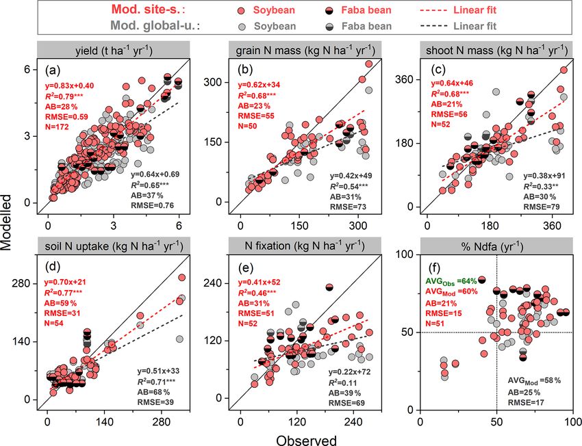
served variables, the coefficient of determination (adjusted yields generally agreed well with observations, especially in
R 2 ), relative bias (RB, Eq. 16), absolute bias (AB, Eq. 17), the site-specific simulation setup. These had a higher regres-
and the root mean square error (RMSE, Eq. 18) were com- sion slope (0.83) and lower absolute bias (28 %) compared
puted: with the global uniform simulation setup (Fig. 4a). N con-
Mi − Oi tent in grains and shoots showed lower agreement, with sim-
RB = × 100 %, (16)
Oi ulated values underestimating the observations for most sites
|Mi − Oi | (Fig. 4b–c), likely arising from two important N sources to
AB = × 100 %, (17) grain legumes not being captured well by the model (i.e., soil
Oi
v
u n N uptake and BNF, shown in Fig. 4d–e). The global uniform
u1 X run did not capture observed N fixation well, with a regres-
RMSE = t (Mi − Oi )2 , (18)
n i=1 sion slope of 0.22 and absolute bias of 39 %. The simulated
BNF compared to observations was notably improved when
where Mi and Oi indicate modeled and observed values, and using site-specific parameters, with the regression slope in-
n is the number of observations. To evaluate the fit of the in- creasing to 0.41 and the absolute bias being reduced to 31 %
terannual variability of modeled and reported yields on the (Fig. 4e). The field-based measurements showed that the N
country level, the standard deviation (SD) and Pearson cor- derived from the atmosphere (%Ndfa) was the main contrib-
relation coefficient (r, Eq. 19) were calculated: utor to the legumes’ total N uptake, ranging from 15 % to
Pn 95 %, with a mean of 64 % across all field trials. LPJ-GUESS
i=1 Mi − M Oi − O
r=q 2 Pn 2 , (19) generally captured the mean response well, with simulated
Pn
i=1 M i − M i=1 Oi − O %Ndfa being 60 % and 58 % in the site-specific and global
https://doi.org/10.5194/gmd-15-815-2022 Geosci. Model Dev., 15, 815–839, 2022
824                                                               J. Ma et al.: Modeling biological N fixation with LPJ-GUESS

uniform runs, respectively, despite several extreme disagree-         served increase in shoot and leaf biomass due to water sup-
ments at several faba bean sites (Fig. 4f).                           ply was 19 % and 21 %, respectively. In comparison, the site-
   A linear relationship between legume yields and the rate           specific parameterized model resulted in increases of 13 %
of BNF was found across a range of field sites in this study          and 14 %, respectively (15 % and 14 % for the global uni-
(Fig. S5a). Simulations from LPJ-GUESS mostly captured                form parameter run, see Fig. 5b). Overall, the observed soy-
the close correlation between these variables, with R 2 rang-         bean tissue biomass and N content under rain-fed and irri-
ing 0.46–0.63 (p < 0.001) in both runs, which is not far from         gated conditions, as well as their response to irrigation man-
the measured value of 0.67 (Fig. S5a). Linear regression pa-          agement, were captured reasonably well by the model at the
rameters (i.e., slope and intercept) in both runs were close to       US Florida site, despite some deviations from observations
the observations, indicating that the model reproduces the N          in some cases.
fixation effect on yield well for individual sites.
   A negative exponential relationship was observed be-               3.1.3   Response to nodulating soybean
tween N fertilizer application rate and N fixation across the
field trials (Fig. S5b). LPJ-GUESS reasonably reproduced              In Zapata et al. (1987), two field trials with non-nodulating
the decreased trend of BNF to N fertilizer increase, with             and nodulating soybean were conducted in Seibersdorf, Aus-
similar fitting functions to observations, although higher N          tria (16.5◦ E, 48.0◦ N; see Table S2), resulting in different
fixation rates were modeled in the highest-fertilized trial           plant C and N production at various growth stages. As de-
(600 kg N ha−1 ) compared with measurements (Fig. S5b).               scribed in Sect. 2.3, the nodulation process of legumes has
                                                                      not yet been implemented in LPJ-GUESS; we thus switched
3.1.2   Response to irrigation                                        off (on) the BNF function in the model to simply represent
                                                                      the non-nodulating (nodulating) soybean experiment.
The ability of the model to simulate the observed response of            During the growing season, yield and grain N mass in the
soybean tissue biomass and N mass to irrigation management            field trials increased rapidly after the vegetative stage, peak-
was examined using data from an experiment with rain-fed              ing around harvest. Simulations from LPJ-GUESS mostly
and irrigated treatments in Florida, USA (82.4◦ W, 29.6◦ N;           captured those seasonal dynamics and the response to nodu-
see Table S2). Since the timing and quantity of irrigation            lating soybean (Fig. 6a–b): the modeled increase in yield and
were not reported in the literature (DeVries et al., 1989a, b),       grain N mass due to nodulation was 34 % and 51 % in the
we assumed that soybean was irrigated automatically when              site-specific run (34 % and 45 % in the global uniform run),
it experienced water stress in the model, with the amount of          respectively, in line with the observed response of 20 % and
plant water deficit as supplemental irrigation.                       41 % at harvest (Table 2), which suggests appropriate sensi-
   The mean observed grain yields at harvest were 2.0 and             tivity of yield and N content in grain to N addition from N
2.9 t ha−1 under rain-fed and irrigated conditions, respec-           fixation. Similarly, the model generally reproduced the ob-
tively, whereas the modeled yields were 1.9 and 2.5 t ha−1            served seasonal pattern of shoot N mass well, but with some
for the site-specific parameter run and 1.6 and 2.1 t ha−1 for        underestimations in the nodulation trial (Fig. 6c).
the global uniform parameter run, suggesting good model                  Accumulated soil N uptake was captured reasonably well
performance for rain-fed crops but an underestimation of              over the entire growing season, with higher accuracy at har-
the effect of irrigation on yields (Fig. 5a). Grain dry mat-          vest in the global uniform simulation (Fig. 6d). Measured
ter over the cropping season was simulated to increase by             mineral N uptake from soils declined on average by 25 % in
32 % and 45 % on average in response to irrigation in the             response to nodulation. In comparison, the simulated reduc-
site-specific and global uniform runs, respectively. The ob-          tion in uptake was 50 % and 46 % for the site-specific and
servations show a similar response but with a higher increase         global uniform runs (Table 2). The BNF rates were low at
of 75 %. The modeled increase in grain N content caused by            the early growth stages when nodules were still establishing
irrigation also showed good agreement, with an increase of            and increased rapidly between floral initiation and the early
35 %–58 % in both runs, in line with the observed response            seed-filling, after which nodule senescence occurred and the
of 42 % (Fig. 5b).                                                    increase in N fixation rate declined until physiological ma-
   The model generally reproduced observed leaf biomass               turity (Fig. 6e). Simulations from LPJ-GUESS reproduced
and N mass better than the total aboveground production un-           the seasonal pattern of N fixation with some overestimations
der rain-fed and irrigated treatments, with higher accuracy in        in the accumulated BNF at the end of the growth period;
the site-specific run. Over the growing season there was an           the site-specific and global uniform runs simulated 113 and
obvious underestimation of the total aboveground produc-              140 kg N ha−1 , respectively, compared to the measured value
tion of biomass for both runs (Fig. 5a). This may be par-             of 103 kg N ha−1 (Table 2).
tially due to the fact that LPJ-GUESS at this point does not
model soybean hulls, which account for ∼ 15 %–20 % of the
total aboveground dry matter at harvest in the US soybean
rain-fed cropping system (Córdova et al., 2020). The ob-

Geosci. Model Dev., 15, 815–839, 2022                                                   https://doi.org/10.5194/gmd-15-815-2022
J. Ma et al.: Modeling biological N fixation with LPJ-GUESS 825
Figure 4. Comparison of modeled and observed yield (a), grain N mass (b), shoot N mass (c), soil N uptake (d), BNF (e), and %Ndfa (the
proportion of plant N derived from the atmosphere) (f) at harvest across all soybean and faba bean sites. Filled red and grey circles depict
the “site-specific” and “global uniform” runs, respectively. The dashed line is a fitted linear regression with red for site-specific and grey
for global uniform; ∗∗∗ and ∗∗ denote regressions statistically significant at p = 0.001 and 0.01, respectively; AB is absolute bias (Eq. 17),
represented in percent (%); the unit of RMSE is the same as the associated variable; AVG in (f) is the averaged value of %Ndfa across all
field trials.
Table 2. Comparison of modeled and observed yield (t ha−1 ), grain N mass (kg N ha−1 ), shoot N mass (kg N ha−1 ), soil N uptake
(kg N ha−1 ), and N fixation rate (kg N ha−1 ) from a soybean nodulation and non-nodulation experiment at harvest. The observed data were
compiled using Tables 2–4 in Zapata et al. (1987).
Nodulation Non-nodulation Nodulation effect (%)
Obs. Mod. site-s. Mod. global-u. Obs. Mod. site-s. Mod. global-u. Obs. Mod. site-s. Mod. global-u.
Yield 3.01 3.24 3.06 2.42 2.41 2.29 20 34 34
Grain N mass 162 166 148 115 110 102 41 51 45
Shoot N mass 222 198 181 158 134 138 41 48 31
Soil N uptake 119 76 86 158 152 159 −25 −50 −46
N fixation 103 140 113 – – – – – –
3.1.4 Response to N fertilizer in faba bean broadly reproduced these seasonal patterns and the response
to different N application rates. The largest difference be-
In the N fertilizer experiment from Mínguez et al. (1993), tween modeled and measured leaf biomass was found at
four field trials were compared with N applications between the end of the growing season as a result of the simulated
0 and 300 kg N ha−1 at three crop growth stages and two leaf senescence rate being much lower than derived from
faba bean varieties grown in a Mediterranean climate (Spain, measurements (Fig. 7a). In addition, the simulations showed
4.8◦ W, 37.9◦ N; see Table S2). Over the entire growing sea- modeled leaf N mass to decline rapidly during the late re-
son, leaf biomass and N content in the field trials increased productive phase. This can be attributed to the transfer of N
until around May, after which leaf senescence started and from vegetative parts to grain because of the high N demand
biomass and N content declined (Fig. 7a–b). The model in seeds during the grain-filling period.
https://doi.org/10.5194/gmd-15-815-2022 Geosci. Model Dev., 15, 815–839, 2022826 J. Ma et al.: Modeling biological N fixation with LPJ-GUESS
Figure 5. Comparison of modeled and observed soybean tissue biomass and N mass (a) and their responses to irrigation management (b)
compared with those grown at rain-fed conditions. Red and grey circles depict “site-specific” and “global uniform” run, respectively; the
dashed line is fitted linear regression; ∗∗∗ denotes the regression statistically significant at p = 0.001. Box plots in (b) denote the 5th and
95th percentiles with whiskers, median and interquartile range with box lines, and mean with a white dot (all data distributed next to the box).
The seasonal data at each phenological stage for tissue biomass are available from 1978–1979 and 1984–1985 with rain-fed and irrigated
treatments; those for N mass are available for 1979 and 1984, while the seasonal shoot N mass is only available for 1984.
As seen in Fig. 7c, modeled soil N uptake was stimulated 3.2 Model evaluation at global scale
by soil mineral N availability, with an increase of 120 %–
160 % compared to the unfertilized treatment. In contrast, 3.2.1 Attained yields
fixing N from the atmosphere was constrained in the pres-
ence of elevated levels of soil mineral N, with a reduction Using the global uniform parameters described in Sect. 2.4.1,
of 15 %–20 %. The total N uptake for the cropping season combined with the time-dependent gridded N fertilizer
1987–1988 was observed to only increase by 3 % in response dataset introduced in Sect. 2.4.2, we simulated soybean and
to N application as a consequence of the inoculation imple- all pulses (applying the faba bean parameterization, see
mented in the unfertilized treatment (Mínguez et al., 1993). Sect. 2.4.2) at a global scale. We computed data for the pe-
By contrast, LPJ-GUESS produced relatively large increases riod 1996–2005, since crop-specific fractional cover from the
of 14 %–16 % in both runs, resulting in the observed increase MIRCA dataset was available for the year 2000 (Portmann et
in plant biomass and N mass accumulation caused by N ad- al., 2010).
dition being largely overestimated in the model (Fig. 7c). Modeled yields in the top 10 soybean-producing coun-
tries showed good agreement, with a higher R 2 of 0.52
(p < 0.001) and lower RMSE value of 0.8 t ha−1 yr−1 when
low-productivity countries (defined as all countries not be-
longing to the top 10 producer countries) were excluded.
With all producer countries included, R 2 of 0.17 (p < 0.001)
Geosci. Model Dev., 15, 815–839, 2022 https://doi.org/10.5194/gmd-15-815-2022J. Ma et al.: Modeling biological N fixation with LPJ-GUESS 827
which grow under a broad range of climate and soil condi-
tions.
A good fit of the interannual variability of modeled and re-
ported yields is a further indicator of model performance. De-
spite the deviation between the model and observations for
individual years, simulated variation in soybean yield over
the period 1981–2016 matched reported yields well among
the top 10 producer countries – especially in Argentina, In-
dia, and China – with a high Pearson correlation coefficient
(r) around 0.60 (p < 0.001) and similar standard deviations
(Fig. 9). The degree of yield variability between years was
larger than seen in the FAO records, especially in the US,
Canada, and Italy (Fig. 9), indicating high sensitivity of mod-
eled soybean yield to changing environmental factors on spa-
tial scales, such as weather, N fertilizer application rates, and
climate-related N fixation.
3.2.2 N fixation and %Ndfa
The modeled spatial pattern of soybean N fixation showed
large spatial variation (Fig. 10a). Modeled BNF rates as high
as 250 kg N ha−1 yr−1 were found in western South America
and most of Africa, where neither water nor temperature was
a critical limitation for N fixation. Moreover, the relatively
low fertilizer application in Africa (0–20 kg N ha−1 yr−1 ,
Fig. S4b) leaves a nitrogen deficit that causes enhanced soy-
bean N fixation. In contrast, in arid and semi-arid regions,
soil water constrains BNF, while temperature limitation is
Figure 6. Observed (circles) and modeled (lines) yield (a), grain N seen in high latitudes and alpine areas (e.g., Andes in Peru).
mass (b), shoot N mass (c), soil N uptake (d), and BNF (e) for a field BNF rates in most regions (South Asia, West Asia, sub-
site in Austria (Zapata et al., 1987) for the cropping season 1984 Saharan Africa, and northwestern China) were as low as
with nodulating and non-nodulating soybean. The observed values 50 kg N ha−1 yr−1 , particularly in Pakistan and northern In-
of soil N uptake and BNF across all growth stages were calculated dia, where simulated BNF is severely constrained by the ex-
based on Fig. 1 given in Zapata et al. (1987), and the vertical bars treme high temperature over the cropping season. The eastern
represent the standard error of a four-replicate mean in the origi- United States, Europe, southern China, and central-western
nal literature. Veg. and Rep. indicate vegetative and reproductive Brazil showed intermediate fixation rates, which were greater
growth phase, respectively. than 150 kg N ha−1 yr−1 . Overall, the spatial variation of the
modeled legume BNF rate reflects to a large degree the spa-
tial climate patterns, in addition to N fertilizer application.
The low modeled %Ndfa of 45±3 % in East Asia may reflect
and RMSE of 1.4 t ha−1 yr−1 were found (Fig. 8a). LPJ- high N uptake from soils in response to substantial fertilizer
GUESS generally tended to overestimate the reported yield investment in China (80–180 kg N ha−1 yr−1 , Fig. S4b) over
for most countries where soybean production is low (e.g., the past 40 years. In contrast, the modeled %Ndfa in Africa –
most African countries, see Fig. 9a), with a mean relative with lower N application rates – was as high as 70 ± 3 %, al-
bias in such countries of 81 % (Fig. 8a). Modeled low yields though still lower than the reported mean value of 77 % (Ta-
were found in some arid and semi-arid countries (e.g., Egypt, ble 3). The spatial response of N fixation rate to climate con-
Iran, and Turkey), with the underestimation spanning from straining factors (i.e., soil temperature and water) is shown
10 %–70 % (Fig. 9a). Overestimated yields were also found for pulses in Fig. S6.
when comparing simulated yields using the faba bean param- At a regional scale, the modeled outputs compare well
eterization against FAO-reported values for pulses in general, with N fixation rates from the literature (Fig. 10b–f, Ta-
with an overestimation also visible for some of the top pro- ble 3). For example, in South America and North America,
ducing countries (Fig. 8b). Likely, the higher yields simu- both major soybean-producing regions, simulated BNF rates
lated by LPJ-GUESS arise from the fairly high N fixation were 156 ± 14 and 127 ± 44 kg N ha−1 yr−1 over the period
capacity simulated with the faba bean parameterization (see 1981–2016, respectively, compared with literature-derived
Sect. 3.2.2) and the wide distribution of pulses worldwide, values of 136 and 144 kg N ha−1 yr−1 (Peoples et al., 2009).
https://doi.org/10.5194/gmd-15-815-2022 Geosci. Model Dev., 15, 815–839, 2022You can also read