Environmental drivers of circum-Antarctic glacier and ice shelf front retreat over the last two decades
←
→
Page content transcription
If your browser does not render page correctly, please read the page content below

The Cryosphere, 15, 2357–2381, 2021
https://doi.org/10.5194/tc-15-2357-2021
© Author(s) 2021. This work is distributed under
the Creative Commons Attribution 4.0 License.

Environmental drivers of circum-Antarctic glacier and ice shelf
front retreat over the last two decades
Celia A. Baumhoer1 , Andreas J. Dietz1 , Christof Kneisel2 , Heiko Paeth2 , and Claudia Kuenzer1,2
1 German    Remote Sensing Data Center (DFD), German Aerospace Center (DLR),
82234 Weßling, Germany
2 Institute of Geography and Geology, University of Würzburg, Am Hubland, 97074 Würzburg, Germany

Correspondence: Celia A. Baumhoer (celia.baumhoer@dlr.de)

Received: 6 August 2020 – Discussion started: 21 September 2020
Revised: 26 March 2021 – Accepted: 12 April 2021 – Published: 20 May 2021

Abstract. The safety band of Antarctica, consisting of float-         Deep Water that is driven by strengthening westerlies and to
ing glacier tongues and ice shelves, buttresses ice discharge         further assess surface hydrology processes such as meltwater
of the Antarctic Ice Sheet. Recent disintegration events of           ponding, runoff, and lake drainage.
ice shelves along with glacier retreat indicate a weakening
of this important safety band. Predicting calving front re-
treat is a real challenge due to complex ice dynamics in a
data-scarce environment that are unique for each ice shelf            1   Introduction
and glacier. We explore the extent to which easy-to-access
remote sensing and modeling data can help to define envi-             A safety band of floating ice shelves and glacier tongues
ronmental conditions leading to calving front retreat. For the        fringes the Antarctic Ice Sheet (AIS) (Fürst et al., 2016).
first time, we present a circum-Antarctic record of glacier           Large glacier tongues and ice shelves create buttressing ef-
and ice shelf front change over the last two decades in com-          fects, decreasing ice flow velocities and ice discharge (De
bination with environmental variables such as air tempera-            Rydt et al., 2015; Gagliardini et al., 2010; Royston and Gud-
ture, sea ice days, snowmelt, sea surface temperature, and            mundsson, 2016). The recent large-scale retreat of ice shelf
wind direction. We find that the Antarctic Ice Sheet area             and glacier fronts along the Antarctic Peninsula (AP) and the
decreased by −29 618 ± 1193 km2 in extent between 1997–               West Antarctic Ice Sheet (WAIS) indicates a weakening of
2008 and gained an area of 7108 ± 1029 km2 between 2009               this safety band (Rott et al., 2011; Rankl et al., 2017; Friedl
and 2018. Retreat concentrated along the Antarctic Penin-             et al., 2018; Cook and Vaughan, 2010). Calving front re-
sula and West Antarctica including the biggest ice shelves            treat can increase ice discharge and hence the contribution
(Ross and Ronne). In several cases, glacier and ice shelf re-         to global sea level rise (De Angelis and Skvarca, 2003; See-
treat occurred in conjunction with one or several changes             haus et al., 2015). Increases in ice discharge occur if ice
in environmental variables. Decreasing sea ice days, intense          shelf areas with strong buttressing forces are lost (Fürst et al.,
snowmelt, weakening easterlies, and relative changes in sea           2016). The current contribution of the Antarctic Ice Sheet to
surface temperature were identified as enabling factors for           global sea level rise is 7.6 ± 3.9 mm (1992–2017), but over
retreat. In contrast, relative increases in mean air tempera-         this study period a strong trend of mass loss acceleration was
ture did not correlate with calving front retreat. For future         observed for West Antarctica after ice shelves and glaciers
studies a more appropriate measure for atmospheric forcing            retreated and thinned (IMBIE, 2018). In contrast, there is no
should be considered, including above-zero-degree days and            clear trend in the mass balance of the East Antarctic Ice Sheet
temperature extreme events. To better understand drivers of           (EAIS). Since the 1990s altimetry measurements have shown
glacier and ice shelf retreat, it is critical to analyze the magni-   a small gain (but with high uncertainties) for the EAIS, with
tude of basal melt through the intrusion of warm Circumpolar          5 ± 46 Gt/yr (1992–2017) (IMBIE, 2018). However, a strong
                                                                      mass loss trend of −47 ± 13 Gt/yr (1989–2017) is calculated

Published by Copernicus Publications on behalf of the European Geosciences Union.
2358                                             C. A. Baumhoer et al.: Circum-Antarctic glacier and ice shelf front retreat

using the mass budget method (Rignot et al., 2019). Glacier        hydrofracture (Kopp et al., 2017; Pollard et al., 2015), lake
terminus positions along the EAIS experienced a phase of           ponding, and lake drainage (Banwell et al., 2013; Leeson et
retreat between 1974 and 1990 followed by a phase of ad-           al., 2020). Ocean forcing weakens the floating ice as a result
vance until 2012. The single exception to this advance in East     of basal melt inducing thinning and grounding line retreat
Antarctica is Wilkes Land, where retreating glacier fronts         (Konrad et al., 2018; Paolo et al., 2015; Rignot et al., 2013)
were observed (Miles et al., 2016).                                as well as by warmer ocean surface water undercutting the
   The coastline of the Antarctic Ice Sheet is defined as the      ice cliff at the waterline (Benn et al., 2007) by reducing sta-
border between the ice sheet and the ocean (Liu and Jezek,         bilizing fast ice (Larour, 2004) and through enhanced sea ice
2004), extending along glacier and ice shelf fronts. Through-      reduction (Massom et al., 2018; Miles et al., 2016). Environ-
out this paper, we refer to floating glacier tongues and ice       mental forcing on tidewater glaciers has been frequently ob-
shelves when using the term “glacier and ice shelf front” as       served on Greenlandic glaciers (Cowton et al., 2018; Howat
well as “calving front”. Whether a glacier or ice shelf front      et al., 2008; Luckman et al., 2015), but for Antarctica in
advances or retreats depends mainly on four different factors:     many regions it is unclear where and at what amount envi-
internal ice dynamics, geometry, external mechanical forc-         ronmental drivers cause calving front retreat (Baumhoer et
ing, and external environmental forcing (Alley et al., 2008;       al., 2018; Pattyn et al., 2018).
Benn et al., 2007; Cook et al., 2016; Luckman et al., 2015;           Current knowledge on environmentally forced calving
Walker et al., 2013). The combined influence of those factors      front retreat in Antarctica can be summarized by the follow-
make it challenging to create a realistic calving law, making      ing studies.
iceberg calving still one of the least understood ice shelf pro-      Glacier retreat along the Antarctic Peninsula was first only
cesses (Bassis, 2011). Frontal retreat starts with the forma-      associated with atmospheric warming (Cook et al., 2016;
tion of a crevasse originating from a strain rate surpassing the   Mercer, 1978) until more recent studies identified ocean forc-
yield stress of ice (Mosbeux et al., 2020). For ice shelves and    ing as the main driver (Cook et al., 2016; Wouters et al.,
floating glacier tongues, the calving position evolves where       2015). Additionally, the formation of melt ponds on the
crevasses develop into through-cutting fractures (rifts). These    ice shelf surface has been discussed as an enhancing fac-
ice shelf rifts can propagate further into the ice front or in-    tor for calving. Meltwater can initiate crevasse propagation,
tersect with other rifts, resulting in a tabular iceberg calv-     resulting in hydrofracture and ice shelf retreat (Scambos et
ing event (Benn et al., 2007; Joughin and MacAyeal, 2005),         al., 2000; Scambos et al., 2017). The poleward shift in the
where the extent of the ice shelf and the size of the iceberg      west wind drift causes upwelling Circumpolar Deep Water
are defined by the rift location (Lipovsky, 2020; Mosbeux          (CDW). This allows warmer ocean waters to reach the bot-
et al., 2020; Walker et al., 2013). Further boundary condi-        tom of ice shelves, inducing basal melt and ice shelf thin-
tions such as fjord geometry (Alley et al., 2008; Catania et       ning, as observed in the Bellingshausen and Amundsen sea
al., 2018), ice rises and rumples (Matsuoka et al., 2015), and     sectors (Dutrieux et al., 2014; Thoma et al., 2008; Wouters et
bed topography (Hughes, 1981) influence the stability of the       al., 2015). Basal melt, when combined with a retrograde bed
calving margin.                                                    (Scheuchl et al., 2016; Hughes, 1981), has led to a retreat of
   The previously described natural cycle of growth and de-        the grounding line followed by increased ice discharge (Kon-
cay of a glacier or ice shelf (Hogg and Gudmundsson, 2017)         rad et al., 2018; Rignot et al., 2013), for example at the for-
can be disturbed by external mechanical and environmental          mer Wordie Ice Shelf (AP) (Friedl et al., 2018; Walker and
forces. It was found that mechanical forcing arises from tides     Gardner, 2017). In contrast, the retreat of calving fronts along
(Rosier et al., 2014), ocean swell (Massom et al., 2018), ice-     Wilkes Land (EAIS) has been associated with a reduction in
berg collision (Massom et al., 2015) and tsunamis (Walker          the duration of the sea ice cover (Miles et al., 2016).
et al., 2013), which can destabilize floating ice shelves and         The drivers of ice shelf and glacier retreat and advance
glacier tongues initiating iceberg calving (Alley et al., 2008).   can be manifold depending on studied variables, time pe-
Glaciers and ice shelves are in direct interaction with the at-    riods, and regions. Therefore, the identification of environ-
mosphere and ocean and are hence sensitive to changes in           mental driving forces for fluctuations in ice shelf and glacier
environmental conditions (Vaughan and Doake, 1996; Kim             extent is challenging and has been the subject of many dis-
et al., 2001; Domack et al., 2005; Wouters et al., 2015).          cussions in the past. So far, there has not been a compre-
Environmental drivers can destabilize floating ice tongues         hensive analysis comparing circum-Antarctic glacier termi-
and shelves through various oceanically and atmospherically        nus change on a continental scale within uniform timescales
forced processes, causing mechanical weakening and frac-           (Baumhoer et al., 2018). In this paper, we explore Antarctic
turing (Pattyn et al., 2018). Instead of sporadic calving by       calving front change over the last two decades by analyzing
tabular icebergs (a sign of a natural calving event within         Antarctic coastal change (see Fig. 1) and address the ques-
the calving cycle), more frequent small-scale calving events       tion of whether or not environmental drivers forced the ob-
can occur as a result of environmental forcing (Liu et al.,        served changes in glacier and ice shelf front fluctuations. We
2015). Destabilization through atmospheric forcing arises          compare changes in Antarctic calving fronts in two decadal
from thinning through surface melt (Howat et al., 2008),           time steps (1997–2008 and 2009–2018) to minimize the ef-

The Cryosphere, 15, 2357–2381, 2021                                                   https://doi.org/10.5194/tc-15-2357-2021

C. A. Baumhoer et al.: Circum-Antarctic glacier and ice shelf front retreat                                                   2359

fect of short-term glacier front fluctuations. To identify po-    ing in situ observations to modeled data prove that ERA5
tential links between calving front retreat and recent changes    surface air temperature (2 m temperature) outperforms the
in the Antarctic environmental conditions, we correlated two      former ERA-Interim product. ERA5 temperature data have
decades of glacier change with climate data, including air and    the ability to capture annual variability and the magnitude of
sea surface temperature as well as changes in wind direction,     temperature change over the Antarctic Ice Sheet (Tetzner et
snowmelt, and sea ice cover.                                      al., 2019; Gossart et al., 2019). The mean absolute error is
                                                                  2.0 ◦ C, with higher accuracies in the coastal areas and less
                                                                  accurate results in the interior of the ice sheet (Gossart et al.,
2     Processed and analyzed data sets                            2019). Tetzner et al. (2019) reports much higher accuracies
                                                                  for the Antarctic Peninsula, with a mean absolute error of
2.1    Coastlines
                                                                  −0.13 ◦ C. Compared to the mean, the variability in tempera-
To calculate the decadal retreat and advance of Antarctic         ture is captured with high accuracy at a mean Pearson corre-
glaciers and ice shelves, we use calving front positions of       lation coefficient of 0.98 (Gossart et al., 2019; Tetzner et al.,
three Antarctic coastline products from 1997, 2009, and           2019). We divided temperature measurements into the cooler
2018. Timewise, we refer to first (1997–2008) and sec-            half (“winter”: April–September) of the year and warmer half
ond (2009–2018) decade even though the time periods are           (“summer”: October–March) to separate the environmental
11 and 9 years, respectively, limited by the availability of      forcing for different seasons.
coastline products. The first coastline product was automat-         Snowmelt data should be handled with care as accuracy as-
ically extracted from the high-resolution Radarsat-1 mo-          sessments for the ERA5-Land snowmelt product were not yet
saic by adaptive thresholding and finalized by manual cor-        performed. Surface mass balance (SMB) data including mod-
rection (Liu and Jezek, 2004). The Radarsat-1 mosaic im-          eled snowmelt data were found to slightly underestimate the
agery was acquired between September and October 1997             SMB (Gossart et al., 2019). Snowmelt is calculated within
with a spatial resolution of 25 m. The entire data set is         the summer months December, January, and February, when
freely available at the National Snow and Ice Data Cen-           most melt occurs. The amount of snowmelt is calculated in
ter (NSIDC) at https://nsidc.org/data/NSIDC-0103/versions/        millimeters of water equivalent (mm w.e.) per day.
2 (last access: 25 February 2020) (Jezek et al., 2013). Glacier      The Antarctic continent is circled by weak and irregular
and ice shelf fronts for the year 2009 were manually de-          easterly winds driven by high-pressure areas over the inte-
lineated from the MOA 2009 surface morphology image               rior of the Antarctic continent created by cold and dry air.
map acquired during austral summer 2008/2009 (November–           Easterlies weaken in the case of a positive Southern An-
February) with a spatial resolution of 125 m (Scambos et          nular Mode (SAM) as the west wind drift shifts poleward.
al., 2007). This data set is also freely available at NSIDC       In order to assess those changes in wind direction, we use
from https://nsidc.org/data/NSIDC-0593/versions/1 (last ac-       ERA5 monthly averaged zonal (west to east) wind speed
cess: 25 February 2020) (Haran et al., 2014). The coast-          estimations at 10 m above the surface with a lateral resolu-
line for 2018 was automatically extracted via a fully con-        tion of approx. 31 km. ERA5 captures the spatial variability
volutional network from Sentinel-1 mid-resolution (40 m)          in near-surface wind speed but underestimates strong winds
dual-pol imagery (see Methods section). Directly calculat-        and coastal winds, whereas the wind speed over the inte-
ing coastal change between these coastline products includes      rior is captured very accurately during summer (Gossart et
changes in floating calving fronts and grounded ice walls (as     al., 2019). Over the ocean, ERA5 annual mean zonal wind
shown in Fig. 1) even though the amount of change from            speed is considerably underestimated compared to ASCAT
grounded termini is small and prone to inaccuracies due to        (Advanced Scatterometer) observations (Belmonte Rivas and
the low spatial resolution of the coastline product from 2009.    Stoffelen, 2019). Overall, the mean absolute error over the
                                                                  continent is 2.8 m/s, with high variance in space and time,
2.2    ERA5 reanalysis data                                       but an accurate representation of the annual variability in
                                                                  zonal wind speed is achieved (Gossart et al., 2019). ERA5
We use ERA5-Land monthly averaged atmospheric reanal-             monthly averaged data on single levels are freely available at
ysis data for air temperature and snowmelt information            the Copernicus Climate Change Service Climate Data Store
(Copernicus Climate Change Service, 2019b). It is the most        (CDS) (Copernicus Climate Change Service, 2019a). Zonal
state-of-the-art reanalysis product from the European Cen-        wind was calculated for the summer months (DJF) because
tre for Medium-Range Weather Forecasts (ECMWF), replac-           easterly winds show a weakening trend during summer but
ing the former ERA-Interim product (Hersbach et al., 2020).       not throughout the entire year (Hazel and Stewart, 2019).
Data are available from 1981/1982 to present day at a 9 km
spatial resolution. As ground-based meteorological observa-       2.3   Sea ice days
tions are scarce over the Antarctic continent, we decided to
use the reanalysis data even though modeled data are less         The most recent Global Sea Ice Concentration Climate Data
accurate compared to in situ measurements. Studies compar-        Record (Version 2) (Lavergne et al., 2019) was downloaded

https://doi.org/10.5194/tc-15-2357-2021                                                 The Cryosphere, 15, 2357–2381, 2021
2360                                                C. A. Baumhoer et al.: Circum-Antarctic glacier and ice shelf front retreat

Figure 1. Coastal change in Antarctica between 1997 and 2018 with enlarged views (counterclockwise) for Larsen C Ice Shelf, Pine Island
Bay, Oates Land, Wilkes Land, Shackleton Ice Shelf, Shirase Bay, and Dronning Maud Land. Colors indicate the timing of retreat and
advance. The pie chart visualizes losses and gains in the area of the Antarctic Ice Sheet with regard to the indicated year. Labels of coastal
sectors are shown in gray, seas in light blue, bays in dark blue, and ice shelves and glaciers in black and white fonts. Background: LIMA
Landsat Mosaic.

from the Ocean and Sea Ice Satellite Application Facility                ice extent is very similar between OSI and ice chart prod-
(OSI SAF, 2017). We used the daily product (OSI-450, OSI-                ucts (Brandt-Kreiner et al., 2019), which allows the assump-
430-b) during sea ice months April through October, in line              tion of a very accurate data set. The product has a resolu-
with previous studies (Massom et al., 2013; Miles et al.,                tion of 25 km × 25 km. In order to calculate actual sea ice
2016). The product covers the time period 1982 to 2018 and               days, we count each pixel per day with a sea ice concentra-
is derived from passive microwave data acquired by Nim-                  tion higher than 15 % as suggested by previous studies (Miles
bus 7 and Defense Meteorological Satellite Program (DMSP)                et al., 2016; Massom et al., 2013). During the early acquisi-
satellites. The final sea ice concentration is computed by the           tion years data gaps occur, and second-daily acquisitions ex-
passive microwave data in combination with ERA-Interim                   ist until mid 1987. In this case, we multiplied the monthly
data. The standard deviation of mismatch between OSI prod-               available sea ice days by the proportional number of missing
ucts and ice chart analysis on sea ice concentration is 8 %              days. We decided not to use data for the year 1986 as data for
for ice and open water during winter (JJA). The trend in sea

The Cryosphere, 15, 2357–2381, 2021                                                            https://doi.org/10.5194/tc-15-2357-2021

C. A. Baumhoer et al.: Circum-Antarctic glacier and ice shelf front retreat                                                 2361

entire months were missing, and mean sea ice days per year         mented tiles within one zone was calculated and then thresh-
could not be calculated accurately.                                olded by a prediction probability of 50 % for the class land
                                                                   ice. In case of multi-coverage by several satellite scenes,
2.4    Sea surface temperature                                     more robust results were obtained by merging the predic-
                                                                   tion probabilities. Morphological filtering and the exclusion
Sea surface temperature measured by satellite sensors is also      of higher ice sheet areas by integrating elevation information
provided by the CDS (Copernicus Climate Change Service,            from the TanDEM-X Polar DEM 90 (Wessel et al., 2021) re-
2019a). The most up-to-date product Level 4 (Version 2) con-       duced further errors. Finally, from the binary segmentation
sists of multiple satellite observations from the NOAA, ERS        results, the border between both classes was extracted as the
(European Remote Sensing Satellites), Envisat, and Sentinel-       final coastline.
3 satellites, with a 0.05◦ gridded resolution (approx. 5.5 km).
We calculated surface temperatures only for the months with        3.2   Derivation of calving front change
little to no sea ice cover (October–March). This reduces er-
rors over sea ice, where the thickness and concentration of        Calving front change was estimated by calculating the
sea ice can account for large measurement errors (Kwok and         change in area between the coastlines in 1997, 2009, and
Comiso, 2002). Uncertainties in Level 4 data vary depending        2018 over the area of floating glacier tongues and ice shelves
on the year of acquisition and latitude of measurement. The        excluding grounded glacier termini. As coastline extraction
median difference compared to in situ drifter measurements         and delineation are very subjective tasks, and all coastlines
is up to −0.4 ◦ C for low latitudes during the early acquisition   originated from different sources and resolutions, deviations
years before 1996. Afterwards the accuracy increases to bet-       occurred in many areas. Areas of fast ice, mélange, and ice-
ter than −0.1 ◦ C for low latitudes. A stability assessment of     bergs trapped in sea ice were error sources. For the automati-
the Level 4 product calculated a maximum trend of 0.01 ◦ C         cally extracted 2018 coastline, errors existed along the west-
per year (Embury, 2019). A summary of all processed climate        ern Antarctic Peninsula and in areas where only single-pol
variables is given in Table 1.                                     imagery was available. The MODIS-derived coastline often
                                                                   included snow-covered sea ice, which is difficult to distin-
                                                                   guish from glacier ice in optical imagery. To minimize errors
3     Methods                                                      and mismatches, all three coastlines were manually corrected
                                                                   and adjusted. Each coastline product was corrected based on
3.1    Extraction of Sentinel-1 coastline
                                                                   the satellite imagery from which they were originally cre-
We use a modified version of the automatic coastline extrac-       ated. After manual correction any change in area between the
tion approach published by Baumhoer et al. (2019) to ex-           coastline products could be attributed to glacier front change.
tract the Antarctic coastline for 2018. To cover the entire        From each coastline a raster (resolution 40 × 40 m) was cre-
Antarctic coastline, 158 dual-pol and 17 single-pol medium-        ated with a unique value over the ice-covered area. All three
resolution Sentinel-1 scenes were processed. Dual-polarized        raster layers were stacked and summed up, so each raster
scenes contain radar backscatter values for the polarizations      value pixel is associated with retreat or advance of the spe-
HH and HV, whereas single-polarized scenes only include            cific year. The area change was calculated for each major
the HH polarization. The coastline was split into 18 zones         floating ice shelf and glacier tongue wider than 3 km based
based on ice flow divides, defining major ice sheet basins af-     on a 40 m resolution raster in polar stereographic projec-
ter Rignot et al. (2011). For each zone all available scenes       tion. To account for inaccuracies in the manual adjustment of
acquired during winter months (June–August) in 2018 were           all coastlines, we measured the accuracy as the area change
selected. Depending on the scene availability, each zone was       over 30 randomly picked stable coastline areas. Any change
covered at least by one Sentinel-1 scene and in the best           over those regions can be attributed to errors in manual de-
case by three scenes. In case no dual-pol scenes were avail-       lineation, imagery resolution differences, and errors in or-
able, single-pol data were selected. First, each scene was         thorectification of the different satellite image mosaics. The
pre-processed (thermal correction, calibration, terrain correc-    error is calculated per kilometer of the coastline and calcu-
tion), masked with a coastline buffer of 100 km, and tiled         lated in proportion to the measured front length. On average,
into 780 × 780 pixel tiles. The convolutional neural network       the coastlines deviated ±1.2 pixels per kilometer per year.
(CNN) U-Net was used to segment each tile into the class           Broken down for each coastline product, the error between
ocean and the class land ice. We trained the U-Net on 15 dif-      1997–2009 was 0.4 pixels per kilometer per year, 2.3 pixels
ferent Antarctic coastal regions during various seasons with       per kilometer per year between 2009–2018, and 0.9 pixels
40 036 image tiles from 75 Sentinel-1 scenes. For single-pol       per kilometer per year between 1997–2018.
scenes we retrained our network for HH-polarized images
only. This decreased the accuracy slightly as only one po-
larization limits the information on surface backscatter char-
acteristics. In the post-processing step the mean of all seg-

https://doi.org/10.5194/tc-15-2357-2021                                                 The Cryosphere, 15, 2357–2381, 2021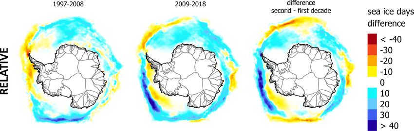
2362                                                 C. A. Baumhoer et al.: Circum-Antarctic glacier and ice shelf front retreat

Table 1. Summary of processed climate variable data sets.

   Climate                   Time           Season                           Spatial      Accuracy             Data                    Data
   variable                  span                                            resolution                                                store
   Air temperature           1982–2018      Summer (October–March)           9 km         0.13–2.0 ◦ C         Modeled                 CDS
                                            Winter (April–September)
   Snowmelt                  1982–2018      December–February                9 km         –                    Modeled                 CDS
   Zonal wind                1982–2018      December–February                31 km        2.8 m/s              Modeled                 CDS
   Sea ice days              1982–2018      April–October                    25 km        8 % standard devi-   Modeled + satellite     Osisaf
                             (not 1986)                                                   ation compared to
                                                                                          ice chart
   Sea surface temperature   1982–2018      October–March                    ∼ 5.5 km     −0.1 to −0.4 ◦ C     Multiple   satellites   CDS

3.3    Climate data correlation                                        basins with variable averages for the two different decades
                                                                       (1997–2008 and 2009–2018).
In order to assess the influence of climate variables (such
as air temperature, sea ice days, sea surface temperature,
snowmelt, and zonal wind) on glacier and ice shelf retreat,            4     Results
we spatially correlated the percentage of advance and re-
treat for each minor glacier basin (as defined by Mouginot,            4.1     Advance and retreat of Antarctic glaciers and ice
2017) with the decadal mean value of each climate variable.                    shelves
Means were calculated from 37 years of climate data for the
three time periods 1982–1996, 1997–2008, and 2009–2018.                Circum-Antarctic glacier and ice shelf front changes were
The first period is used as the reference period to measure            assessed by comparing Antarctic coastline products during
temporal changes in the following two decades. Hence, the              1997–2008 and 2009–2018. The results are shown in Fig. 2.
inputs of the correlation covered the two time spans 1997–             Between 1997 and 2008 ice shelf and glacier extents de-
2008 and 2009–2018 for which also the glacier retreat was              creased by −29 618 ± 1193 km2 , where 69 % of the total
calculated. To also assess relative changes in the variables           changed area retreated, and 31 % advanced (see Table 2 for
at previous times, we subtracted the reference mean (1982–             all change rates). In contrast, during the period 2009 to 2018
1996). This means the relative values indicate the change in           a slight area increase of 7108 ± 1029 km2 could be observed,
an environmental variable within the first and second decade           with 44 % of the total changed area retreating and 56 % ad-
compared to the reference time frame. Zonal wind, sea ice              vancing. The locations of area change are almost similar
coverage, and sea surface temperature means were calcu-                for both observation periods. Ice shelves along the Antarctic
lated within a 100 km seawards buffer along the coastline.             Peninsula retreated over the entire observation period (1997–
Mean air temperature and snowmelt were calculated within a             2018). The only exception was the advance of the Larsen D
100 km buffer landwards from the coastline, covering the sur-          Ice Shelf, which is located close to the Ronne Ice Shelf in the
face of ice shelves. The 100 km landwards buffer was chosen            Weddell Sea (see Fig. 2). Between 1997 and 2008, the large
as the best trade-off to calculate averages over the ice shelf         disintegration events of the Larsen B, Wilkins, and Wordie
area by not including too much of the ice sheet. Due to a              ice shelves resulted in a 37 % higher calving amount from the
circum-Antarctic analysis, this is only a rough approxima-             Antarctic Peninsula as compared to the amount calved from
tion, and especially over smaller glaciers within steep terrain,       this region between 2009–2018. During the second decade
the average includes changes not only over the glacier tongue          the breakup of iceberg A-68 from the Larsen C Ice Shelf and
but also the surrounding area. Again, relative values were cal-        the further disintegration of the Wilkins Ice Shelf were re-
culated by subtracting the reference mean 1982–1996. To re-            gions of strong area loss. In total, the rate of retreat along
move the effect of different basin sizes and different amounts         the Antarctic Peninsula was 5–6 times higher than glacier
of ice discharge, we took the percentage of advance and re-            advance in this region over the last 20 years.
treat within each basin instead of the absolute value for the             West Antarctica lost more than 3 times as much calving
correlation. Input data for the Pearson correlation were the           area in the first decade (1997–2008) compared to 2009–2018.
mean of all assessed climate variables (absolute and relative          In West Antarctica, 75 % of glacier and ice shelf retreat can
averages) as well as the percentage of retreat and advance.            be attributed to the calving of Ronne and Ross West ice
This created 14 different variables, which were correlated             shelves during the first decade. The retreat at WAIS was sig-
with each other based on 188 observations (N = 188). The               nificantly lower in the second decade, whereas the Ross and
number of observations is derived from 94 assessed glacier             Ronne ice shelves started to advance again. Excluding these

The Cryosphere, 15, 2357–2381, 2021                                                            https://doi.org/10.5194/tc-15-2357-2021
C. A. Baumhoer et al.: Circum-Antarctic glacier and ice shelf front retreat                                                   2363

two ice shelves, the rest of West Antarctica experienced pre-       the difference in the number of sea ice days per year (dur-
dominant glacier and ice shelf retreat during both observa-         ing the sea ice season April–October) compared to the ref-
tion periods as shown in Fig. 2. Pine Island and Thwaites           erence mean. The strongest decrease in sea ice days could
glaciers retreated over the entire observation period (1997–        be observed at the northern tip of the Antarctic Peninsula,
2018). The Getz and Abbot ice shelves had stable front posi-        with a shorter sea ice cover per year by up to 40 d during the
tions in the first decade but started to retreat after 2008. Only   first decade compared to the reference mean. During 1997
the Crosson Ice Shelf showed a contradicting pattern, with          and 2008 a decrease in sea ice days was observed along the
retreat in the first and re-advance in the second decade.           Bellingshausen Sea Sector, with up to 20 d less, and in the
   The glaciers and ice shelves of the EAIS showed an               Amundsen Sea Sector, with up to 5–10 d less. Compared to
overall stable advancing tendency with similar rates for            the first decade, the mean sea ice cover persisted longer in the
both decades, with 2638 ± 418 km2 more retreat during the           second decade along the Antarctic Peninsula and the Belling-
first (attributed to calving of Ross East Ice Shelf) and no         shausen Sea Sector, whereas in the Amundsen Sea Sector
clear change in advance (104 ± 872 km2 ) during the second          the sea ice days decreased by up to 10 d less compared to
decade. The strongest advance was observed for the Amery            the first decade. Along East Antarctica, sea ice coverage in-
and Filchner ice shelves as well as at the shelves of Dron-         creased 10 d on average except for Dronning Maud Land,
ning Maud Land and Queen Mary Land (see Fig. 1 for lo-              with a slight decrease of up to 5 d. When comparing the
cation). During 1997–2008, clear retreat appeared for the           two decades more sea ice days occurred during 2009 to 2018
Ross East Ice Shelf and along Enderby Land, especially in           along East Antarctica and the northernmost Antarctic Penin-
Shirase Bay. Wilkes Land and Victoria Land shared equal             sula, whereas the decrease along West Antarctica continues.
proportional amounts of retreat and advance. Between 2009           Changes in sea ice days were less extreme along East Antarc-
and 2018, the Ross Ice Shelf and Enderby Land entered a             tica, with ±10 d in difference compared to 1982–1996. Be-
phase of advance whereas Wilkes Land, George V Land, and            tween 1997–2008 the duration of sea ice cover was up to 5 d
Adélie Land started to retreat predominately.                       shorter along Dronning Maud Land and Wilkes Land com-
                                                                    pared to the reference mean. In the second decade sea ice
4.2   Air temperature                                               days along all of East Antarctica increased, with the high-
                                                                    est increase along Wilkes Land, by up to 10 d (compared to
The mean Antarctic air temperature was equal for both               1982–1996).
decades during winter but in summer +0.6 ◦ C higher in the
second decade (2009–2018). However, the overall mean does           4.4   Sea surface temperature
not reflect the strong regional differences in air tempera-
ture changes as shown in Fig. 3. During summer and win-             The changes in sea surface temperature during months with
ter the Antarctic Peninsula and the adjoining coast along           little sea ice cover (October–March) relative to the refer-
the Bellingshausen and Amundsen sea sectors as well as              ence mean are shown in Fig. 5 (absolute values in Fig. S2).
Queen Mary Land (EAIS) were cooler between 2009–2018,               Sea surface temperatures of the Southern Ocean cooled
whereas the interior of the ice sheet warmed during this pe-        (∼ −0.5 ◦ C) along East Antarctica and warmed along West
riod. Compared to the reference mean (1982–1996) summer             Antarctica and the western Antarctic Peninsula (∼ +0.5 ◦ C)
temperatures between 1997–2008 were cooler except for the           within the last two decades compared to 1982–1996, which
Peninsula, Queen Mary Land, and the Ross West and Filch-            is above the data uncertainty of 0.1 to 0.4 ◦ C. The warming
ner ice shelves. In the second decade this changed in sign          was less strong in the first decade and intensified within the
where the Antarctic Peninsula started to cool down and the          second decade, especially in the Bellingshausen Sea Sector,
interior increased in temperature. For the winter months al-        with maxima at George VI north (+0.65 ◦ C) and Pine Island
most over the entire Antarctica continent a warming ten-            Bay (+0.35 ◦ C) and with a slightly weaker increase along
dency was observed compared to the reference mean. The              the Amundsen Sea Sector (+0.15 ◦ C). The cooling along the
only exceptions were Victoria Land, Oates Land, and George          East Antarctic was less strong in the second decade. Along
V Land (all EAIS). Additionally, over the Getz Ice Shelf            East Antarctica for Amery Ice Shelf (+0.35 ◦ C), West Ice
(WAIS) cooler temperatures by 1 ◦ C occurred in 2009–2018           Shelf (+0.2 ◦ C), and Shackleton Ice Shelf (+0.25 ◦ C) warm-
compared to the reference mean. For Dronning Maud Land              ing was observed compared to the first decade.
(EAIS) a strong change was observed as the ice shelf surfaces
warmed up to 1.8 ◦ C in the second decade.                          4.5   Snowmelt

4.3   Sea ice days                                                  Snowmelt over the Antarctic Peninsula (see Fig. 6) was more
                                                                    extensive during the reference mean compared to the recent
Changes in sea ice days are shown in Fig. 4, and absolute           two decades. This is the reason why relative snowmelt in
numbers for sea ice days are provided in the Supplement             1997–2008 and 2009–2018 was mostly negative, with up to
in Fig. S1. A decrease or increase in sea ice days refers to        −0.3 mm w.e. per day. Nevertheless, strong snowmelt also

https://doi.org/10.5194/tc-15-2357-2021                                                  The Cryosphere, 15, 2357–2381, 2021
2364                                                C. A. Baumhoer et al.: Circum-Antarctic glacier and ice shelf front retreat

Table 2. Retreat and advance rates of Antarctic glaciers and ice shelves for each basin between 1997 and 2018 (upper table). Total lost and
gained ice shelf or glacier area per decade (lower table). For basin abbreviations see Fig. 2.

                                  1997–2008                               2009–2018                                1997–2018
           Basin     Advance (km2 /yr)   Retreat (km2 /yr)    Advance (km2 /yr)    Retreat (km2 /yr)   Advance (km2 /yr)   Retreat (km2 /yr)
   EAIS    A-Ap             249 ± 14.9          164 ± 17.4          295 ± 27.5             112 ± 13          215 ± 11.8             85 ± 6.5
           Ap-B               62 ± 4.8            89 ± 5.6            80 ± 8.9             53 ± 4.2            34 ± 3.8             36 ± 2.1
           B-C               187 ± 1.9              4 ± 2.2          186 ± 3.5             20 ± 1.6           179 ± 1.5              4 ± 0.8
           C-Cp              380 ± 7.7             167 ± 9          363 ± 14.2            153 ± 6.7           323 ± 6.1            111 ± 3.3
           Cp-D               49 ± 4.6            58 ± 5.4            45 ± 8.6             97 ± 4.1            23 ± 3.7               51 ± 2
           D-Dp                154 ± 5            64 ± 5.8           156 ± 9.2            317 ± 4.3            85 ± 3.9            111 ± 2.2
           Dp-E               68 ± 9.5           58 ± 11.1           74 ± 17.5              81 ± 8.3           34 ± 7.5             32 ± 4.1
           E-Ep                  6±3             411 ± 3.5           156 ± 5.5               8 ± 2.6            5 ± 2.4            154 ± 1.3
           Jpp-K             163 ± 2.1              2 ± 2.4          252 ± 3.8               2 ± 1.8          203 ± 1.6              1 ± 0.9
           K-A               306 ± 7.8            23 ± 9.1          285 ± 14.3              82 ± 6.8          270 ± 6.2             24 ± 3.4
           EAIS            1626 ± 61.1        1040 ± 71.4         1894 ± 112.9          926 ± 53.4          1370 ± 48.6           607 ± 26.6
   AP      Hp-I               20 ± 4.5           328 ± 5.3             25 ± 8.4             305 ± 4             11 ± 3.6            306 ± 2
           I-Ipp              87 ± 3.9           938 ± 4.6             59 ± 7.2           592 ± 3.4             12 ± 3.1           715 ± 1.7
           Ipp-J              91 ± 4.5            67 ± 5.3            118 ± 8.4              75 ± 4             71 ± 3.6              38 ± 2
           AP                 198 ± 13        1333 ± 15.2             202 ± 24          972 ± 11.4             94 ± 10.3          1060 ± 5.7
   WAIS    Ep-F              160 ± 7.7           868 ± 8.9          452 ± 14.1             74 ± 6.7            136 ± 6.1           341 ± 3.3
           F-G               103 ± 5.2           101 ± 6.1            73 ± 9.7            106 ± 4.6             59 ± 4.2            73 ± 2.3
           G-H                40 ± 3.6           371 ± 4.2            49 ± 6.7            369 ± 3.2             14 ± 2.9           340 ± 1.6
           H-Hp               26 ± 3.7            35 ± 4.3             6 ± 6.8             97 ± 3.2              3 ± 2.9            51 ± 1.6
           J-Jpp              29 ± 5.8          1127 ± 6.8          643 ± 10.7             26 ± 5.1             13 ± 4.6           317 ± 2.5
           WAIS               358 ± 26        2502 ± 30.4            1222 ± 48          672 ± 22.7           225 ± 20.7        1121 ± 11.3
                                  1997–2008                               2009–2018                                1997–2018
           Region       Advance (km2 )      Retreat (km2 )      Advance (km2 )       Retreat (km2 )      Advance (km2 )      Retreat (km2 )
   WAIS                     3942 ± 286      27 525 ± 334          11 612 ± 456         6382 ± 216            4617 ± 424        22 970 ± 232
   AP                       2178 ± 143      14 660 ± 167            1920 ± 228           9232 ± 36           1929 ± 212        21 722 ± 116
   EAIS                   17 886 ± 672      11 439 ± 785         17 990 ± 1072           8801 ± 51         28 089 ± 997        12 453 ± 545
   AIS                   24 006 ± 1100     53 624 ± 1286         31 522 ± 1756        24 414 ± 303        34 636 ± 1632        57 146 ± 893
   Difference                  −29 618 ± 1193                            7108 ± 1029                             −22 510 ± 1263

occurred during the recent two decades but predominantly                 4.6      Zonal wind
over the Wilkins and Larsen B ice shelves as well as at the
northern tip of the Antarctic Peninsula. During the reference            Figure 7 shows changes in zonal wind around the Antarc-
mean, snowmelt was greatest on the Antarctic Peninsula,                  tic continent (absolute values in Fig. S3). In the first decade,
Ronne, Abbot, Shackleton, and Amery ice shelves as well as               weakening easterlies (∼ +0.5 m/s) were observed along the
Shirase Bay. In the first decade snowmelt expanded to Pine               Antarctic Peninsula and the Bellingshausen and Amundsen
Island Bay, the Getz and Ross ice shelves as well as along               sea sectors as well as in East Antarctica in the area of Shack-
Wilkes Land, George V Land, and Dronning Maud Land in                    leton Ice Shelf. Stronger easterlies occurred only at George V
East Antarctica. In all cases, the increase in melt was small            Land and Dronning Maud Land (both EAIS). Within the sec-
with 0.1 mm w.e. per day. Within the most recent decade melt             ond decade the strengthening westerlies along East Antarc-
became more extensive (+0.1 mm w.e. per day) over George                 tica expanded from Amery Ice Shelf to Victoria Land, with
V Land, Oates Land, and parts of Wilkes Land as well as over             up to +1 m/s. Additionally, the westerlies strengthened in
Getz and Sulzberger ice shelves. Smaller areas of strong sur-            the Bellingshausen Sea Sector but weakened in the Amund-
face melt in Pine Island Bay and Dronning Maud Land were                 sen Sea Sector. Strong dominating easterlies occurred along
only observed during the first decade.                                   Dronning Maud Land, with up to −0.75 m/s within the sec-
                                                                         ond decade.

The Cryosphere, 15, 2357–2381, 2021                                                             https://doi.org/10.5194/tc-15-2357-2021
C. A. Baumhoer et al.: Circum-Antarctic glacier and ice shelf front retreat 2365
Figure 2. Glacier and ice shelf extent changes for major glaciers and ice shelves over the last two decades. Circles indicate the rate of retreat
or advance. Major ice sheet basins as defined by Rignot et al. (2011).
4.7 Southern Annular Mode (SAM) 4.8 Correlation between climate variables and calving
front position
Changes in zonal wind direction are closely connected to Potential drivers of calving front retreat were diagnosed by
fluctuations in SAM. Positive phases of SAM weaken the correlating the analyzed climate variables with the percent-
easterlies around the Antarctic continent and shift the west- age of retreat or advance within each glacier or ice shelf
erlies poleward closer to the coastline. Phases of a positive basin. This allows for the assessment of a potential spa-
SAM occur when air pressure over the Antarctic Ice Sheet tial relationship between calving front retreat and changes
lowers but rises over the subtropical ocean. Figure 8 shows in environmental variables. The results of the Pearson cor-
the evolution of the SAM index since 1960 based on calcula- relation are displayed in Fig. 9. Dark-blue colors indicate a
tions from Marshall (2003). The 5-year moving average (in strong positive and dark-red colors a strong negative corre-
red) of the SAM has been positive since 1992, with posi- lation. Stars indicate a significant Pearson correlation, with
tive values during the first and second decade. Annual peak stars for p = 0.05 (∗ ), 0.01 (∗∗ ), and 0.001 (∗∗∗ ). Correla-
events with exceptionally high SAM occurred in 1997/1998 tions for retreat and advance are counterparts; hence corre-
and 2014/2015 (shown in blue – annual – and orange – lations are of the same magnitude for each climate variable
summer only). Note the shift in peaks as the summer value but with reversed sign. Overall, weak to moderate correla-
for SAM averages values from December to February (De- tions with significance occur for relative summer sea sur-
cember indicates the year). face temperature, absolute air temperature, snowmelt, rela-
https://doi.org/10.5194/tc-15-2357-2021 The Cryosphere, 15, 2357–2381, 20212366 C. A. Baumhoer et al.: Circum-Antarctic glacier and ice shelf front retreat Figure 3. Absolute air temperature for the reference mean measured between 1982 and 1996 and relative changes compared to the reference mean. Additionally, the difference between the first and second decade is illustrated. Figure 4. Difference in the number of sea ice days per year (during the sea ice season from April to October) compared to the reference mean (1982–1996) and the difference in sea ice cover duration between both decades. tive zonal wind speed, and sea ice days. The strongest pos- front retreat (r = 0.33 (absolute), r = 0.27 (relative)). The itive linear relationship (r = 0.44) exists between calving mean daily amount of snowmelt correlates weakly but sig- front retreat and relative sea surface temperature. Slightly nificantly with glacier and ice shelf front retreat (r = 0.17). weaker is the positive correlation between glacier and ice The correlation of the climate variables among each other re- shelf front retreat and absolute air temperature on the ice flects that they are closely linked to each other. Higher air shelf surface (r = 0.18 for summer, r = 0.23 for winter). (r = −0.26 for summer, r = −0.36 for winter) and sea sur- A relatively more positive zonal wind (hence strengthen- face temperatures (r = 0.44) have a negative relationship to ing westerlies) correlates positively with calving front retreat an increase in sea ice days. An increase in sea ice days neg- (r = 0.30), but the absolute strength of zonal winds does not. atively correlated with an increase in zonal winds (r = 0.31). Decreases in sea ice days correlate positively with calving Stronger snowmelt correlates positively with warmer sum- The Cryosphere, 15, 2357–2381, 2021 https://doi.org/10.5194/tc-15-2357-2021
C. A. Baumhoer et al.: Circum-Antarctic glacier and ice shelf front retreat                                                       2367

Figure 5. Mean sea surface temperature changes (October–March) compared to 1982–1996 and the difference in sea surface temperatures
between both decades.

Figure 6. Mean snowmelt over Antarctica with enlarged views of the Antarctic Peninsula. Snowmelt is given in millimeters of water equiv-
alent per day. The mean snowmelt was calculated over 90 d per year during the summer months of December to February.

https://doi.org/10.5194/tc-15-2357-2021                                                      The Cryosphere, 15, 2357–2381, 2021
2368                                                 C. A. Baumhoer et al.: Circum-Antarctic glacier and ice shelf front retreat

Figure 7. Zonal wind (west to east) around the Antarctic continent in m/s for 1997–2008 and 2009–2018 compared to the reference mean.
Additionally, the difference in wind speed between both decades is illustrated. Positive shifts in zonal wind indicate stronger westerlies with
the potential to cause upwelling of warm Circumpolar Deep Water.

Figure 8. Southern Annular Mode (SAM) since 1960. Values are given for the annual SAM (blue), SAM during summer (orange), and
a 5-year moving average for the annual SAM (red). The blue background indicates the investigated periods as delimited by the available
coastline and climate data. For SAM during summer (December–February), the beginning of austral summer (hence December) indicates
the year of the peak. Data: Marshall (2018).

mer (r = 0.46) and winter (r = 0.37) air temperatures. An in-             and external mechanical factors. To find solid evidence for
crease in zonal winds was positively related to decreasing                drivers of glacier and ice shelf retreat, we discuss observed
summer air temperatures (r = −0.31 for summer).                           glacier and ice shelf retreat on the basis of findings from pre-
                                                                          vious studies in combination with measured changes in ana-
                                                                          lyzed climate variables.
5   Discussion

For the first time, this study presents circum-Antarctic glacier          5.1   Antarctic Peninsula
and ice shelf front change over two decades. The corre-
lation analysis indicates that a spatial relationship exists              Along the Antarctic Peninsula a decrease in ice shelf extent
between calving front retreat and strengthening westerlies,               resulted mainly from the disintegration and retreat of Larsen
higher air temperatures, intense snowmelt, decreasing sea ice             B, Larsen C, Wilkins, and Wordie ice shelves (see Fig. 2).
cover, and rising sea surface temperature. We want to discuss             The Wordie Ice Shelf disintegrated in a series of calving
whether these external environmental factors were responsi-               events beginning in the 1960s, which were controlled by sev-
ble for the observed glacier retreat or if internal glaciological         eral pinning points (Friedl et al., 2018). The initial destabi-
forces were the key driver instead. To address this question,             lization of the ice shelf was likely caused by a shift in flow,
two major challenges arise. First, a significant correlation be-          which caused rift development at the ice rises and a col-
tween calving front retreat or advance and climate variables              lapse in 1989 (Walker and Gardner, 2017). Additional desta-
cannot alone provide conclusive evidence of a causal link.                bilization occurred through basal-melt-induced thinning (De-
Second, the retreat forced by environmental drivers has to                poorter et al., 2013; Friedl et al., 2018; Rignot et al., 2013;
be disentangled from retreat caused by internal glaciological             Walker and Gardner, 2017). A later calving event accompa-

The Cryosphere, 15, 2357–2381, 2021                                                            https://doi.org/10.5194/tc-15-2357-2021
C. A. Baumhoer et al.: Circum-Antarctic glacier and ice shelf front retreat 2369 Figure 9. Correlation between glacier and ice shelf change and the analyzed climate variables winter and summer air temperature, snowmelt, sea ice days, summer sea surface temperatures, and zonal wind speed. Color and circle size indicate the correlation coefficient. Stars indicate significance levels for p = 0.05 (∗ ), 0.01 (∗∗ ), and 0.001 (∗∗∗ ). S: summer; W: winter; rel: relative to 1982–1996; DJF: December–February. nied by thinning and acceleration was associated with up- influenced by environmental forcing through enhanced basal welling of warm CDW, which was strong in the years 2008 melt. We also observed a decreasing sea ice coverage (−14 d to 2011 due to consecutive years of positive SAM (Walker compared to the reference mean) in the area of the former and Gardner, 2017), with a peak in 2010 (SAM index above Wordie Ice Shelf, which has not been discussed in the lit- 2.5; see Fig. 8). In addition to the continuous thinning by erature but might have further facilitated the destabilization basal melt, the retrograde bed in a subglacial deep trough of the ice shelf margins. Despite strong evidence by ob- destabilized the Wordie Ice Shelf and led to grounding line served environmental forcing, it shall not be neglected that retreat in 2010/2011 (Friedl et al., 2018). For the major calv- the glaciers flowing into the former Wordie Ice Shelf are ing event of the ice shelf in 1989, we observed stronger zonal still, at least partly, responding to the collapse initiated in the winds between 1997–2008 compared to the reference period 1960s. (+0.62 m/s) and the most recent decade (+0.28 m/s) (2009– The Wilkins Ice Shelf also experienced a series of calving 2018). This means that during the breakup event the east- events likely caused by environmental and buoyancy forces erly wind direction weakened towards a more westerly di- (Braun and Humbert, 2009; Scambos et al., 2000). Scam- rection. This change in wind direction causes upwelling of bos et al. (2000, 2009) linked the calving event in summer warm CDW and enhances basal melt, which is in line with 1998 to hydrofracture, which was due to surface melt and the basal melt observed by the studies above. Additionally, ponding caused by atmospheric forcing. In contrast, Braun we observed a positive SAM not only during 2008 to 2011, et al. (2009) speculate that basal melt thinned the bound- as in Walker and Gardner (2017), but also for the loss of the aries, and bending stresses from buoyancy forces caused the remaining ice tongues in summer 1998/1999. This strength- breakup in 1998. Additionally, the minimal extent of sea ice ens the hypothesis that the retreat of Wordie Ice Shelf was was discussed as a potential factor for retreat (Lucchitta and https://doi.org/10.5194/tc-15-2357-2021 The Cryosphere, 15, 2357–2381, 2021
2370                                             C. A. Baumhoer et al.: Circum-Antarctic glacier and ice shelf front retreat

Rosanova, 1998). Our observations confirm the decrease in          cal factors might also have played a role due to certain zones
sea ice days (−9 d), potential basal melt through enhanced         of weakness in the ice shelf (Khazendar et al., 2007).
zonal winds (+0.47 m/s), a peak in SAM, increased surface             In contrast stands the tabular calving event of iceberg A-
melt (+0.06 mm w.e. per day), higher sea surface tempera-          68 (∼ 5800 km2 ) from Larsen C Ice Shelf, which accounted
tures (+0.13 ◦ C), and increased air temperature (+0.58 ◦ C)       for almost the entire ice shelf extent decrease for the I-
within the first decade compared to the reference time period.     Ipp basin in 2009–2018 (see Fig. 2). The calving event
This suggests that the calving event in 1998 was probably          was predictable as a decade earlier a rift developed from
forced by a combination of several environmental drivers that      a crevasse field at the Gipps ice rise and propagated fur-
destabilized and thinned the ice shelf. Whether these factors      ther until July 2017, when the iceberg calved (Hogg and
alone would have caused the retreat or the additional stresses     Gudmundsson, 2017). In the period of the Larsen C calv-
through buoyancy as stated by Braun et al. (2009) were nec-        ing event, we could not observe any environmental forcing
essary to initiated the final calving event remains unresolved.    as lower amounts of melt (−0.2 mm w.e. per day), slightly
A second breakup event of the Wilkins Ice Shelf occurred in        stronger zonal winds of +0.1 m/s, and decreased summer air
three stages during February, May, and June 2008 (Scambos          temperatures (−0.26 ◦ C) occurred compared to 1982–1996.
et al., 2009), and the remaining ice bridge collapsed in April     This strengthens the hypothesis of a natural calving event as
2009, likely due to mechanical external forcing by strong          proposed by Hogg and Gudmundsson (2017). Nevertheless,
winds (Humbert et al., 2010). For the calving events in 2008,      slight negative thickness changes were observed by Paolo et
Scambos et al. (2009) found surface meltwater as the main          al. (2015) between 1994 and 2012, which could indicate a
pre-condition for calving, whereas Braun et al. (2009) ex-         future weakening of the Larsen C Ice Shelf. Larsen D forms
cluded melt pond drainage as a driver and attribute the calv-      the only exception of the strong retreating trend along the
ing to fracture development and rift formation due to buoy-        Antarctic Peninsula. This ice shelf experienced neither melt
ancy forces and bending stresses through variable ice thick-       nor positive trends in zonal winds. Positive thickness changes
ness. As described above, the surface melt only slightly in-       indicate so far no potential weakening through basal melt
creased between 1997–2008 compared to the reference pe-            (Paolo et al., 2015). The mass balance of the Larsen D to
riod, which strengthens the hypothesis by Braun et al. (2009).     G ice shelves is, depending on the study, positive (Gardner et
Therefore, we suggest that a combination of glaciologically,       al., 2018) to slightly negative but still smaller than the strong
environmentally, and mechanically forced processes caused          negative mass balance of the remaining Antarctic Peninsula
the disintegration of Wilkins Ice Shelf.                           (Rignot et al., 2019). Geroge VI and Stange ice shelves were
   The disintegration of Larsen B in 2002 is associated with       relatively stable during 1997 to 2008 and started to retreat
increased surface melt causing enhanced fracturing (Khazen-        in 2009–2018. Slightly strengthening westerlies (+0.25 m/s)
dar et al., 2007; Rack and Rott, 2004) and widespread              but almost no melt (0.02 mm w.e. per day) occurred within
supraglacial lake drainage (Banwell et al., 2013; Leeson et        the second decade. Summer sea surface temperatures in-
al., 2020). Enhanced surface melt likely occurred as zonal         creased by +0.62 and +0.38 ◦ C for George VI south and
winds were +0.33 m/s stronger, and a positive SAM anomaly          Stange ice shelves in the second decade compared to the ref-
occurred. Positive SAM years with stronger westerlies are          erence period. The retreat rates of both ice shelves started to
not associated with upwelling at the Larsen B and C ice            double the retreat rate during the second decade compared
shelves but with warmer air temperatures in combination            to the first. George VI is not believed to disintegrate rapidly
with warm winds and surface melt (Rack and Rott, 2004).            (Holt et al., 2013). But recent developments might require
Recent studies found that increases in foehn days in a se-         reconsideration of this assumption because calving front re-
ries of years are related to positive SAM phases and signif-       treat, recently detected supraglacial lakes on the ice shelf sur-
icantly increase surface melt (Leeson et al., 2017; Cape et        face (Dirscherl et al., 2020), and moderate basal melt (Paolo
al., 2015). Interestingly, surface melt was high in the first      et al., 2015) have occurred.
decade, with up to 5 mm w.e. per day, but still lower than
the values recorded during the reference period. The only          5.2   West Antarctica
difference was that the spatial distribution of surface melt
changed slightly. Mean air temperature between 1997–2008           Glacier and ice shelf front retreat of the WAIS is clearly
increased by +0.16 ◦ C (within the uncertainties in the ERA5       dominant at Pine Island Bay and at the biggest Antarctic
data) during summer with no change in winter compared to           ice shelves (Ross and Ronne). Ross Ice Shelf lost an area
the reference period. However, in the center of the ice shelf      of ∼ 14 000 km2 between 1997 and 2008, which can be com-
increases of up to +0.49 ◦ C were observed during summer.          pletely attributed to tabular iceberg calving of B15–B18 in
The observed changes favor supraglacial lake formation as          2000 and B19 in 2002 (in total ∼ 18 000 km2 ) (Budge and
mentioned in the literature. It remains unclear whether the        Long, 2018; MacAyeal et al., 2001). Note that the difference
lake drainage observed shortly after is a cause or effect of ice   in iceberg size versus retreated area arises from the rough es-
shelf breakup (Leeson et al., 2020), and internal glaciologi-      timation of iceberg area (width multiplied by length provided
                                                                   by the BYU Antarctic iceberg tracking database; Budge and

The Cryosphere, 15, 2357–2381, 2021                                                    https://doi.org/10.5194/tc-15-2357-2021
You can also read