Nunataks as barriers to ice flow: implications for palaeo ice sheet reconstructions - The Cryosphere
←
→
Page content transcription
If your browser does not render page correctly, please read the page content below

The Cryosphere, 15, 4929–4947, 2021
https://doi.org/10.5194/tc-15-4929-2021
© Author(s) 2021. This work is distributed under
the Creative Commons Attribution 4.0 License.

Nunataks as barriers to ice flow: implications for palaeo ice sheet
reconstructions
Martim Mas e Braga1,2 , Richard Selwyn Jones3,4 , Jennifer C. H. Newall1,2 , Irina Rogozhina5 , Jane L. Andersen6 ,
Nathaniel A. Lifton7,8 , and Arjen P. Stroeven1,2
1 Geomorphology    and Glaciology, Department of Physical Geography, Stockholm University, Stockholm, Sweden
2 BolinCentre for Climate Research, Stockholm University, Stockholm, Sweden
3 Department of Geography, Durham University, Durham, UK
4 School of Earth, Atmosphere and Environment, Monash University, Melbourne, Australia
5 Department of Geography, Norwegian University of Science and Technology, Trondheim, Norway
6 Department of Geoscience, Aarhus University, Aarhus, Denmark
7 Department of Earth, Atmospheric, and Planetary Sciences, Purdue University, West Lafayette, Indiana, USA
8 Department of Physics and Astronomy, Purdue University, West Lafayette, Indiana, USA

Correspondence: Martim Mas e Braga (martim.braga@natgeo.su.se)

Received: 4 June 2021 – Discussion started: 11 June 2021
Revised: 4 October 2021 – Accepted: 5 October 2021 – Published: 25 October 2021

Abstract. Numerical models predict that discharge from the       ferential surface response for cosmogenic exposure dating is
polar ice sheets will become the largest contributor to sea-     a delay in the time of bedrock exposure upstream relative
level rise over the coming centuries. However, the predicted     to downstream of a nunatak summit. A nunatak elongated
amount of ice discharge and associated thinning depends          transversely to ice flow is able to increase ice retention and
on how well ice sheet models reproduce glaciological pro-        therefore impose steeper ice surface gradients, while efficient
cesses, such as ice flow in regions of large topographic re-     ice drainage through outlet glaciers produces gentler gradi-
lief, where ice flows around bedrock summits (i.e. nunataks)     ents. Such differences, however, are not typically captured
and through outlet glaciers. The ability of ice sheet mod-       by continent-wide ice sheet models due to their coarse grid
els to capture long-term ice loss is best tested by compar-      resolutions. Their inability to capture site-specific surface el-
ing model simulations against geological data. A benchmark       evation changes appears to be a key reason for the observed
for such models is ice surface elevation change, which has       mismatches between the timing of ice-free conditions from
been constrained empirically at nunataks and along margins       cosmogenic exposure dating and model simulations. We con-
of outlet glaciers using cosmogenic exposure dating. How-        clude that a model grid refinement over complex topography
ever, the usefulness of this approach in quantifying ice sheet   and information about sample position relative to ice flow
thinning relies on how well such records represent changes       near the nunatak are necessary to improve data–model com-
in regional ice surface elevation. Here we examine how ice       parisons of ice surface elevation and therefore the ability of
surface elevations respond to the presence of strong topo-       models to simulate ice discharge in regions of large topo-
graphic relief that acts as an obstacle by modelling ice flow    graphic relief.
around and between idealised nunataks during periods of im-
posed ice sheet thinning. We find that, for realistic Antarc-
tic conditions, a single nunatak can exert an impact on ice
thickness over 20 km away from its summit, with its most         1   Introduction
prominent effect being a local increase (decrease) of the ice
surface elevation of hundreds of metres upstream (down-          Ongoing changes in climate are already causing significant
stream) of the obstacle. A direct consequence of this dif-       mass loss and ice-margin retreat of both the Antarctic and
                                                                 the Greenland ice sheets (Garbe et al., 2020; King et al.,

Published by Copernicus Publications on behalf of the European Geosciences Union.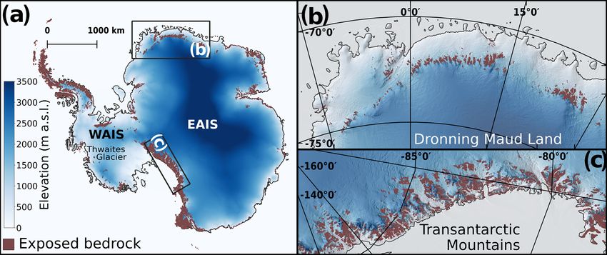
4930                                                                   M. Mas e Braga et al.: Nunataks as barriers to ice flow

2020). Near-future (2100 CE) projections of sea-level rise           ing the time of bedrock exposure allows inferring when the
point to ocean thermal expansion as the main cause (Op-              ice surface last reached the sampled elevation. In Antarctica,
penheimer et al., 2019), but over multi-centennial timescales,       most exposed bedrock is situated in regions of large topo-
the sea-level contribution from Antarctica is expected to be-        graphic relief (Fig. 1), and this is the predominant setting
come dominant (Pattyn and Morlighem, 2020). Numerical                from which rock samples are acquired (e.g. Ackert et al.,
ice sheet modelling efforts are aimed at reducing uncertainty        1999; Lilly et al., 2010; Bentley et al., 2014; Suganuma et al.,
by better understanding the processes that lead to sea-level         2014; Jones et al., 2017). Cosmogenic-nuclide exposure ages
rise, focusing on both shorter (Goelzer et al., 2020; Seroussi       are determined by the concentrations of cosmogenic nuclides
et al., 2020) and longer (Pollard and DeConto, 2009; Al-             in erratic boulders or cobbles (i.e. glacially transported clasts
brecht et al., 2020) timescales. Recent efforts include im-          of a different lithology than the underlying bedrock, de-
provements in key model components such as grounding                 posited during periods of ice cover) or bedrock surfaces. The
line dynamics (e.g. Gladstone et al., 2017; Seroussi and             concentration of a cosmogenic nuclide increases the longer a
Morlighem, 2018), coupling to solid Earth and sea-level              rock surface is exposed to cosmic rays (Gosse and Phillips,
models (e.g. Gomez et al., 2020), and improved treatment             2001). Assuming no cosmogenic nuclides have accumulated
of ice–ocean interaction processes (e.g. Reese et al., 2018;         during a previous period of exposure (i.e. an assumption of
Kreuzer et al., 2021). The importance of bedrock topography          no inheritance) and using known nuclide-specific production
(Morlighem et al., 2020) and grid resolution (Durand et al.,         rates, a measured cosmogenic-nuclide concentration can be
2011) have been acknowledged previously and studied par-             interpreted in terms of the last time the ice sheet covered that
ticularly for marginal regions of the ice sheet (e.g. Sun et al.,    specific location and consequently the ice surface elevation
2014; Robel et al., 2016; Favier et al., 2016). Spatial vari-        at the time of sample exposure or deposition. The elevation
ations in bedrock topography, as well as the resulting basal         of a sample above the present-day ice surface then enables
and lateral drag exerted at the ice–bedrock interface for dif-       determination of the magnitude of ice thinning between the
ferent spatial scales, can slow down or even stabilise ground-       time of exposure and the present. Yet, the gradient in ice sur-
ing line retreat (Jamieson et al., 2012, 2014; Åkesson et al.,       face elevation up- and downstream of a nunatak range often
2018; Jones et al., 2021; Robel et al., 2021). Regions near          does not have a clear established relationship with the re-
the ice sheet margin with large subglacial topographic re-           gional ice surface, a deficiency highlighted by Andersen et al.
lief, such as the overridden mountain ranges that fringe the         (2020). This is because (i) exposure ages provide only local
glaciated cratons of Greenland and East Antarctica (Howat            constraints regarding ice surface elevation at a particular time
et al., 2014; Burton-Johnson et al., 2016), therefore require        and (ii) considering the elevation gradient between upstream
suitable consideration when evaluating ice loss beyond this          and downstream ice surfaces, as well as an expectation that
century.                                                             these gradients will change as the ice sheet thins, it is unclear
   The accuracy of ice sheet models is limited by grid reso-         how a rock sample elevation can be consistently related to
lution (e.g. Cuzzone et al., 2019), simplifications in model         a representative regional ice surface elevation. Furthermore,
physics (Hindmarsh, 2004; Cuffey and Paterson, 2010),                when compiling cosmogenic-nuclide exposure ages sampled
and uncertainties in the climate forcing (e.g. Seguinot              around the entire Antarctic continent, it appears that there is
et al., 2014; Alder and Hostetler, 2019; Niu et al., 2019;           no systematic approach to selecting the sampling position on
Mas e Braga et al., 2021). To improve their predictive abil-         a nunatak relative to the ice flow direction around the nunatak
ity, models require validation with empirical observations.          (Fig. 2), highlighting that so far this problem has received lit-
When considering changes on multi-centennial timescales,             tle attention.
ice sheet reconstructions and ice-thinning trends in the ge-            While ice sheet models of Greenland and Antarctica have
ological past (over hundreds to thousands of years) provide          been able to broadly fit ice geometries reconstructed from
useful bounds on potential ice sheet change and important            empirical data, including the approximate rates of ice thin-
observations for constraining and testing model simulations.         ning that are recorded by cosmogenic exposure ages (e.g.
By providing empirical targets for ice sheet model simula-           Whitehouse et al., 2012; Briggs et al., 2014; Albrecht et al.,
tions, uncertain model parameters can then be fine-tuned,            2020), most models struggle to replicate the inferred tim-
and a closer match between data and models can be achieved           ing of ice thickness change (Jones et al., 2020; Stutz et al.,
(e.g. Golledge et al., 2012; Seguinot et al., 2016; Patton et al.,   2020; Johnson et al., 2021). Such data–model mismatches
2017). However, interpreting such data in terms of properly          are likely due to a combination of factors, one of which is the
providing constraints to ice sheet models, as well as using ice      spatial resolution of the models (Lowry et al., 2020; Johnson
sheet models to better interpret the data, requires a better un-     et al., 2021). When run over a glacial–interglacial cycle, ice
derstanding of the interaction between ice flow and complex          sheet models do not typically resolve the pattern of ice flow
subglacial terrain.                                                  around individual nunataks and consequently cannot resolve
   Exposed bedrock, especially where mountain summits ex-            the transient response of the ice surface at the sampled loca-
tend through the ice (i.e. nunataks), provide suitable targets       tions. We address this limitation through two tests. First, we
for cosmogenic-nuclide surface exposure dating. Determin-            test the supposition that an ice sheet up- and downstream of a

The Cryosphere, 15, 4929–4947, 2021                                                      https://doi.org/10.5194/tc-15-4929-2021

M. Mas e Braga et al.: Nunataks as barriers to ice flow                                                                               4931

Figure 1. Present-day ice surface elevation (in metres above sea level, m a.s.l.) in Antarctica (Morlighem et al., 2020). (a) The grounded
part of the Antarctic Ice Sheet, including two example settings where the East Antarctic Ice Sheet (EAIS) overrides steep subglacial terrain
of marginal mountain ranges in Dronning Maud Land and the Transantarctic Mountains (b and c, respectively), and Thwaites Glacier for
reference; (b) Dronning Maud Land, where individual nunataks and nunatak ranges tower above the ice surface; and (c) the Transantarctic
Mountains, where outlet glaciers are laterally confined by nunatak ranges. Brown areas denote exposed bedrock. Shading on panels (b) and
(c) highlights the steep surface topography.

nunatak experiences different degrees of thinning due to the            The mesh is also refined (to 500 m) in a 4 km buffer zone cen-
interaction of ice flow with an obstacle. Second, we explore            tred at the grounding line. The mean (median) element size
whether a model with horizontal grid resolutions comparable             after spin-up was 740 m (414 m).
to those currently employed by large-scale ice sheet models                In the vicinity of nunataks, where the ice is thinnest, the
(5–20 km) captures this interaction. To perform these tests,            ice flow regime has a relevant vertical component, which is
we apply a numerical ice flow model to an idealised bedrock             not captured by the SSA. A more accurate representation
topography typical of Antarctic settings.                               of the ice dynamics for such regions can be achieved with
                                                                        full-Stokes models. However, such models are currently too
                                                                        computationally demanding when adopted for long simula-
2   Data and methods                                                    tion periods and multiple experiments (e.g. Schannwell et al.,
                                                                        2020). Over the thinnest-ice areas, the horizontal scales re-
To better understand how ice flow interacts with the steep to-          solved in our model are of the order of a few hundred metres
pography of nunataks and what impact this interaction has on            (commonly noted as O(102 ) m), while the vertical scale is of
ice surface elevation patterns, we perform a suite of numeri-           the order of a few metres (O(100 ) m). This yields an aspect
cal simulations using an idealised setup. We use Úa (Gud-               ratio of O(10−2 ), which falls within the range where shal-
mundsson, 2020), an ice flow model that solves the shal-                low approximations are applicable (O(≤ 10−2 ), e.g. Fowler
low shelf, also referred to as shelfy stream approximation              and Larson, 1978). To our knowledge, no intercomparisons
(SSA or SStA) of the Stokes equations (Cuffey and Pater-                between simplified and full-Stokes models exist that focus
son, 2010), on a horizontal, finite element mesh. Úa has been           on the representation of thickness gradients. At least within
successfully applied to model the ice flow of idealised ice             the context of MISMIP+ (Cornford et al., 2020), there are
streams (e.g. Gudmundsson et al., 2012), modern ice streams             few variations between SSA (including the model used in
(e.g. Miles et al., 2021), and palaeo ice streams (e.g. Jones           our study), L1Lx, and higher-order models regarding sim-
et al., 2021). Úa solves the ice surface and momentum equa-             ulated ice retreat. Full-Stokes models that participated in
tions simultaneously, and its finite element formulation al-            the MISMIP+ experiment also agreed with the simplified-
lows for an adaptive mesh refinement in areas of particular             physics models, indicating that other models should behave
interest, such as where the ice shallows around nunataks. For           similarly. Instead, the MISMIP+ experiments highlighted the
the modelled domain (which we describe below), an unstruc-              importance of the formulation of the sliding law (i.e. Weert-
tured mesh was generated, which is refined during the sim-              man versus Coulomb-limited). The two sliding laws strongly
ulation time (including during spin-up) based on a series of            differed in their rates of grounding line retreat, but it has been
glaciological refinement criteria. Element size is refined ac-          shown that such differences decrease with increasing spatial
cording to ice thickness, from a maximum of 8 km down to                resolution (i.e. model grid/mesh refinement) at the grounding
205 m around the interface between ice and nunatak, where               line (Gladstone et al., 2017). Here, we adopt a Weertman law
ice thickness approaches the minimum (which we set as 1 m).

https://doi.org/10.5194/tc-15-4929-2021                                                        The Cryosphere, 15, 4929–4947, 2021
4932                                                                       M. Mas e Braga et al.: Nunataks as barriers to ice flow

Figure 2. (a) Polar histogram showing the location of cosmogenic 10 Be and 14 C samples from boulders in Antarctica (Heyman, 2021; Balco,
2021) with ages younger than the Last Glacial Maximum, relative to the nearest nunatak summit and its adjacent ice flow direction (n = 191;
sample duplicates were excluded). The difference in direction was computed between a sample position relative to the nunatak summit
(identified in BedMachine-Antarctica; Morlighem et al., 2020) and ice flow (Mouginot et al., 2012) near the nunatak summit. Summits were
identified through a morphological feature map (Wood, 1996, see Supplement). The area of each slice is proportional to the number of
samples within that category, and each category spans a 15◦ arc. In this figure, 0◦ (180◦ ) implies that the sample was taken downstream
(upstream), directly aligned with the ice flow direction. (b, c) kernel density function of the 10 Be (b) and 14 C ages (c) apparent exposure
ages from samples shown in panel (a). Dashed lines show the median age, and shading shows the uncertainty interval based on the median
uncertainty in their respective ages.

for basal sliding and the required refinement at the grounding           tions resolve changes in ice surface elevation across steep
line to minimise sliding-law issues.                                     ice-marginal topography under thinning scenarios and their
   At the free upper surface, the streamline upwind Petrov–              implications for simulations of past ice surface elevations.
Galerkin (SUPG) method is applied, which ensures model
stability over regions of pronounced ice surface topography              2.1   Model domain setup
(Wirbel and Jarosch, 2020). In our experiments, the ice sur-
face topography is steepest when the ice front retreats from             The model domain consists of a 300 × 200 km rectangular
the downstream end of the domain and in the vicinity of                  section of an idealised ice sheet. The domain coordinates ex-
nunataks. When ice thins below the prescribed minimum                    tend from x = −150 km to x = 150 km and y = −100 km to
(which we set to 1 m), the model uses the active-set method              y = 100 km. We create an ice cap mirrored along the x di-
(Durand et al., 2009; Gudmundsson et al., 2012). In this                 rection, i.e. where the centre of the domain (x = 0) repre-
method, violated ice thickness constraints are activated using           sents the ice divide. We apply all changes symmetrically with
the Lagrange multiplier approach (Ito and Kunisch, 2008),                respect to x but focus our analysis on the positive side of
which is applied to the momentum equation and ensures a                  the domain (i.e. x > 0; thus our effective domain is 150 km
better representation of the ice dynamics compared to sim-               long). This is done in order to ensure a natural boundary at
ply resetting the thickness to the prescribed minimum value,             the upstream side (the ice divide). The downstream side is
as is commonly used in finite element models.                            kept as an open boundary, allowing the ice front to retreat.
   The model domain (Sect. 2.1) and spin-up procedure                    On the lateral limits, a free-slip boundary condition is ap-
(Sect. 2.2) are the same for all simulations. In a first set of          plied (i.e. velocities are zero perpendicular to the boundary
simulations, we evaluate changes in ice surface elevation up-            but unconstrained parallel to it), and unless stated otherwise,
and downstream of a single nunatak under three different                 we only consider the region within 50 km of the centreline
thinning scenarios (Sect. 2.3). We then use the forcing that             (y = 0) to avoid boundary effects.
provides the highest ice-thinning rates to evaluate the im-                 We set the bed elevation at the divide (B0 ) to 750 m above
pact of multiple nunataks, as well as the width of glaciers              sea level (m a.s.l.), which we keep constant in all experi-
between them, on ice surface elevation patterns (Sect. 2.4).             ments. We prescribe a prograde sloping bed (B) with an in-
Finally, we repeat the last experiments for a series of reg-             clination β = 0.9 % (Eq. 1), which results in the bed sloping
ular meshes (without refinement) at horizontal resolutions               below sea level at x ≈ 83 km.
commonly used in ice sheet models (Sect. 2.5). This final
set of experiments assesses how well different grid resolu-
                                                                         B(x) = B0 − β · |x|                                             (1)

The Cryosphere, 15, 4929–4947, 2021                                                           https://doi.org/10.5194/tc-15-4929-2021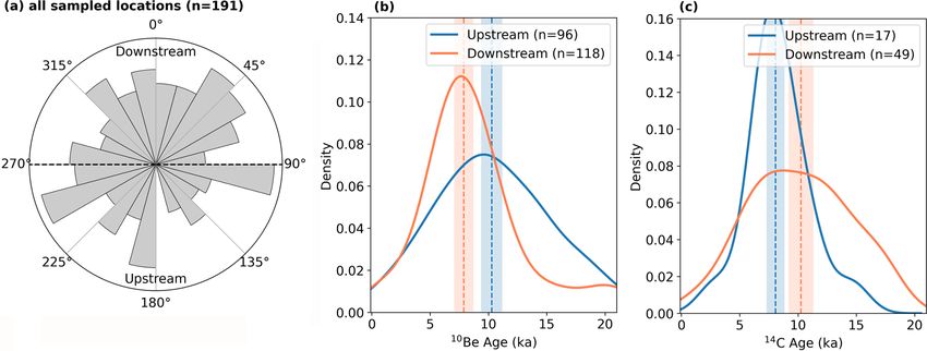
M. Mas e Braga et al.: Nunataks as barriers to ice flow                                                                              4933

   Because nunataks close to the Antarctic coast or along the       Table 1. Model parameters used in this study. Values for B0 and β
margins of palaeo ice streams are often situated in proxim-         reflect values for prograde and retrograde slopes, respectively.
ity to over-deepened troughs, which can trigger marine ice
sheet instability, a retrograde-slope case was also tested. In       Parameter                                   Value    Units
this case, we set B0 to −750 m and β to −0.1 % so that               Basal slipperiness (C)                 2.9 × 10⁻⁵    m kPa−1 a−1
the bedrock at the downstream end of the domain is at the            Weertman’s sliding law m exponent                3
                                                                     Ice temperature (for A = A(T ))               −20    ◦C
same elevation (−600 m a.s.l.) in both types of experiments,
which is representative of continental shelf depths of Antarc-       Glen’s flow law n exponent                       3
                                                                     Ice density (ρi )                              910   kg m−3
tica (Morlighem et al., 2020). The grounding line in Úa is
                                                                     Seawater density (ρw )                        1028   kg m−3
defined by the flotation condition, and although its migration       Gravity (g)                                   9.81   m s−2
is not the focus of our study, we allow it to move freely, refin-    Ice-divide SMB (a0 )                           1.3   m a−1
ing the mesh elements around the grounding line as it evolves        Domain-end SMB (ae )                          −0.3   m a−1
(as described at the end of this section).                           Ice-divide bedrock elevation (B0 )   750 and −750    m a.s.l.
   Nunataks in this domain are represented as three-                 Bedrock inclination (β)               0.9 and −0.1   %
dimensional Gaussian surfaces, which are superimposed on
B with their centre (i.e. the nunatak summit) at |x| = 50 km
and y = 0 km. All generated nunataks have an outcrop size           2.2   Model spin-up
(i.e. exposed area above the ice surface) after spin-up of ap-
proximately 12 × 5 km along their main axes. Depending on           The model spin-up starts from a 1200 m thick uniform ice
the experiment, the nunatak was elongated transversely to           distribution, to which a constant (but spatially variable) SMB
flow (i.e. along the y axis) or parallel to flow (i.e. along        is applied (i.e. b(t) = 0 m a−1 in Eq. 2) for 20 000 years
the x axis; Fig. 3). The adopted idealised nunatak dimen-           (20 kyr). This period is long enough for the system to reach
sions and the value of β are within the interval constrained        equilibrium with the SMB forcing. The average ice sur-
by 33 real nunatak topographic profiles across Antarctica           face slope between the ice divide and the grounding line
(Figs. S1–S3).                                                      (which after spin-up was located at x = 136 km; Fig. 4b)
   The effects of ice rheology (including temperature) in           is ∼ 1.3 %. This inclination is representative of measured
Úa are accounted for by the strain-rate factor A in Glen’s          profiles along nunataks for various regions of the Antarctic
flow law. To compute A, which we treat as spatially uni-            Ice Sheet (Figs. 4d, S1, S2). The resulting surface velocity
form and constant over time for the purpose of our ex-              varies from 0 m a−1 at the divide to 121 m a−1 downstream
periments, we assume an ice temperature (T ) of −20 ◦ C.            of the grounding line, with median and mean velocities of
This yields a value similar to that found for regions sur-          29 and 33 m a−1 , respectively (see Fig. S9 for a comparison
rounding nunatak escarpments in Antarctica, as obtained in          of velocity profiles along the centreline). The ice flow ve-
Gudmundsson et al. (2019) when inverting for A and basal            locity increases along the nunatak flanks, with a maximum
slipperiness (C) based on satellite-derived ice surface ve-         of ∼ 53 m a−1 , consistent with observed values in Moug-
locities. Following the same reasoning for A, we assume             inot et al. (2012). Although velocities at the floating end are
basal sliding to follow Weertman’s sliding law (Weertman,           slower than observed for ice shelves in Antarctica, they are
1957) and use a constant value for C of log10 (C) ≈ −4.5            far from our region of interest, and the setup reproduces key
(C = 2.9 × 10⁻⁵ m kPa−1 a−1 ). The main model parameters            features observed along the analysed nunatak profiles, such
are summarised in Table 1, and sensitivity analyses of values       as ice surface gradients across nunataks and ice acceleration
for A and C are presented in the Supplement (Figs. S4, S5).         upstream and downstream of the nunatak (e.g. Figs. 4, S9).
   The surface mass balance (SMB; in metres per year,               Our idealised setup focuses on capturing the key components
m a−1 ) parameterisation applied to the spin-up and subse-          mentioned above, while excluding unnecessary complex fea-
quent experiments is given by a(x, t) in Eq. (2):                   tures that could prevent identifying the ice surface response
                                                                    signal to the ice flow interaction with the obstacles.
                 a0 − ae
a(x, t) = a0 −           · |x| + b(t),                       (2)
                   Lx                                               2.3   Ice-thinning experiments
where a0 is the SMB at the ice divide (x = 0), ae is the
SMB at the edge of the domain (x = 150 km), Lx = 150 km,            In order to understand whether ice thinning occurs uniformly
and b(t) is a time-dependent SMB term through which per-            up- and downstream of a nunatak, we impose three dif-
turbations to the total SMB are applied. We prescribe a0 =          ferent degrees of ice thinning uniformly over the domain.
1.3 m a−1 , and ae = −0.3 m a−1 , which results in no ablation      The perturbations to SMB that induce ice thinning are ap-
occurring over our region of interest (black line in Fig. 4a),      plied through b(t) in Eq. (2) and only evolve in one di-
as is usual for Antarctic settings (Agosta et al., 2019).           rection over the entire domain, towards increased ablation.
                                                                    The evolution of b(t) is based on a smoothed step curve
                                                                    that applies a weight, evolving from 8 % to 100 %, mim-

https://doi.org/10.5194/tc-15-4929-2021                                                    The Cryosphere, 15, 4929–4947, 2021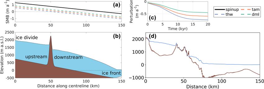
4934                                                                          M. Mas e Braga et al.: Nunataks as barriers to ice flow

Figure 3. Bedrock elevation (m a.s.l.) used in the experiments where the nunatak is placed (a) transversely and (b) parallel to ice flow. Ice
flow in this figure is from left to right. Transect lines show the position of the transects presented in Fig. 5a and b, and coloured circles show
the locations for the ice surface evolution analysis presented in Fig. 5c and d following the same colours as the lines therein.

Figure 4. Model domain setup: (a) SMB (m a−1 ) profiles for the spin-up and initial state (black) and at the end of each different ice-thinning
experiment (thw, Thwaites; tam, Transantarctic Mountains; dml, Dronning Maud Land); (b) ice surface elevation (m a.s.l.) after the 20 kyr
spin-up for the across-flow elongated nunatak; (c) applied transient perturbation (in m a−1 ) to each ice-thinning experiment during the 20 kyr
simulations subsequent to spin-up; (d) bedrock and ice sheet surface elevation profiles across an example nunatak in Antarctica (Halfway
Nunatak; 78.38◦ S, 161.1◦ E; upper Skelton Glacier, Transantarctic Mountains; see Fig. S1 for another 32 examples).

icking the deglaciation progression recorded in ocean sed-                 2.4    Three-nunatak experiments
iment and ice cores for the past 20 kyr (e.g. Lisiecki and
Raymo, 2005; Jouzel et al., 2007). This “weight curve” is                  Across much of Antarctica and Greenland, nunataks are
then multiplied by a constant chosen in order to match Last                more common in groups than in isolated cases. The aim
Glacial Maximum-to-present ice thinning at three contrast-                 of this set of experiments is therefore to test whether three
ing regions as inferred from a continent-wide transient mod-               nunataks, separated by narrow glaciers, yield ice surface el-
elling experiment (Golledge et al., 2014). These regions are               evations and gradients that differ from the control run due to
Thwaites Glacier, in West Antarctica (“thw”, −0.75 m a−1 ),                a combined effect of all the nunataks on ice flow. For this
and the Transantarctic Mountains (“tam”, −0.60 m a−1 ) and                 test, we perform sets of experiments with the same SMB
Dronning Maud Land (“dml”, −0.45 m a−1 ) in East Antarc-                   as applied in the thw experiment with one nunatak (control
tica (Fig. 4c). Using the thw scenario as an example, the                  run) but using three nunataks aligned transversely to flow at
value for b(0) is −0.75 · 0.08 m a−1 and for b(20 kyr) is                  |x| = 50 km and of the same size as in the ice-thinning exper-
−0.75 · 1.0 m a−1 . These three different thinning scenarios               iments. The spacing between nunataks differs in each exper-
were applied to nunataks that were elongated along and                     iment, resulting in glacier widths of 0 (i.e. the three nunataks
transversely to ice flow and to reference experiments with-                form a single, wider barrier), 5, 10, and 15 km. The range
out a nunatak for comparison purposes.                                     of applied widths reflects realistic values observed around
                                                                           Antarctica (Fig. S3c; Howat et al., 2019).

The Cryosphere, 15, 4929–4947, 2021                                                              https://doi.org/10.5194/tc-15-4929-2021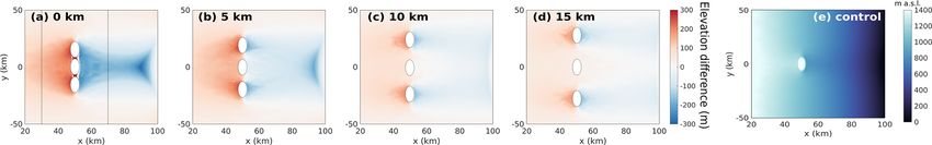
M. Mas e Braga et al.: Nunataks as barriers to ice flow                                                                       4935

2.5    Mesh-resolution experiments                                 spectively), the increase in ice surface steepening (i.e. in ele-
                                                                   vation difference) is disrupted when the downstream location
In a final series of sensitivity experiments, we assess how        becomes exposed, since its elevation no longer changes while
well regularly spaced grids of coarser resolutions typically       the equivalent point upstream is still ice covered and thin-
used in continental-scale ice sheet models (5, 10, and 20 km)      ning. This pattern of increased steepening around nunataks is
resolve the ice surface elevation pattern around nunataks          potentially important for cosmogenic-nuclide studies to con-
compared to the solution using an unstructured, locally re-        sider because from these modelling experiments, significant
fined mesh. We do so by repeating the full set of three-           differences in the time of exposure of up- and downstream
nunatak experiments and the one-nunatak thw scenario (as           faces of nunataks become apparent (Fig. 6).
control) for these regular meshes (i.e. without refinement).          To analyse the difference in timing of ice surface evolu-
   All sets of experiments, their respective surface mass bal-     tion and nunatak surface exposure up- and downstream of
ance (SMB) perturbations, and the number of nunataks in            the nunatak, we select five pairs of points equidistant from
each set are summarised in Table 2.                                the nunatak summit. They span a distance from where the
                                                                   downstream side is already exposed at the start of the exper-
                                                                   iment (1.5 km) to the closest element to the nunatak where
3     Results                                                      the ice continues to thin normally (i.e. it does not become
                                                                   exposed or stops thinning; 2.5 km) in any ice-thinning sce-
3.1    Ice-thinning experiments                                    nario. The chosen points (Fig. 6) are also separated in the
                                                                   model mesh by one element size from one another. In our
Our experiments clearly demonstrate that the presence of a         analysis, we consider that nunatak surface exposure com-
nunatak impacts ice surface elevations and that the response       mences when ice thickness falls below 10 m. A thickness
magnitude depends on its orientation relative to ice flow. The     threshold larger than the minimum thickness in the model
flow barrier created by the nunatak causes ice to accumu-          is used for a consistent identification of the timing of sur-
late upstream, depleting the downstream side of ice and caus-      face exposure between the different experiments and differ-
ing the ice surface there to lower (Fig. 5a, b). At the start of   ent points analysed, and 10 m yielded the best results among
the thinning experiments where the nunatak is placed trans-        the thresholds tested. For the purpose of cosmogenic ex-
versely to flow, the effect of the nunatak on the ice surface      posure dating, most cosmogenic-nuclide production occurs
elevation is seen up to 30 km away from its summit along           when ice is thinner than ∼ 10 m (Gosse and Phillips, 2001).
flow and 15 km perpendicularly to flow. The ice surface di-        At the upstream side, if the bedrock surface remains ice cov-
rectly upstream of the nunatak is 360 m above the general          ered according to the previous criterion, we then determine
ice sheet surface (considered to be the elevation 15 km away       when the ice surface stabilises and thus reaches its mini-
from the centreline), while downstream the lowest ice sur-         mum elevation. The implications of comparing the time of
face elevation (located 3 km downstream of the summit) is          exposure (thickness < 10 m) with time of stabilisation (thin-
100 m lower than the general ice surface elevation. Along the      ning < 5 cm/100 years) are discussed further in Sect. 4.1. For
nunatak flanks, the ice surface elevation falls about 300 m.       visualisation purposes, only the experiments with nunataks
In summary, while the general ice surface slope over the           elongated transversely to ice flow are shown in Fig. 6, but
grounded part of the domain is 1.3 %, the slope is about 2–        the patterns shown also hold true for nunataks elongated par-
3 times steeper around the nunataks. For experiments where         allel to ice flow. Because of the elongation of the nunatak,
the nunatak is elongated parallel to ice flow, the impact of       its initial area exposed along the centreline is larger, and thus
the nunatak is smaller, producing a lower ice surface eleva-       the pair of points compared for the latter are located further
tion gradient and relative elevation-change effects that can       from the nunatak summit.
be discerned 20 km up- and downstream along the centre-               The differences in the ice surface elevation between the
line and up to 5 km transversely to the centreline (Fig. 5b).      up- and downstream sides of the nunatak result in differences
In both cases, changes in ice surface elevation perpendicular      in the time of nunatak surface exposure. This occurs for all
to ice flow, caused by the nunatak presence, stand out from        scenarios but with different lags in the time of exposure de-
the general ice surface elevation for the entire extent of the     pending on the degree of thinning and distance from the sum-
subglacial nunatak obstruction (cf. Figs. 5a, b and 3a, b).        mit. For some scenarios and locations, only the downstream
   Both ice-thinning experiments detailed in Fig. 5a and b re-     side is exposed, while its upstream counterpart is still thin-
veal an overall steepening of the ice surface gradient during      ning at the end of the simulation time. Within 2 km of the
the 20 kyr thinning period (profiles from red to green). The       nunatak summit (or 6 km for the nunatak elongated parallel
evolution of this steepening is illustrated in Fig. 5c and d,      to flow) and for those scenarios where both up- and down-
where points equidistant from the nunatak summit (upstream         stream sides are exposed (or meet the stabilisation criterion),
and downstream) show ice surface elevation differences that        the upstream side lags its downstream counterpart by 2 to
increase through time. For equidistant locations closer to the     14 kyr (Fig. 6b). In a retrograde-slope setting, however, this
nunatak summit (< 2.5 and < 7.5 km for Fig. 5c and d, re-          effect is not observed. Rapid and uniform thinning happens

https://doi.org/10.5194/tc-15-4929-2021                                                  The Cryosphere, 15, 4929–4947, 2021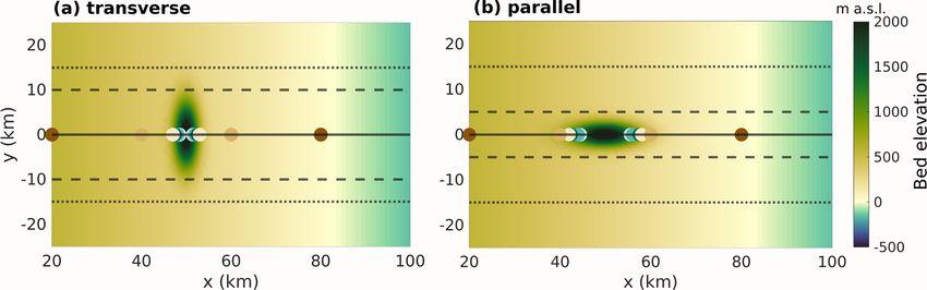
4936                                                                              M. Mas e Braga et al.: Nunataks as barriers to ice flow

Table 2. Summary of the experiments performed in this study. Adaptive mesh experiments are those that have a mesh refinement of up to
205 m around nunataks and the grounding line. Regular-mesh experiments have no refinement anywhere in the domain.

 Experiment set             No. nunataks   No. experiments                                 Nunatak aspect               b(t) at t = 20 kyr   Mesh type
                                                                                                                                  [m a−1 ]
 spinup                             0, 1   3                                               elongated across and along                 0.0    refined
                                                                                           flow and no nunatak
 thw                                0, 1   3                                               same as above                           −0.75     refined
 tam                                0, 1   3                                               same as above                           −0.60     refined
 dml                                0, 1   3                                               same as above                           −0.45     refined
 thw0y1n_mshXXkm                       1   3, with XX = [5, 10, 20] km mesh resolution     elongated across flow                   −0.75     regular XX km
 thw0y3nXXkm                           3   4, with XX = [0, 5, 10, 15] km glacier widths   same as above                           −0.75     refined
 thw0y3nXXkm_msh05km                   3   4, same as above                                same as above                           −0.75     regular 5 km
 thw0y3nXXkm_msh10km                   3   4, same as above                                same as above                           −0.75     regular 10 km
 thw0y3nXXkm_msh20km                   3   4, same as above                                same as above                           −0.75     regular 20 km

Figure 5. Surface elevations after 0, 10, and 20 kyr for the thw experiment with a nunatak elongated (a) transversely and (b) parallel to ice
flow at 0, 10, and 15 km from the centreline; dark grey lines show the respective ice surface elevation for experiments without a nunatak;
(c, d) evolution of the ice surface elevation difference between six pairs of equidistant points up- and downstream of the nunatak, along the
centreline for the experiments showcased in (a, b), respectively. In short, this figure shows to what extent a single nunatak is able to influence
ice surface elevation in space (along and perpendicularly to flow) and through time, how ice surface elevation is linked to a nunatak’s
subglacial topography, and how the ice surface elevation mismatch evolves differently depending on the distance from the nunatak.

once accelerated grounding line retreat is triggered, akin to                  merge into a single, 36 km wide nunatak; Fig. 7a) yields
marine ice sheet instability, yielding a similar adjustment up-                the highest ice retention upstream (further delaying surface
and downstream of the nunatak (Fig. S10).                                      lowering at the upstream side), with its surface up to 250 m
                                                                               higher compared to the control one-nunatak case (Fig. 7e).
3.2    Three-nunatak experiments                                               For the experiments with the smallest glacier widths (0,
                                                                               5 km; Fig. 7a, b), the constructive interference between the
The experiments with three nunataks show how differ-                           nunataks results in an ice retention that is strong enough to
ent glacier widths produce dissimilar responses of ice sur-                    instigate a strong deficit response downstream. Compared to
face elevation (Fig. 7), mimicking situations where multiple                   the control scenario, this response reaches as far as 50 km
nunataks are separated by narrow glaciers. After 20 kyr of ice                 downstream of the nunataks, also impacting the grounding
thinning, the 0 km width experiment (i.e. where the nunataks                   line position, displacing it further inland on the lee side of the

The Cryosphere, 15, 4929–4947, 2021                                                                    https://doi.org/10.5194/tc-15-4929-2021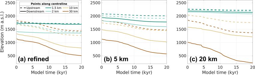
M. Mas e Braga et al.: Nunataks as barriers to ice flow                                                                           4937

                                                                        stream as the cause for the increase in relative heighten-
                                                                        ing/lowering of the ice surface.

                                                                        3.3   Mesh-resolution experiments

                                                                        The coarser regular-mesh experiments (5, 10, and 20 km
                                                                        horizontal resolution) applied to the series of three-nunatak
                                                                        configurations show important differences from the refined-
                                                                        mesh experiments (Fig. 9; cf. Fig. 7). The 5 km mesh exper-
                                                                        iments deviate the least from the refined-mesh experiments
                                                                        and capture the relationship between glacier width and the
                                                                        ice surface elevation gradient. Still, this mesh does not cap-
                                                                        ture the same magnitude of ice surface lowering downstream,
                                                                        underestimating it by as much as 80 % (100–200 m) relative
                                                                        to the refined mesh, an effect that is particularly pronounced
                                                                        close to the nunataks (cf. Figs. 9a, b and 7a, b).
                                                                           The 10 km mesh captures, to some degree, the original
                                                                        nunatak shape and consequent surface elevation increases
                                                                        upstream and decreases downstream of the nunataks (Fig. 9f–
                                                                        j). However, there are problems with both signal strength
                                                                        (under-/overestimations of at most 250 m) and location (not
                                                                        coinciding with the pattern seen in the refined-mesh experi-
                                                                        ments). In the 20 km mesh, the original nunatak shape is not
Figure 6. Relationship between distance from the nunatak summit         properly captured (Fig. 9k–o), and the large element sizes
and time of exposure (or stabilisation of the ice surface; model kyr)   cause increased heightening/lowering of ice surface elevation
for nunataks elongated transversely to ice flow under the different     to occur much farther away up- and downstream of the obsta-
thinning scenarios (see Table 2). (a) Time of exposure (in model        cles compared to their respective refined-mesh counterparts
years) for upstream (blue) and downstream (orange) points for the       (Fig. 7). Finally, the 20 km mesh yields similar results for the
different thinning experiments: thw (circles), tam (diamonds), and      0, 5, and 10 km glacier-width experiments (Fig. 9k–m) but
dml (squares). (b) As in panel (a) but showing the time difference      yields a very different response for the 15 km width experi-
between equivalent points for the cases where exposure or stabilisa-    ment (Fig. 9n), which is much more in tune with the results
tion happens for both up- and downstream points. This figure shows
                                                                        of the refined mesh. The differences between the regular-
how upstream points lag their respective downstream counterparts
(by up to 14 kyr) in all thinning scenarios.
                                                                        mesh and the refined-mesh experiments also result in differ-
                                                                        ent thinning rates between them (Fig. 10). The 20 km res-
                                                                        olution model run overestimates the rate of thinning under
                                                                        the same forcing (Fig. 10c), while the 5 km resolution model
nunatak range. For the experiments where glacier widths are             run shows values much closer to those of the refined-mesh
10 and 15 km (Fig. 7c, d), the influence of multiple nunataks           experiment, despite the underestimated thinning (Fig. 10b).
decreases but similar patterns arise, albeit with smaller dif-             The finest regular mesh tested (5 km) performs the best
ferences compared with the control experiment.                          among the regular meshes, since it partially captures the ice
   The differences in glacier width also result in different or-        flow through the widest glaciers tested (15 km wide) and best
ganisations of ice flow around the nunataks. The wider barri-           represents the effect of glacier width on ice flow constriction
ers formed by the 0 and 5 km wide glaciers yield a different            (Fig. 11). The differences between ice flow downstream and
pattern of ice flux upstream and downstream of the nunataks             upstream shown in Fig. 11 evolve similarly in the refined and
(cf. Figs. 7a, b and 8), where most of the flux is concentrated         5 km meshes but are not well represented in the 10 or 20 km
13–30 km away from the centreline. In the case of the two               meshes. The coarsest mesh (20 km) shows similar results for
experiments that have wider glaciers (10 and 15 km), ice flux           the 5 and 15 km wide glacier experiments and for the wider
also peaks further away from the centreline than in the con-            nunatak (0 km) and the 10 km wide glacier experiments. This
trol experiment but is more uniformly distributed across the            is because the coarse mesh resolution misses two nunataks
domain. Their largest flux peaks are closer to those of the             summits, which lie between two nodes. As a result, the lower
control experiment, and distinct smaller peaks occur exactly            topography that is captured by this coarse mesh becomes a
where the glaciers are located. The difference between the              subglacial continuation of the single central nunatak. This
flux downstream and upstream is inversely proportional to               also explains why the 15 km width experiment shows an ice
glacier width (i.e. the narrower the glacier, the larger the dif-       surface elevation pattern similar to that of the control run.
ference), which points to an increased retention of ice up-             Further tests indicate that the 20 km mesh only captures the

https://doi.org/10.5194/tc-15-4929-2021                                                      The Cryosphere, 15, 4929–4947, 2021
4938 M. Mas e Braga et al.: Nunataks as barriers to ice flow
Figure 7. (a–d) Difference in surface elevation (m) between each three-nunatak thw experiment of varying glacier widths (0, 5, 10, 15 km,
respectively) with respect to the one-nunatak thw control run (shown in panel e for reference), after 20 kyr of simulation. White ellipses
delineate the nunataks in each experiment, and dashed white lines in panel (a) enclose the region between them where bedrock is exposed
during this experiment. Dotted black lines in panel (a) illustrate the position of the transects shown in Fig. 8. From this figure it is clear
that a larger obstacle or a narrow glacier can increase the differential response up- and downstream of the nunataks when compared to the
single-nunatak case.
face elevation difference. Jamieson et al. (2014) showed that
much wider channels (∼ 40 km), more characteristic of ice
streams, can already provide lateral drag capable of decreas-
ing advection of ice downstream, slowing down unstable
grounding line retreat. In their fjord experiment, Frank et al.
(2021) used widths that are more similar to our narrower
glaciers (∼ 5 km) and showed that advection of ice from
wider to narrower passages, as happens in our experiments,
can be greatly slowed down by the lateral drag provided by
the nunatak flanks. The magnitude of this response in our
experiments could have been influenced by our use of uni-
form and constant ice rheology, which results in more rigid
ice in the narrow glaciers, where flow is faster (e.g. Minchew
Figure 8. Ice flux (in Gt m−1 s−1 ) across transects 20 km upstream et al., 2018). The experiments indicate that, across ice flow
(dashed lines) and 20 km downstream (solid lines) of the nunatak (i.e. along the y direction), the extent of the ice surface that
summits (x = 50 km), as illustrated in Fig. 7a. Line colours denote is impacted is more likely related to the interaction of ice
the varying widths of glaciers separating the three nunataks, while flow with the subglacial extension of the nunatak, as com-
“control” (red line) refers to the one-nunatak experiment. Note how
monly reported for different spatial and temporal scales and
the experiment where glaciers are 15 km wide yields a profile clos-
modelling setups of different complexities (e.g. Siegert et al.,
est to that of the control experiment.
2005; Durand et al., 2011; Cuzzone et al., 2019; Paxman
et al., 2020). A relative increase in the ice surface elevation
existence of three nunatak summits when they are spaced by was observed immediately downstream of the nunatak, while
glaciers that are at least 20 km wide (not shown). Still, in the lowest elevation attained was located 3 km downstream of
these tests the glaciers are not wide enough for the mesh to the nunatak summit at the start of the simulations. Although
capture their existence, and thus the results only reflect the a similar effect can be observed on the lee side of isolated
effect of a wider obstacle. nunataks in Dronning Maud Land, Mac.Robertson Land, and
the Transantarctic Mountains (Howat et al., 2019; Andersen
et al., 2020), we cannot rule out that this is a numerical ef-
4 Discussion fect, caused by artificial advection of ice downstream of the
regions where the minimum thickness constraint is violated
4.1 Ice surface response to ice flow around nunataks and thus numerically modified (e.g. Jarosch et al., 2013).
and through narrow glaciers The ice surface steepening and consequent mismatch be-
tween the up- and downstream sides of the nunatak increases
Our modelling experiments demonstrate that the magnitude as the ice thins, until the downstream side becomes exposed.
of the ice surface elevation response due to the presence of Exposure happens earlier downstream, as expected due to
nunataks is proportional to their ability to obstruct or con- lower ice surface elevation, and an equidistant point up-
strict ice flow. The nunatak orientation relative to ice flow stream becomes exposed (or has its thinning stabilised) up
or, in the experiments where three nunataks are present, the to 14 kyr later than its downstream counterpart. The rates
width of the glaciers formed between them modulates the of thinning and consequently the timing of bedrock expo-
advection of ice downstream and consequently the ice sur-
The Cryosphere, 15, 4929–4947, 2021 https://doi.org/10.5194/tc-15-4929-2021M. Mas e Braga et al.: Nunataks as barriers to ice flow 4939 Figure 9. Difference in surface elevation (m, as in Fig. 7) between each thw three-nunatak configuration (varying glacier widths) and the thw control with one nunatak (rightmost panels), for three regular-mesh resolutions of 5, 10, and 20 km. The reference experiments were also performed on a regular mesh. These panels illustrate how differential elevation changes up- and downstream of the nunataks (digitised in white based on their outcrop size, linearly interpolating the ice surface between the nodes and vertices) differ from the experiments using a refined mesh (Fig. 7) and how this mismatch decreases with increasing glacier width. Figure 10. Evolution of the ice surface at equidistant points up- and downstream of the nunatak summit along the centreline (cf. Fig. 5c, d) in control runs with one nunatak with (a) the refined mesh (first presented in Fig. 5c), (b) the 5 km regular mesh, and (c) the 20 km regular mesh. Complementing Fig. 9, this figure shows that different estimates of surface elevation in the coarser-mesh experiments also affect how elevation evolves as the ice thins and therefore the resulting thinning rates. https://doi.org/10.5194/tc-15-4929-2021 The Cryosphere, 15, 4929–4947, 2021
4940                                                                         M. Mas e Braga et al.: Nunataks as barriers to ice flow

Figure 11. Difference between ice flux (in Gt s−1 ) 20 km downstream and upstream of the nunatak summit (i.e. solid minus dashed lines in
Fig. 8) over the entire simulation time for the experiments using a refined mesh (a) and regular meshes of a 5 km (b), 10 km (c), and 20 km (d)
horizontal resolution. This figure shows how the glacier width impacts ice advection downstream of the nunataks over time for all different
model resolutions.

sure are dependent on the choice of the basal sliding coeffi-             the minimum thickness criterion, such stabilisation does not
cient. An increase of ca. 50 % in ice thinning was observed               happen because of an equilibrium of the modelled upstream
between the higher sliding and control experiments, as well               surface with the applied SMB. If the upstream surface had
as between the control and lower sliding experiments (not                 attained equilibrium, stabilisation would have happened ear-
shown). This pattern is expected given the influence of basal             lier when the imposed thinning was lower, which is the op-
sliding on the initial ice sheet geometry (Fig. S5) and high-             posite of what was observed when comparing the three thin-
lights that the exposure lags between up- and downstream                  ning scenarios. The fact that equidistant points up- and down-
sides of a nunatak observed in the real world will be site de-            stream of the nunatak are in some cases not both exposed
pendent. The choice of minimum ice thickness used in our                  also implies that important changes in ice surface elevation
model (1 m) also influences the timing of exposure at a given             might not be recorded upstream of a nunatak. The difference
point on the nunatak (Fig. S7). Although the lag times are                in time of exposure up- and downstream is also higher in the
still comparable to the range observed (2–16 and 2–14 kyr;                experiments when ice flow is further constricted by the nar-
cf. Figs. 6b and S7b), a lower minimum thickness increased                row glaciers (Fig. S11).
such lags, while a higher minimum thickness reduced them.                    Idealised experiments have the advantage that certain in-
The surroundings of nunataks are often crevassed, which re-               teractions can be easily isolated and studied, but they also
sults in a change in ice rheology. Hence, another test was car-           simplify certain phenomena that are observed in the real
ried out where the prescribed ice rheology becomes progres-               world, which could have influenced our results. For example,
sively softer towards the nunataks by a factor of 10 (Figs. S6            our setup is largely based on Antarctic settings, but the ide-
and S7). In this test, the most notable effect from the choice            alised SMB forcing deviates from what is more commonly
of ice rheology was a delay in the timing of exposure down-               observed in Antarctica in two ways. First, we prescribe ice
stream of the nunatak relative to the control case, by 0.5–               thinning through surface melting, which is more characteris-
5 kyr, but the lag times were still of the same magnitude as              tic of Greenland (e.g. Kjeldsen et al., 2015), while Antarc-
the control case (i.e. between 2 and 10 kyr). While we use                tica’s main source of mass loss is through dynamic thinning
stabilisation of thinning upstream to determine whether the               (Pritchard et al., 2009). Since mass loss only occurs down-
ice surface attained its minimum elevation before reaching                stream of the nunataks and is highest at the downstream

The Cryosphere, 15, 4929–4947, 2021                                                            https://doi.org/10.5194/tc-15-4929-2021
M. Mas e Braga et al.: Nunataks as barriers to ice flow                                                                     4941

end of the model domain, we believe that the interaction be-       tice, which allows for improved comparisons between sites,
tween ice flow and nunataks and the consequent ice surface         uses sample elevations relative to the modern ice surface ele-
elevation response were not significantly impacted by how          vation to infer past ice sheet thickness changes (e.g. Johnson
ice thinning was imposed. Second, the temporal perturba-           et al., 2008; Jones et al., 2015). A key assumption in this ap-
tions to SMB are spatially uniform, which is indeed differ-        proach is that the ice surface gradient and organisation of ice
ent from what was observed in areas of complex topography          flow around a nunatak remained the same through time. This
(e.g. Altnau et al., 2015). In regions where high mountains        assumption contradicts our modelling results, which show
act as a barrier to the advection of moisture in the atmo-         increasing ice surface gradients around nunataks during ice
sphere, total variations in SMB are significantly lower in-        sheet thinning. Our experiments further indicate that when
land of the mountain ranges compared to in coastal regions,        samples are taken upstream (downstream) of a nunatak, esti-
which means that the surface elevation gradients found here        mates of past regional ice surface elevation will be overesti-
and the lags in surface exposure/stabilisation could be higher     mated (underestimated). In directions transverse to ice flow,
in non-idealised settings. A final set of sensitivity experi-      the ice surface is typically at a lower (higher) elevation than
ments (Fig. S8) shows that the ice surface elevation differ-       directly upstream (downstream) of the nunatak summit. The
ence between locations equidistant up- and downstream of           interpretation of thickness evolution is further complicated
a nunatak is more sensitive to the spatial gradient of pre-        considering that the direction of ice flow could have changed
scribed SMB than to the absolute values of SMB. We do              as the ice thinned (e.g. Fogwill et al., 2014; Suganuma et al.,
not consider glacial isostatic adjustment (GIA) in our ex-         2014). This means that using the present-day ice surface as
periments. Bedrock topography evolves through time due to          reference elevation could lead to misleading results.
changes in ice loading, which can influence the sensitivity of        An alternative practice for inferring ice thickness changes
the ice sheet to sea-level forcing, potentially impacting the      is to determine minimum and maximum estimates. In a re-
grounding line position (Whitehouse et al., 2019), and the         cent study by Andersen et al. (2020), three estimates were
cosmogenic production rate, possibly impacting the calcu-          provided to put bounds on ice thickness changes, recognising
lated exposure ages (Jones et al., 2019). In terms of patterns     that ice covering the sampled sites could have been sourced
of exposure up- and downstream of nunataks, the influence          locally (from nearby higher terrain), regionally, or distally
of differential isostatic bedrock uplift rates on each side of     (the latter two referring to a thickening of the nearby ice
the nunatak is much smaller than the changes in ice surface        stream Jutulstraumen). For minimum estimates of required
elevation considered here, since bedrock elevation changes         thickening to reach the sampled elevation, two reference
due to GIA happen at a spatial scale larger than the ∼ 60 km       points on the present-day ice surface were determined. A “lo-
observed in our experiments (e.g. Ivins and James, 2005).          cal” reference point was defined by the lowest elevation in
Despite the simplifications mentioned above, important in-         locally sourced ice surrounding a nunatak. A “regional” ref-
sights can be drawn from our idealised experiments regard-         erence point was defined by the major “break-in-slope” (An-
ing the impact of nunataks on ice flow patterns and how the        dersen et al., 2020) between the adjacent ice stream surface
differential response between the upstream and downstream          and more stagnant ice flanking the sampled nunatak (nor-
surfaces introduces a bias into the timing of bedrock surface      mally within 1–2 km of the nunatak). For a maximum esti-
exposure around the nunatak. These effects are important for       mate of thickening, the lowest point on the ice stream served
the interpretation of cosmogenic-nuclide exposure ages and         as reference (lowest point along a 100 km profile perpendic-
for comparing such ages with results from ice sheet models         ular to ice flow in the ice stream and across the sampled
and are discussed in more detail next.                             site). We find that these estimates of minimum and maximum
                                                                   thickening are qualitatively comparable to our modelling re-
4.2   Implications for the interpretation of past ice sheet        sults. Minimum estimates are similar to the difference be-
      reconstructions                                              tween sample elevation and reference ice surface elevation
                                                                   for samples on the downstream side of nunatak summits.
The steepening of the ice surface around nunataks has impor-       Conversely, maximum estimates could yield overestimated
tant implications for the interpretation of in situ constraints    thickness changes of several hundreds of metres – in this
on past ice thickness changes from surface exposure dating.        sense it is comparable to samples from the upstream side of
A commonly adopted practice is to assume that regional ice         the nunatak summits in our experiments, when referenced to
surface elevations are directly reflected by the absolute eleva-   the lowest-elevation present-day ice surfaces, usually down-
tions of samples, but this is likely to yield inaccurate results   stream of the nunatak or along the ice stream.
for past ice sheet reconstructions. Our study demonstrates            Our modelling results can also be used to guide the col-
that this assumption would often yield an error of up to al-       lection of samples for cosmogenic dating. Typically, nunatak
most 400 m (see Fig. 5), which is of the same magnitude            flanks are likely to provide the most accurate estimates of
as many reported thickness-change estimates in regions of          regional ice sheet thickness change, as these areas are least
significant ice surface relief (e.g. Ackert et al., 2007; Sug-     impacted by differences in ice surface steepening (cf. dashed
anuma et al., 2014; Kawamata et al., 2020). A different prac-      coloured lines and dotted black line in Fig. 5a, b and

https://doi.org/10.5194/tc-15-4929-2021                                                 The Cryosphere, 15, 4929–4947, 2021
You can also read


