Motion of finite-size spheres released in a turbulent boundary layer
←
→
Page content transcription
If your browser does not render page correctly, please read the page content below
Motion of finite-size spheres released in a turbulent boundary layer
                                                                            Yi Hui Teea,∗, Diogo Barrosa,b , Ellen K. Longmirea
                                                              a
                                                                  Aerospace Engineering and Mechanics, University of Minnesota, Minneapolis, USA
                                                                            b
                                                                              Aix Marseille Université, CNRS, IUSTI, Marseille, France
arXiv:2002.00489v2 [physics.flu-dyn] 15 Sep 2020

                                                   Abstract

                                                   Individual magnetic wax spheres with specific gravities of 1.006, 1.054 and 1.152 were re-
                                                   leased from rest on a smooth wall in water at friction Reynolds numbers, Reτ = 680 and 1320
                                                   (sphere diameters d+ = 58 and 122 viscous units, respectively). Three-dimensional tracking
                                                   was conducted to understand the effects of turbulence and wall friction on sphere motions.
                                                   Spheres subjected to sufficient mean shear initially lifted off of the wall before descending
                                                   back towards it. These lifting spheres translated with the fluid above the wall, undergoing
                                                   saltation or resuspension, with minimal rotations about any axis. By contrast, spheres that
                                                   did not lift off upon release mainly slid along the wall. These denser spheres lagged the fluid
                                                   more significantly due to greater wall friction. As they slid downstream, they began to roll
                                                   forward after which small repeated lift-off events occurred. These spheres also rotated about
                                                   both the streamwise and wall-normal axes. In all cases, the sphere trajectories were limited
                                                   to the buffer and logarithmic regions, and all wall collisions were completely inelastic. In the
                                                   plane parallel to the wall, the spheres migrated in the spanwise direction about 12% of the
                                                   streamwise distance traveled suggesting that spanwise forces are important. Variations in
                                                   sphere kinematics in individual runs were likely induced by high and low momentum zones
                                                   in the boundary layer, vortex shedding in the sphere wakes, and wall friction. The repeated
                                                   lift-offs of the forward rolling denser spheres were attributed to a Magnus lift.
                                                   c 2020. This manuscript version is made available under the CC-BY-NC-ND 4.0 license;
                                                   http://creativecommons.org/licenses/by-nc-nd/4.0/.
                                                   Keywords: Particle tracking, Particle-laden flow, Turbulent boundary layer

                                                   Preprint submitted to International Journal of Multiphase Flow                       September 17, 2020
c 2020. This manuscript version is made available under the CC-BY-NC-ND 4.0 license.
http://creativecommons.org/licenses/by-nc-nd/4.0/
1. Introduction
Particle-laden turbulent flows occur in many applications ranging from industrial pro-
cesses to the environment such as the pollutant particles in atmosphere, rivers and oceans
(e.g., Olsen et al., 1982; Law and Thompson, 2014; Castañeda et al., 2014). In a wall-
bounded flow, the particle motion is complicated by interactions with both multiple scales
in the turbulent flow and the wall itself. The presence of coherent structures such as the
alternating high and low momentum regions associated with ejection and sweep events in
the near-wall regions (Wallace et al., 1972) can induce complex particle-turbulence interac-
tions. When a particle is larger than the smallest fluid eddies, it can experience variations in
shear and normal forces around its circumference. Additionally, wall friction and restitution
can affect both the translation and rotation of the particles. Depending on the surrounding
conditions, particles can either collide with or lift off from the wall or slide or roll along
it. All these effects can significantly impact particle resuspension, deposition and transport
which are all very crucial in modeling the particle response in real applications.
Various early experiments examined particle dynamics in turbulent open-channel flows.
Among others, Sutherland (1967) investigated how grains in a sediment bed were brought
into motion by the fluid. He proposed an entrainment hypothesis whereby strong turbu-
lent eddies could disrupt the viscous sublayer and lift the grain off of the bed. Francis
(1973) and Abbott and Francis (1977) observed rolling, saltation and suspension behavior
of heavy grains transported over a planar rough bed. Meanwhile, Sumer and Oğuz (1978)
and Sumer and Deigaard (1981) observed that a sand-coated wax sphere with diameter
of approximately 30 viscous units (d+ ) propagated upwards and downwards repetitively
+
throughout its trajectory in both rough and smooth beds. Hereafter, the symbol is used
to denote quantities normalized by the friction velocity (uτ ) and the kinematic viscosity (ν)
of water at 20◦ C.
To better understand particle-turbulence interactions in wall-bounded flows, direct visu-
alization techniques were incorporated in investigations by Rashidi et al. (1990), Kaftori et al.
∗
Corresponding author
Email address: teexx010@umn.edu (Yi Hui Tee)c 2020. This manuscript version is made available under the CC-BY-NC-ND 4.0 license.
http://creativecommons.org/licenses/by-nc-nd/4.0/
(1995a,b), Niño and Garcı́a (1996), van Hout (2013) and Ebrahimian et al. (2019) to name
a few. These studies concluded that particle resuspension and deposition events in the near-
wall regions were strongly influenced by coherent flow structures. Specifically, van Hout
(2013) reported that in his time-resolved particle image velocimetry (PIV) and particle
tracking velocimetry (PTV) experiments, all lift-off events of polystyrene beads (d+ = 10)
at friction Reynolds number, Reτ = 435 were due to ejection events generated by passing
vortex cores and positive shear. Once lifted beyond the viscous sublayer, the particles either
stayed suspended in the fluid or saltated along the wall depending on the type of coher-
ent structures that they encountered. Ebrahimian et al. (2019), who studied glass beads
(d+ = 6.8) in channel flow with Reτ = 410, found the strongest bead accelerations were
correlated with fluid ejections and occurred at a wall-normal location of y + = 30. Sweep
motions contributed to streamwise decelerations of beads closer to the wall (y + < 20). In
addition, Rashidi et al. (1990) and Kaftori et al. (1995a,b), who investigated spanwise mo-
tions in dilute particle suspensions in turbulent boundary layers, concluded that the small
particles tended to accumulate in the low-speed zones where ejection events were prominent.
A key factor in particle saltation and resuspension is the lift force acting on a particle.
Sphere lift can result from mean shear (Saffman, 1965), individual vortices (Auton, 1987),
or turbulence (Sutherland, 1967) in the fluid, from solid body rotation (Magnus, 1853)
or a combination of both (see reviews by Loth, 2008 and Shi and Rzehak, 2019). When
a sphere is close to a wall, the surrounding flow field is distinctly different from that in
an unbounded flow. Hall (1988) and Mollinger and Nieuwstadt (1996), who measured the
fluid-induced forces acting on a particle fixed to the wall in a turbulent boundary layer
using force transducers, reported strong positive mean force in the wall-normal direction.
Hall’s (1988) experimental data showed that, for 3.6 < d+ < 140 and particle Reynolds
number, 6.5 < Rep < 1250, the normalized mean force could be approximated by Fy+ =
(20.90 ± 1.57)(d+ /2)2.31±0.02 . On the other hand, Zeng et al.’s (2008) fully-resolved direct
numerical simulation (DNS) of the flow over a fixed sphere located a distance above the
wall showed the opposite. The mean wall-normal forces, evaluated by integrating the non-
dimensional pressure and viscous stress around the sphere surfaces, were negative for allc 2020. This manuscript version is made available under the CC-BY-NC-ND 4.0 license.
http://creativecommons.org/licenses/by-nc-nd/4.0/
spheres with 3.56 ≤ d+ ≤ 24.94 centered at a wall-normal location of y + = 17.81 at Reτ =
178.12. Tomographic PIV performed by van Hout et al. (2018) also suggested a negative
wall-normal contribution on a tethered sphere with d+ = 50 centered at y + = 43 above the
wall at Reτ = 352 due to the sphere wake tilting away from the wall. These results imply
that the net wall-normal force including the lift force can vary significantly depending on
the gap between sphere and wall.
While the presence of a wall can affect the lift force acting on a non-rotating parti-
cle considerably, it can also cause the sphere to roll due to frictional torque. In addition,
the hydrodynamic torque generated by strong velocity gradients, vorticity and turbulent
fluctuations can also cause the sphere to rotate (e.g., Saffman, 1965; Cherukat et al., 1999;
Bagchi and Balachandar, 2002; Bluemink et al., 2008). In turbulent boundary layer flows,
White and Schulz (1977) and Niño and Garcı́a (1994), among others, evaluated the signif-
icance of Magnus lift on saltating particles based on comparisons between theoretical and
experimental particle trajectories. They concluded that Magnus lift could be a non-negligible
part of the overall particle lift force. However, rotation was not quantified in either study.
In many previous numerical simulations of wall-bounded flows, particles were mod-
eled as point-masses with no volume and thus no rotation (e.g., Pedinotti et al., 1992;
Dorgan and Loth, 2004; Soldati and Marchioli, 2009). Particle-resolved simulations are rel-
atively limited due to the high computational cost and challenges in getting fine resolution
(Balachandar and Eaton, 2010). In most of the particle-laden wall-bounded flow simula-
tions, even though finite-size effects were taken into account, effects due to particle rotation
were neither considered nor discussed explicitly (e.g., Pan and Banerjee, 1997; Zeng et al.,
2008; Fornari et al., 2016). Several studies including those from Zhao and Andersson (2011),
Ardekani and Brandt (2019) and Peng et al. (2019), reported that particle rotation can in-
duce significant effects on the turbulence modulation and should not be neglected.
Several experimental techniques have been proposed to measure sphere translation and
rotation simultaneously. For example, Zimmermann et al. (2011) and Mathai et al. (2016)
extracted the sphere position and absolute orientation by comparing the sphere images
with unique patterns captured from two perpendicular cameras to a database of syntheticc 2020. This manuscript version is made available under the CC-BY-NC-ND 4.0 license.
http://creativecommons.org/licenses/by-nc-nd/4.0/
projections. Meanwhile, Klein et al. (2013) and Barros et al. (2018) tracked the markers
embedded within or painted over the surface of a sphere using multiple cameras. Then, the
angular velocity was computed based on the optimal rotation matrix that best aligned the
tracked markers (Kabsch, 1976, 1978).
As presented above, in a particle-laden wall-bounded turbulent flow, the particle-turbule-
nce and particle-wall interactions are complicated to resolve. In the context of particle
motion, most attention has been devoted to the two-dimensional translational behavior
of particles over short streamwise distances, with little attention to rotation. In order to
comprehend the particle dynamics more fully, we track individual spheres over significant
streamwise distances while resolving all components of translation and rotation. Multiple
sphere densities and flow Reynolds numbers are considered to study the effects of specific
gravity and mean shear on sphere motions. Barros et al.’s (2018) methodology is adapted to
the requirements of the current experimental setup to reconstruct both the sphere position
and orientation. The paper is organized as follows: Section 2 describes the experimental
setup, parameters, reconstruction of particle motion and uncertainty analysis; in Section 3,
we present the results on sphere translational and rotational kinematics, and discuss how
they are affected by both turbulence and the bounding surface; the concluding remarks are
summarized in Section 4.
2. Methodology
2.1. Experimental Setup
The experiments were conducted in a recirculating water channel facility at the University
of Minnesota. The channel test section, which is constructed of glass, is 8 m long and 1.12 m
wide. A 3 mm cylindrical trip-wire was located at the entrance of the test section to trigger
the development of a turbulent boundary layer along the bottom wall. Further details on the
facility can be found in Gao (2011). Hereafter x, y and z define the streamwise, wall-normal,
and spanwise directions, respectively.
To achieve a repeatable and controllable initial condition, magnetic spheres, with diame-
ter (d) of 6.35 ±0.05 mm, molded from a mixture of blue machinable wax (913.7 kg m-3 ) andc 2020. This manuscript version is made available under the CC-BY-NC-ND 4.0 license.
http://creativecommons.org/licenses/by-nc-nd/4.0/
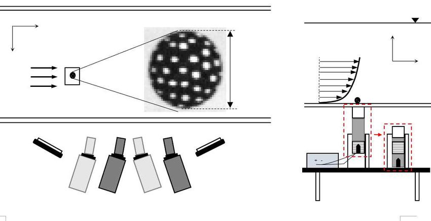
Fig. 1: Experimental setup. (a) Top view: two pairs of high-speed cameras (S1 and S2) aligned in stereoscopic
configurations for capturing the trajectory and rotation of a marked sphere over a long field of view. Inset:
example of sphere captured in grayscale with diameter, d spanning 43 pixels or 6.35 mm. (b) Side view:
sphere on smooth glass wall in a turbulent boundary layer. Red boxes illustrate the mechanism used in
holding (solenoid ON) and releasing (solenoid OFF) the sphere, respectively.
synthetic black iron oxide (5170 kg m-3 ) were used. Here, a small piece of wax was melted
inside two hemisphere molds and different amounts of iron oxide particles were added to
control the sphere density. Then, the two molds were brought together and chilled immedi-
ately to solidify the liquid wax. The resulting spheres were black and opaque. Small markers
were painted at arbitrary locations all over the sphere surface using a white oil-based pen for
good image contrast (see Fig. 1a). Both the mean inter-marker spacing and mean marker
diameter were approximately 0.6 mm.
For each run, a given sphere was held statically on the smooth glass wall in the boundary
layer by a magnet at a location 4.2 m downstream of the trip wire and 0.3 m (approximately
4 boundary layer thicknesses, δ) away from the nearest sidewall based on the sphere centroid.
This location will be considered as the origin in x and z, with the bottom wall as y = 0.
A DC 12V 2A push-pull type solenoid from Uxcell was used to hold the cubic neodymium
magnet (N40) and the sphere in position. When activated, the solenoid held the plunger suchc 2020. This manuscript version is made available under the CC-BY-NC-ND 4.0 license.
http://creativecommons.org/licenses/by-nc-nd/4.0/
that the magnet which was connected through a slider will be flush with the outer channel
wall. By switching off the power supply, both the plunger and the magnet were retracted
with the help of gravity (see Fig. 1b). As the magnet moved away from the bottom wall, the
sphere was released, allowing it to propagate with the incoming flow. A coarse screen was
located at the end of the test section to capture the sphere and prevent it from recirculating
around the channel.
Two pairs of Phantom v210 high-speed cameras from Vision Research Inc. were ar-
ranged in stereoscopic configurations to track the sphere in three-dimensional (3D) space
over a relatively long field of view. The angle between the two stereoscopic cameras was set
to approximately 30◦ for both camera pairs. The cameras were positioned with a stream-
wise overlapping distance of approximately two particle diameters in between their fields
of view. All cameras were fitted with 105 mm Nikon Micro-Nikkor lenses with aperture
f /16. Scheimpflug mounts were added to all cameras so that the images were uniformly
focused across the fields of view. Three white LED panels positioned above the cameras
illuminated the domain considered. Prior to running the experiments, the optical system
was calibrated by displacing a two-level plate (LaVision Type 22) across nine planes in the
spanwise direction for both camera pairs. A third order polynomial fit was obtained for each
plane from both cameras pairs using the calibration routine of Davis 8.4 (LaVision GmbH)
to generate the mapping function of the volumetric calibration respectively. The root mean
square (r.m.s.) error of the grid point positions was between 0.05 and 0.1 pixels indicating
an optimal fit. Image sequences were captured at a sampling frequency of 480 Hz with image
resolution of 1280 by 800 pixels, pixel depth of 12-bit, and camera pixel size of 20 µm.
2.2. Experimental Parameters
To understand the effect of turbulence, the experiments were conducted at two flow
Reynolds numbers. Here, the mean flow statistics of the unperturbed turbulent boundary
layers at the initial sphere location were determined from planar PIV measurements in
streamwise wall-normal planes. A New Wave Solo II Nd:YAG 532 nm double-pulsed laser
system with pulse energy of 30 mJ was used for illumination. The laser sheet illuminatedc 2020. This manuscript version is made available under the CC-BY-NC-ND 4.0 license.
http://creativecommons.org/licenses/by-nc-nd/4.0/
Table 1: Summary of turbulent boundary layer properties.
U∞ [m s-1 ] uτ [m s-1 ] δ [mm] Reτ Reθm
0.215 0.0092 ± 0.0001 73 ± 2 680 ± 20 1870 ± 20
0.488 0.0193 ± 0.0002 69 ± 2 1320 ± 40 3890 ± 40
through the bottom glass wall had a thickness of 1 mm. The flow was seeded with silver-
coated hollow glass spheres from Potters Industries LLC with an average diameter and
density of 13 µm and 1600 kg m-3 , respectively. At both flow Reynolds numbers, 2000
image pairs were acquired using a TSI Powerview Plus 4MP 16-bit PIV camera with camera
pixel size of 7.4 µm. The image pairs were captured at a sampling frequency of 1.81 Hz with
image resolution of 2048 by 2048 pixels.
The PIV images were processed using Davis 7.4 (LaVision GmbH) to obtain the velocity
vectors. Normalized cross-correlation (Fincham and Spedding, 1997) with an overlap of
50% over initial interrogation window sizes of 64 by 64 pixels followed by three passes of
32 by 32 pixels were employed. All vectors were post-processed with the universal outlier
detection criterion (Westerweel and Scarano, 2005) to remove spurious vectors. By applying
the Clauser chart method using log-law constant B = 5 and von Kármán constant κ = 0.41,
uτ were estimated to be 0.0092 and 0.0193 m s-1 (Clauser, 1956; Monty et al., 2009). At a
water depth of 0.394 m under both fluid conditions, the free-stream velocities (U∞ ) were
0.215 and 0.488 m s-1 , with δ of 73 and 69 mm estimated based on the mean unperturbed
streamwise fluid velocity location of U(δ) = 0.99U∞ . This corresponded to friction and
momentum thickness Reynolds numbers of Reτ = uτ δ/ν = 680 and 1320 and Reθm =
U∞ θm /ν = 1870 and 3890, respectively where θm is the momentum thickness. The spatial
resolutions of the computed velocity vectors were 14 and 29 viscous units at Reτ of 680 and
1320, equivalent to 1.51 mm. The boundary layer properties are summarized in Table 1
while the mean flow statistics are plotted in Fig. 2. The PIV streamwise velocity statistics
showed good agreement with the DNS results of Jiménez et al. (2010).c 2020. This manuscript version is made available under the CC-BY-NC-ND 4.0 license.
http://creativecommons.org/licenses/by-nc-nd/4.0/
Fig. 2: Statistics of the unperturbed turbulent boundary layers. (a) Mean streamwise fluid velocity and (b)
r.m.s. of streamwise velocity fluctuations. Lines: DNS profiles from Jiménez et al. (2010). Symbols: PIV
data. Blue: Reτ = 680; Red: Reτ = 1320. Error bars in (b) indicate the measurement uncertainties.
Spheres with d = 6.35 ± 0.05 mm and specific gravities (ρp /ρf ) of 1.006 (P1), 1.054 (P2)
and 1.152 (P3) were considered, where ρp is the sphere density and ρf is the fluid density.
This corresponds to d+ = duτ /ν of 58 and 122 viscous units, which are comparable to 26
and 46 times the Kolmogorov length scale (η) in the logarithmic region (Pope, 2000). For
each sphere, the density was determined based on the settling velocity (Vs ) measured from
high-speed imaging of the sphere falling in a quiescent fluid where ρp = 3CD ρf Vs2 /4dg + ρf .
Here, CD refers to the drag coefficient obtained from the standard drag curve (Clift et al.,
1978) while g is the gravitational acceleration. For all spheres, the uncertainty in density was
less than 1%. Meanwhile, the initial particle Reynolds numbers defined as Rep = Urel d/ν
were 760 and 1840, where Urel = 0.122 and 0.292 m s-1 are the relative velocity between
particle and mean fluid at the particle center upon release. In our cases, Stokes numbers
(Skη ), expressed as the ratio of the particle’s response time, τp = (ρf +2ρp )d2 /36νρf (Crowe,
2005) to the characteristic flow time scale based on Kolmogorov, τη (Pope, 2000), ranged
from 59 to 193. Note that although |Vs |/U∞ is relatively small for sphere P1, it is very
significant for P2 and P3. Details of the experimental parameters are summarized in Tablec 2020. This manuscript version is made available under the CC-BY-NC-ND 4.0 license.
http://creativecommons.org/licenses/by-nc-nd/4.0/
∗
Table 2: Summary of experimental parameters. Fy = (Fy − Fb )/Fb where Fy and Fb denote the mean
wall-normal fluid-induced force based on Hall’s (1988) expression and the net buoyancy force, respectively.
U (y = d2 ) ∗
Reτ Initial Rep d+ Sphere ρp /ρf Skη |Vs |/U∞ Initial Fy
[m s-1 ]
680 0.122 760 58 ± 2 P1 1.006 ± 0.003 59 0.081 12 ± 2
P2 1.054 ± 0.006 60 0.43 −0.20 ± 0.12
P3 1.152 ± 0.015 64 0.74 −0.74 ± 0.04
1320 0.292 1840 122 ± 5 P1 1.006 ± 0.003 176 0.036 72 ± 12
P2 1.054 ± 0.006 181 0.19 3.4 ± 0.7
P3 1.152 ± 0.015 193 0.33 0.45 ± 0.24
2. The particles were tracked over a streamwise distance up to x ≈ 5.5δ. For each case
considered, R = 10 trajectories were captured using the same sphere. For spheres P1 and
P3, an additional 55 and 65 runs respectively were completed at both Reτ to track the initial
sphere lift-off behavior.
2.3. Reconstruction of Particle Translation and Rotation
Before computing the particle translation and rotation, the grayscale images were first
pre-processed using Matlab to isolate the sphere from the background. A standard circular
Hough Transform routine was applied to locate the sphere. Next, the background surround-
ing the sphere was removed by setting the intensity values to 0 (black). The extracted sphere
images were then imported to Davis 8.4. Here, the images were further processed with 3 x
3 Gaussian smoothing and sharpening filters to increase the dot contrast. Pixel intensity
values that were less than those of the white dots were set to 0 to isolate the dots from the
sphere image. In all images, the minimum digital dot size was approximately 2 x 2 pixels.
Subsequently, a 3D-PTV routine based on the volumetric calibration mapping function was
implemented to reconstruct the dot coordinates from both camera pairs.
The data sets obtained from the PTV were composed of the 3D coordinates of true andc 2020. This manuscript version is made available under the CC-BY-NC-ND 4.0 license.
http://creativecommons.org/licenses/by-nc-nd/4.0/
ghost markers and their corresponding 3D velocity vectors. Hence, the filtering methodology
proposed by Barros et al. (2018) was employed to remove the ghost tracks. Once the true
markers had been determined, the sphere centroid was determined by applying the equation
of a sphere. Then, a rotation matrix that best aligned the markers of consecutive images was
obtained by applying Kabsch’s (1976) algorithm. In all runs, at least 8 markers were retained
when computing the sphere centroid locations and rotation matrix. Even though all spheres
were captured at 480 Hz, different processing frequencies were used in tracking. Depending
on the sphere translation speed, the processing frequency was optimized to ensure that
marker displacement between images was larger than the disparity uncertainty (see Section
2.4) while limiting maximum sphere streamwise displacement to less than 10 pixels to avoid
false marker pairing. More details of the reconstruction process can be found in Barros et al.
(2018).
2.4. Uncertainty Analysis
For the PIV measurements, the random errors of the mean velocity vector in both cases,
computed based on a 95% confidence interval, were less than 0.2% of the local mean velocity.
For the r.m.s. of the streamwise velocity fluctuations (urms ), the corresponding maximum
statistical uncertainty estimated based on chi-square analysis with a 95% confidence interval
was 3% (see the errorbars plotted in Fig. 2b). The accuracy of δ is limited by the PIV
vector spatial resolution and this gives an uncertainty of up to 3% from the estimated
value. Meanwhile, the uncertainty of uτ evaluated based on fitting the logarithm law of
the wall equation between y + > 30 and y/δ < 0.2 was approximately 1%. These resulted
in an uncertainty of 3% in the Reτ calculation. Next, the uncertainty of Reθm , which was
estimated based on the statistical error of the mean velocity data, was around 1%.
For the marker reconstruction, the mean disparity error, ǫ∗disp calculated by projecting
the 3D reconstructed markers back to the camera image in Davis 8.4, was approximately 0.8
px. This gives an estimate of the uncertainty in the marker locations due to reconstruction
errors (Wieneke, 2008). To reduce the noise in computing derivatives, the raw position and
orientation data were smoothed by a quintic spline (Epps et al., 2010). The mean uncertain-c 2020. This manuscript version is made available under the CC-BY-NC-ND 4.0 license.
http://creativecommons.org/licenses/by-nc-nd/4.0/
ties of the sphere position (x, y and z) as well as orientation (θx , θy and θz ) were computed
based on the r.m.s. between the raw and smoothed data (Schneiders and Sciacchitano, 2017).
For sphere position, the uncertainties were 0.51, 0.18 and 0.95 px; for orientation, the val-
ues were 1.2, 1.5 and 0.52 px, respectively. These correspond to mean translational and
angular displacement uncertainties of 0.01d and 1.5◦ . Lastly, the mean uncertainties of the
translational sphere velocities (Up , Vp and Wp ) were estimated to be 2%, 1% and 4% of the
respective U∞ .
3. Results and Discussion
3.1. Sphere Translation
3.1.1. Sphere Trajectories
Figure 3 shows the sphere wall-normal (y) trajectories plotted against their streamwise
distance traveled. In this section, for visual clarity, only results from four out of ten runs
(R = 4/10) are plotted for each case, unless otherwise specified. For results from all ten
runs, refer to Tee et al. (2019). The upward force required to lift a particle off and away
from the wall, which must derive from net pressure and viscous forces, must overcome the
constant downward buoyancy force, defined as Fb = (ρp − ρf )πd3 g/6, in all cases studied.
In a turbulent boundary layer, the upward force could derive from mean effects such as
mean shear or short-term effects related to local fluid motions. Depending on the velocity
field surrounding the sphere, wall-normal drag can be significant (see e.g. van Hout, 2013).
Also, if Rep is sufficiently large, i.e. greater than ∼ 100, vortex shedding off of the sphere
may generate intermittent wall-normal forces (see Zeng et al., 2008; van Hout et al., 2018).
Among these possibilities, we first consider the effect of mean shear on the initial sphere
wall-normal motion using Hall’s (1988) equation obtained for a fixed sphere in a turbulent
boundary layer such that Fy = Fy+ ν 2 ρf . If the mean wall-normal fluid-induced force is
∗
greater than the net buoyancy force, then Fy = (Fy − Fb )/Fb > 0, and the sphere is
expected to lift off upon release from rest on average (see Table 2). The uncertainty of this
equation was approximately ±0.15Fy for both flow Reynolds numbers investigated.c 2020. This manuscript version is made available under the CC-BY-NC-ND 4.0 license.
http://creativecommons.org/licenses/by-nc-nd/4.0/
Fig. 3: Samples of (R = 4/10 runs) sphere wall-normal trajectories at (a) Reτ = 680 and (b) Reτ =
1320 respectively plotted based on the centroid positions. Left axis: plotted in viscous units; Right axis:
normalized by the sphere diameter, d. Specific gravity: P1 = 1.006 (black), P2 = 1.054 (green) and P3 =
1.152 (purple).
∗
For the least dense sphere P1, at Reτ = 680, Fy = 12. Increasing Reτ to 1320 doubled
d+ so that the estimated mean force increased sixfold. These estimations correlated very well
with our observations for P1 (plotted as black in Fig. 3). At Reτ = 680, this sphere lifted
off immediately and within approximately 0.3δ or 3d in 65% and 18% of 75 runs observed,
respectively. In the remaining runs, it lifted off at downstream locations significantly greater
than 0.3δ. Meanwhile, at Reτ = 1320, this sphere always lifted off immediately upon release
in 75 runs observed. Owing to the stronger resultant upward force at higher Reτ , sphere
P1 initially rose to greater heights than at the lower Reτ in nine out of ten trajectories
reconstructed. Thus, the initial lift-off height correlated strongly with the local mean shear
(dU(y)/dy) which is 40% higher for the higher Reτ . In a recent fully-resolved DNS of
flow over a sphere initially resting on a porous rough bed, Yousefi et al. (2020) showed a
∗
resuspension case with Fy = 15 that lifted off initially up to y = 2.5d in one of the four
runs simulated.
∗
Although Fy = −0.2 at Reτ = 680 for sphere P2, it lifted off of the wall one out of
ten runs (plotted as green in Fig. 3a). In the remaining runs, this sphere mainly translated
along the wall once released. Meanwhile, at higher Reτ (plotted as green in Fig. 3b), thisc 2020. This manuscript version is made available under the CC-BY-NC-ND 4.0 license.
http://creativecommons.org/licenses/by-nc-nd/4.0/
sphere lifted off of the wall eight out of ten runs due to the stronger mean upward lift force
∗
(Fy = 3.4). At this Reτ , all initial lift-off heights were lower than those of P1.
For the densest sphere P3, at the lower Reτ , no initial lift-off was observed in 65 runs.
The sphere did not have sufficient upward lift to overcome the downward buoyance force
∗
(Fy = −0.74) and translated along the wall upon release. At the higher Reτ , although
∗
Fy = 0.45, sphere P3 lifted off of the wall only once in 65 runs.
In general, Hall’s (1988) equation provided a good estimate as to whether a sphere lifted
off initially. The variations in behavior observed for sphere P2 (and the one exception
observed for P3) are likely explained by instantaneous variations in streamwise velocity
approaching and surrounding them. The r.m.s. streamwise fluid velocities at the initial
sphere centroid positions at Reτ = 680 and 1320 were 20% and 15% of the unperturbed local
mean value respectively (see Fig. 2b). Thus, according to the Hall’s (1988) equation, the
instantaneous lift forces could vary up to 40% and 26% from Fy respectively. Similarly, the
instantaneous wall-normal drag force can vary depending on the local velocity fields. These
time-dependent variations in the lift and wall-normal drag forces, can also help explain the
large variations in initial lift-off heights observed for the lifting spheres released under the
same mean fluid condition. Finally, it is important to point out that Hall’s (1988) equation
was fitted based on experimental data up to Rep = 1250. Hence, our observations on sphere
P3 at Reτ = 1320 with Rep = 1840 suggest that Hall’s (1988) equation might over-predict
the mean wall-normal fluid-induced force for spheres with Rep > 1250.
Spheres that initially lifted off always descended towards the wall after reaching a lo-
cal maximum in height. While the net buoyancy force was downward in all cases, these
descents could be aided by changes in the wall-normal force after the spheres moved away
from the wall (see Zeng et al. (2008) and additional discussion in Section 3.1.3 below).
Sphere P1 at Reτ = 1320 either recontacted the wall and then lifted off (saltation) or else
reached a minimum height above the wall before reascending to a higher location (resus-
pension). In all other lifting cases, the spheres always recontacted the wall and then either
lifted off again (saltation) or else translated along the wall (sliding and/or rolling). These
propagation modes were previously observed by Francis (1973), Abbott and Francis (1977),c 2020. This manuscript version is made available under the CC-BY-NC-ND 4.0 license.
http://creativecommons.org/licenses/by-nc-nd/4.0/
Sumer and Deigaard (1981), Niño et al. (1994) and van Hout (2013) with particles propa-
gating over rough or smooth beds.
During either saltation or resuspension, sphere P1 frequently ascended to greater heights
than those attained after the initial release, with the maximum height observed of y ≈ 2.3d.
This behavior was observed in 10/10 and 7/10 runs investigated at Reτ = 680 and 1320
respectively. At Reτ = 680, this sphere collided with the wall and saltated more frequently
than at Reτ = 1320 where it mostly propagated above and further away from the wall. By
contrast, the maximum heights observed for spheres P2 and P3 were 0.3d or less throughout
their entire trajectories. Interestingly, sphere P3 exhibited a consistent lift-off pattern that
was different from the other spheres. Although this sphere did not generally lift off upon
release, after it had traveled along the wall a certain distance, repeated small lift-off events
began to take place (see figures 5(c, d) for better illustration). This behavior, which was
observed for both Reτ , typically began when x & 2δ. Even though sphere P1 lifted off to
a larger height than other spheres throughout the trajectories, its rising and falling angles
were always less than 12◦ , and typically stayed below 5◦ . For spheres P2 and P3, the rising
and falling angles were typically 2 − 3◦ .
3.1.2. Sphere Streamwise Velocity
Figures 4(a, b) represent the sphere mean streamwise velocities (Up ) obtained based on
averaging Up at each streamwise location over R = 10 curves for each case. Once released,
the spheres gained momentum from the hydrodynamic drag force and accelerated rapidly
with the flow. At a streamwise location close to 0.5δ, the acceleration magnitudes decreased
sharply and the spheres began to approach an approximate mean terminal velocity. From
there onward, the mean velocity curves stay relatively flat for all spheres except for sphere
P3 at Reτ = 680 where the sphere accelerated again near x ≈ 1.5δ to a new approximate
mean terminal velocity. Interestingly, even though the details of sphere motions between P2
and P3 were comparatively different, at both Reτ , their mean velocity curves tend towards
similar values. Note that in all cases, after achieving approximate terminal velocity (x > 2δ),
the statistical uncertainty in Up , estimated based on ± √tσR where σ is the standard deviationc 2020. This manuscript version is made available under the CC-BY-NC-ND 4.0 license.
http://creativecommons.org/licenses/by-nc-nd/4.0/
Fig. 4: (a, b) Sphere mean streamwise velocity, Up normalized by free stream velocity, U∞ at Reτ = 680
and Reτ = 1320 respectively. (c, d) Samples of (R = 4/10 runs) sphere streamwise velocity, Up normalized
by mean unperturbed streamwise fluid velocity (U (y)) at the height of the sphere centroid at Reτ = 680
and Reτ = 1320 respectively. Black: P1; Green: P2; Purple: P3.
and t = 2.262 for 95% confidence level, is always less than ±15% of the respective mean
value.
Considering spheres that propagated along the wall, the initial acceleration of sphere
P3 at Reτ = 680 was much smaller than for sphere P2 at Reτ = 680 and sphere P3 at
Reτ = 1320. These trends can be interpreted by taking into account the forward drag and
opposing wall friction forces acting on each sphere at the time of release. We estimate the
initial drag force using FD = πρf CD (Urel d)2 /8 where CD is the drag coefficient obtained
from the standard drag curve (Clift et al., 1978) and Urel is the initial relative fluid velocity
at the sphere centroid location. Then, the friction force, defined as Ff = fc N where fc is a
constant friction coefficient and N = Fb −Fy is the approximate normal force for a non-lifting
sphere, is computed for sphere P2 and P3. At Reτ = 680, as the sphere density increased
from P2 to P3, friction increased by an order of magnitude. Hence, sphere P3 experiencedc 2020. This manuscript version is made available under the CC-BY-NC-ND 4.0 license.
http://creativecommons.org/licenses/by-nc-nd/4.0/
stronger opposing wall friction and accelerated more weakly than P2 upon release. As Reτ
increased to 1320, the forward drag increased almost fourfold. Due to the smaller forward
drag force sphere P3 experienced at Reτ = 680 than at Reτ = 1320, its forward motion was
strongly retarded. Note also that for sphere P3, as Reτ increases, the friction force should
decrease due to the concomitant increase in Fy .
In a uniform, steady, unbounded flow, a sphere would accelerate until it approaches the
surrounding fluid velocity. However, in our studies, the presence of both turbulence and the
wall modify both the surrounding flow fields and the sphere kinematics. Based on figures
4(c, d), where Up is normalized by the mean unperturbed fluid velocity at the height of the
sphere centroid (U(y)) obtained from PIV, the sphere velocities mostly lagged behind the
local mean fluid velocity over the streamwise distance investigated. Sphere P1 came closer to
the mean local fluid velocity than the other particles, with mean velocity of approximately
0.9U(y) at both Reτ . For spheres P2 and P3, the curves began to level off around 0.6U(y)
and 0.7U(y) at Reτ = 680 and 1320 respectively. These differences are likely due to the fact
that P1 is typically detached from the wall while P2 and P3 are not. Moreover, on some
occasions, sphere P1 at both Reτ and sphere P2 at Reτ = 1320 traveled faster than the local
fluid mean.
In all runs, even after attaining an approximate terminal velocity, the individual sphere
velocity curves still fluctuate substantially. To better understand the fluctuations in the
velocity curves, sample wall-normal trajectories for sphere P1 (black) and P3 (purple) and
their corresponding streamwise velocities (blue) at both Reτ are plotted in Fig. 5. For sphere
P1, the local y-position correlates positively with the respective value of Up in all four runs
shown and in the additional runs corresponding to these cases. As sphere P1 ascended, it
gained more momentum from the faster moving fluid away from the wall and accelerated; as
it descended, it lost momentum due to the slower moving fluid near the wall and thus began
to decelerate. When we estimated the oscillating frequencies (f ) of the streamwise velocity
curves at both Reτ , in portions of runs where Rep > 100, the resulting Strouhal number,
St = f d/Urel corresponded very well with the range of 0.1 to 0.2 associated with vortex
shedding (Zeng et al., 2008; van Hout et al., 2018). This behavior was observed frequentlyc 2020. This manuscript version is made available under the CC-BY-NC-ND 4.0 license.
http://creativecommons.org/licenses/by-nc-nd/4.0/
Fig. 5: Sphere wall-normal trajectories, y + (left axis) and streamwise velocities, Up /U∞ (right axis; blue).
(a, c) Reτ = 680; (b, d) Reτ = 1320. Black: P1; Purple: P3. Solid and dashed lines in (a, b) represent two
individual runs.
for both Reτ , and in almost every run at Reτ = 680 where, downstream of x = 0.5δ, Rep
remained larger on average.
Sphere P3 always stayed close to the wall, and where the height varied during very small
lift-off events (x > 2δ), it occurs at a much shorter wavelength than the corresponding
streamwise velocity fluctuations in the same region (see figures 5(c, d)). Therefore, these
variations appear decoupled. When x < 2δ, the velocity curve for Reτ = 680 varied strongly
at St ∽ 0.2 also suggesting vortex shedding. This behavior, which was common across
all runs for this case, manifests as short wavelengths in Fig. 5c due to the relatively small
propagation speed and large relative velocity in that region. After the sphere accelerated
again at x ∼ 2δ, the vortex shedding effect was still present. At Reτ = 1320, the streamwise
velocity curves also fluctuated at the vortex shedding frequency.c 2020. This manuscript version is made available under the CC-BY-NC-ND 4.0 license.
http://creativecommons.org/licenses/by-nc-nd/4.0/
While the effect of vortex shedding on sphere streamwise velocity is important in most
of the cases studied, the simulations by Zeng et al. (2008) on a fixed sphere located above
the wall showed that the oncoming wall turbulence was also an important contributor to
fluctuations in the streamwise force on the sphere. Similarly, in some instances, the timewise
variations in velocity magnitude observed herein are likely driven by local high and low
momentum regions that surround and move past the sphere. Our preliminary findings on
planar fluid velocity fields surrounding a moving sphere at y = 0.75d have shown that
a sphere enveloped by a long streamwise region of relatively slow moving fluid traveled
significantly slower than the same sphere enveloped by relatively fast moving fluid. Thus,
the local fluid velocity variations can explain the strong variations in sphere velocity at a
given streamwise location across different runs as well as some occasions where Up /U(y) > 1.
3.1.3. Sphere Wall-normal Velocity
The wall-normal sphere velocities (Vp ) at Reτ = 1320 are plotted in Fig. 6a. Two sample
Vp curves are also plotted in blue on the right axis in Fig. 6b along with their respective
wall-normal trajectories in black on the left axis. The results show that upon release, sphere
P1 propagated with the highest Vp , up to 0.1U∞ , and hence lifted off to a greater height
than other spheres. At the same time, the oscillating frequencies of the wall-normal velocity
for P1 in Fig. 6b, as well as in the other runs where Rep were also > 100, matched very
well with the Strouhal number associated with vortex shedding. As sphere P2 has greater
density than P1, it lifted off with smaller wall-normal velocity. Although the initial Vp of
P3 was zero, after x ≈ 2δ, the curves began to fluctuate at frequencies corresponding with
St ∼ O(1) or larger, with ascending velocity of approximately 0.05U∞ . The higher values
of St imply that the small repeated lift-off events, which corresponded to the fluctuations
in wall-normal velocity, were not prompted by vortex shedding. Surprisingly, even though
sphere P3 was the heaviest sphere and lifted off less than 0.25d from the wall, it generally
reached Vp magnitudes larger than those of P2 and comparable to those of P1. Similar
wall-normal velocity trends were observed at the lower Reτ for all spheres (not shown here
for brevity).c 2020. This manuscript version is made available under the CC-BY-NC-ND 4.0 license.
http://creativecommons.org/licenses/by-nc-nd/4.0/
Fig. 6: (a) Samples of (R = 4/10 runs) sphere wall-normal velocity at Reτ = 1320, Vp normalized by free
stream velocity, U∞ . Black: P1; Green: P2; Purple: P3. (b, c) Sphere P1 at Reτ = 1320; Left axis:
wall-normal trajectories, y + (black); Right axis: sphere wall-normal velocity, Vp /U∞ and acceleration, ay,p
respectively (blue). Solid and dashed lines represent two individual runs plotted. Red line in (c) represents
ay,p = 0.
On the other hand, during descents, as shown in Fig. 6a, P1 moved towards the wall
with minimum values close to Vp ≈ −0.06U∞ , almost double its settling velocity. In most
runs, P1 descended with negative Vp value larger than or comparable to those observed
for both the denser spheres. A similar finding was observed in the numerical simulation of
Yousefi et al. (2020), where their resuspending sphere also descended with magnitude larger
than Vs value at multiple instances along its trajectory.
When the sphere was held at rest in the flow, Rep was 760 and 1840 for Reτ = 680 and
1320, respectively. After strong initial accelerations, these values decreased significantly in
all cases. Beyond x = 3δ, the average Rep values were larger for P2 and P3 (O(300) and
O(400) at Reτ = 680 and 1320 respectively) than for P1 (O(200) at both Reτ ). While
the initial lift-off events were governed mainly by the mean shear lift (as in Hall, 1988;c 2020. This manuscript version is made available under the CC-BY-NC-ND 4.0 license.
http://creativecommons.org/licenses/by-nc-nd/4.0/
Yousefi et al., 2020), the reduction in related upward force associated with the decrease
in Rep should weaken the subsequent lift-off activity. However, the resulting wall-normal
trajectories and velocities of the spheres demonstrated that the sphere lift-off heights could
be larger downstream than those upstream. This signifies the presence of a strong upward
impulse of a similar or larger value than that related to the initial mean shear lift. Similarly,
for instances where the sphere descended faster than its settling velocity, the presence of a
downward fluid impulse can be as significant as that due to the negative buoyancy force.
In this context, Zeng et al. (2008) inferred that the strong instantaneous positive and
negative wall-normal forces observed on a fixed sphere were closely associated with ejection
and sweep events. Studies by Sutherland (1967) and van Hout (2013) on moving particles, for
example, have shown that ejection events are responsible for particle lift-offs. These findings
suggest that the subsequent lift-off events of larger magnitudes observed in the current study
are likely triggered and aided by coherent fluid motions. While ejection events could provide
the sphere with upward momentum, negative wall-normal fluid motions such as sweeps could
provide the sphere with sufficient downward momentum to descend faster than its settling
velocity. Depending on the type and strength of coherent structures encountered by a
sphere, its wall-normal motion can vary significantly (as shown in Fig. 3) with the change
in instantaneous lift and wall-normal drag forces. As a reference, the r.m.s. wall normal
fluctuating velocity (vrms ) for 29 < y + < 300 could vary between 3 and 5% of U∞ at both
Reτ .
It is notable that, over the streamwise distances investigated, all sphere trajectories
were limited approximately to the buffer and logarithmic regions where turbulent activity
is strongest. Thus, although a sphere could be lifted to significant heights above the wall,
the wall-normal impulses were not sufficient to drive it to even greater heights. Considering
the nature of the impulse, it can derive from a large upward force exerted over a short time
or a smaller force exerted over a longer time. For all three spheres examined, the upward
impulse must counteract a downward one due to gravity. The wall-normal acceleration
for sphere P1 plotted in Fig. 6c revealed multiple behaviors. In one run (solid curves),
the sphere acceleration, and net impulse, was initially positive until it reached y + = 150.c 2020. This manuscript version is made available under the CC-BY-NC-ND 4.0 license.
http://creativecommons.org/licenses/by-nc-nd/4.0/
Further downstream, beginning at x = 1.3δ, the sphere again experienced a sustained upward
acceleration over the range 175 < y + < 220. By contrast, in the other run (dashed curves),
the initial upward acceleration lasted only for a short distance until the sphere rose to
y + = 80. Further downstream, however, starting at x = 1.8δ, the same sphere experienced
another upward acceleration as it rose from the wall up to y + = 140. The fact that the
turbulent activity, and the probability of sustained upward fluid motions, dies off beyond
the logarithmic region, helps explain the observed result that the spheres examined never
rose above a limit of y + = 282 (y/δ = 0.21) within the field of view investigated.
The wall-normal trajectories plotted in Fig. 3 showed that in most runs, spheres that
initially lifted off descended and collided with the wall before lifting off again. Thus, to
better understand the effect of collision on sphere lift-off events, the coefficient of restitution
(e), which is the ratio of wall-normal velocity after impact (Vf ) to wall-normal velocity before
impact (Vi ), was computed. Among all collision incidents, e was always zero. After colliding
with the wall, the spheres slid for a distance of at least 0.1d (> 3 frames) before lifting off
again. When the impact Stokes numbers, defined as Sk = ρp Vi d/18νρf , are calculated, in
all trajectories, Sk < 10. Therefore, the e = 0 result for Sk < 10 is consistent with previous
experiments on particles moving through quiescent fluid and impacting on solid surfaces
(Joseph et al., 2001; Gondret et al., 2002).
3.1.4. Sphere Spanwise Motion and Velocity
Sphere trajectories in the streamwise-spanwise plane are plotted in Fig. 7. Once released,
instead of propagating along z = 0, the spheres typically moved sideways, occasionally
reversing direction, with some crossings over z = 0. For P3 at Reτ = 680 and x < 2δ, the
spanwise trajectories exhibited shorter wavelength fluctuations than the other cases. In all
cases, the maximum spanwise distance traveled from z = 0 was approximately 12% of the
corresponding streamwise distance traveled. This magnitude is similar to that reported by
Yousefi et al. (2020) for their resuspension case where the sphere traveled mostly away from
the bed. Considering all cases, including the lifting sphere P1 at Reτ = 1320, in most runs,
the absolute spanwise migration magnitudes were comparable to or larger than the lift-offc 2020. This manuscript version is made available under the CC-BY-NC-ND 4.0 license.
http://creativecommons.org/licenses/by-nc-nd/4.0/
Fig. 7: Samples of (R = 4/10 runs) sphere spanwise trajectories, z at (a) Reτ = 680 and (b) Reτ = 1320
respectively.
Fig. 8: (a) Samples of (R = 4/10 runs) sphere absolute spanwise velocities, |Wp | normalized by free stream
velocity. Black: P1; Green: P2; Purple: P3. (b) Sphere P1 at Reτ = 1320. Left axis: spanwise trajectories,
z + (black); Right axis: spanwise velocities, Wp (blue). Solid and dashed lines correspond to the two
individual runs plotted in Fig. 6b.
magnitudes (see figures 6b and 8b).
The absolute spanwise velocities (|Wp |) for spheres at Reτ = 1320 are illustrated in Fig.
8a. Overall, |Wp | varied over larger magnitudes than |Vp |. By comparing Wp with Vp for
sphere P1 at Reτ = 1320 (see sample runs in figures 6b and 8b), including during the lift-off
events, the magnitude of Wp typically exceeded that of Vp . At the same time, the fluctuations
in Wp in both runs shown corresponded directly with those appearing in Vp at the vortex
shedding frequency. This correspondence was apparent as well in portion of other runs where
Rep > 100 as highlighted in Section 3.1.2. Despite the distinct differences in Vp curves for
spheres of different specific gravities, P2 and P3 attained values of Wp comparable to those ofc 2020. This manuscript version is made available under the CC-BY-NC-ND 4.0 license.
http://creativecommons.org/licenses/by-nc-nd/4.0/
P1 throughout their trajectories. Even though the wall-normal and spanwise velocity curves
appeared uncorrelated for both P2 and P3, the spanwise velocity curves also fluctuated at
St ∼ 0.1-0.2 suggesting vortex shedding in those cases as well. Similar spanwise velocity
trends were observed at the lower Reτ for all spheres (not shown here for brevity). For
comparison, at Reτ = 1320 and 29 < y + < 300, the fluid spanwise r.m.s. exceeds the wall-
normal r.m.s. value, e.g., at y + = 60, wrms /U∞ = 0.06 and vrms /U∞ = 0.04 (Jiménez et al.,
2010). Therefore, within the buffer and logarithmic regions, spanwise forces exerted by the
fluid can be larger than the comparable wall-normal forces (see also Zeng et al., 2008). Our
preliminary results including fluid velocity fields reveal that the sphere spanwise motion is
significantly affected by spanwise fluid drag. For example, we observed that sphere enveloped
by the low momentum region tended to travel in the spanwise direction together with the
surrounding fluid. More quantitative findings on the correlation between sphere and fluid
spanwise velocities are under investigation.
3.2. Sphere Rotation
Figure 9 depicts sphere orientation components for R = 4/10 runs of all six cases in-
vestigated. The orientations were calculated by integrating the respective angular velocities
obtained from the rotation matrix. Depending on the mode of translation, two distinct
trends were observed. Spheres that mostly traveled above the wall, namely sphere P1 at
both Reτ and sphere P2 at Reτ = 1320, rotated less than half a revolution about all axes
throughout the range examined. These weak rotations occurred mostly during the acceler-
ation stage when x < 0.5δ. Notably, even in the presence of strong initial mean shear, the
spheres did not develop any significant forward rolling motion (rotation about the negative
z-axis). Also, no significant correlations were found between rotation about the streamwise
axis (θx ) and spanwise migration. Without wall friction, these small rotations were most
likely induced by the flow structures such as individual vortices or shearing regions.
By contrast, spheres that mostly traveled along the wall, namely sphere P2 at Reτ = 680
and sphere P3 at both Reτ , developed significant rotations starting from x & 1.5δ. Upon
release, these spheres mainly slid along the wall and barely rolled. For x . 1.5δ, theirc 2020. This manuscript version is made available under the CC-BY-NC-ND 4.0 license.
http://creativecommons.org/licenses/by-nc-nd/4.0/
Fig. 9: Samples of (R = 4/10 runs) sphere orientation tracks (θx , θy and θz ) at Reτ = 1320 (a-c) and
Reτ = 680 (d-f ) , respectively.
θz magnitudes were smaller than either θx or θy , and of similar magnitude to those of the
lifting spheres. Further downstream, however, these spheres began to roll forward. This is
clearly indicated by the sharp and steady decrease of θz values in the plots. While rolling
forward, these spheres also rotated about the y-axis significantly, exhibiting coupled rotation
behavior. This wall-normal rotation could possibly be triggered by adjacent fast and slow
moving zones in the boundary layer which would generate a hydrodynamic torque about the
y-axis.
Within the field of view investigated, for the wall-interacting spheres, θx magnitudes
were the smallest when compared to θy and θz . For spheres P2 and P3 at Reτ = 680, the
fluctuations in θx curves correlated very well with the spanwise trajectories in most runs.
In figures 10 (a, d), two examples of spanwise trajectories for sphere P3 at Reτ = 680 are
plotted as purple on the left axis, while their orientations about the streamwise axis are
plotted as blue on the right axis. In both examples, when z is positive, θx is positive and
when z is negative, θx is negative. Moreover, the spanwise displacements calculated basedc 2020. This manuscript version is made available under the CC-BY-NC-ND 4.0 license.
http://creativecommons.org/licenses/by-nc-nd/4.0/
Fig. 10: Sphere P3 at Reτ = 680. Solid and dashed lines represent two individual runs. (a, d) Left axis:
sphere spanwise trajectories, z/δ (purple) and angular displacement, sz (red); Right axis: sphere rotational
angle about streamwise axis, θx (blue). (b, e) Left axis: sphere wall-normal trajectories, y + (purple); Right
axis: sphere rotational angle about wall-normal axis, θy (blue). (c, f ) Left axis: y + (purple); Right axis:
sphere rotational angle about spanwise axis, θz (blue).
on sz = θx d/2 for a pure rolling motion (plotted as red relative to the left axis) matched
very well with the z-trajectories as shown in figures 10 (a, d). This implies that the spanwise
sphere motions were induced by the streamwise rotations, and while propagating sideways,
these spheres were mostly rolling about the x-axis instead of sliding. These rotations could
possibly be initiated by quasi-streamwise vortices or spanwise motions in the fluid.
To quantify the relative importance of sliding and forward rolling, we define a dimen-
sionless rotation rate, αz = |Ωz |d/2Up , which relates the sphere rotational velocity about
the spanwise axis, Ωz to its streamwise translational velocity. If αz is 0, the sphere is under-
going pure translation or sliding in the streamwise direction; if αz is 1 and the sphere is in
contact with the wall, the sphere is undergoing pure forward rolling without slipping. The
dimensionless rotation rates were calculated based on the slope of the mean x-trajectory
and θz curves for the wall-interacting spheres. For the densest sphere P3, when x > 3δ, the
mean αz values at Reτ = 680 and 1320 were approximately 0.6 and 0.4 respectively. ThisYou can also read