Online No-regret Model-Based Meta RL for Personalized Navigation
←
→
Page content transcription
If your browser does not render page correctly, please read the page content below

Proceedings of Machine Learning Research vol 168:1–23, 2022   4th Annual Conference on Learning for Dynamics and Control

                                            Online No-regret Model-Based Meta RL for Personalized Navigation

                                        Yuda Song 1                                                                          YUDAS @ ANDREW. CMU . EDU
                                        Ye Yuan 1                                                                                  YYUAN 2@ CS . CMU . EDU
                                        Wen Sun 2                                                                                  WS 455@ CORNELL . EDU
                                        Kris Kitani 1                                                                              KKITANI @ CS . CMU . EDU
                                        1
                                            Carnegie Mellon University, 2 Cornell University
arXiv:2204.01925v1 [cs.LG] 5 Apr 2022

                                        Editors: R. Firoozi, N. Mehr, E. Yel, R. Antonova, J. Bohg, M. Schwager, M. Kochenderfer

                                                                                                Abstract
                                               The interaction between a vehicle navigation system and the driver of the vehicle can be formulated
                                               as a model-based reinforcement learning problem, where the navigation systems (agent) must
                                               quickly adapt to the characteristics of the driver (environmental dynamics) to provide the best
                                               sequence of turn-by-turn driving instructions. Most modern day navigation systems (e.g, Google
                                               maps, Waze, Garmin) are not designed to personalize their low-level interactions for individual
                                               users across a wide range of driving styles (e.g., vehicle type, reaction time, level of expertise).
                                               Towards the development of personalized navigation systems that adapt to a variety of driving
                                               styles, we propose an online no-regret model-based RL method that quickly conforms to the
                                               dynamics of the current user. As the user interacts with it, the navigation system quickly builds
                                               a user-specific model, from which navigation commands are optimized using model predictive
                                               control. By personalizing the policy in this way, our method is able to give well-timed driving
                                               instructions that match the user’s dynamics. Our theoretical analysis shows that our method is a
                                               no-regret algorithm and we provide the convergence rate in the agnostic setting. Our empirical
                                               analysis with 60+ hours of real-world user data using a driving simulator shows that our method
                                               can reduce the number of collisions by more than 60%.
                                               Keywords: Model-based RL, Online Learning, System Identification, Personalization

                                        1. Introduction
                                        Reinforcement Learning (RL) and Markov Decision Processes (MDP) Sutton and Barto (2018)
                                        provide a natural paradigm for training an agent to build a navigation system. That is, by treating
                                        the navigation system that delivers instructions as the agent and combining the vehicle and the user
                                        as the environment, we can design RL algorithms to train a navigation agent that provides proper
                                        instructions by maximizing a reward of interest. For example, we could reward the agent when it
                                        delivers accurate and timely instructions. There has been a rich line of research on applying RL in
                                        various navigation tasks, including robot navigation Surmann et al. (2020); Liu et al. (2020), indoor
                                        navigation Chen et al. (2020a, 2021a), navigation for blind people OhnBar et al. (2018), etc. In this
                                        work, we put our focus on vehicle navigation, a task also explored by the previous literature Kiran
                                        et al. (2021); Stafylopatis and Blekas (1998); Deshpande and Spalanzani (2019).
                                            However, most of the previous works only consider a static scenario, where the user (robot,
                                        vehicle or human) that receives the instructions does not change its dynamics during the deployment
                                        phases. This is not practical in the real world - in practice, the navigation system is faced with
                                        different users with changing or unseen dynamics during deployment (in our case, we could face

                                        © 2022 Y. Song, Y. Yuan, W. Sun & K. Kitani.
O NLINE N O - REGRET M ODEL -BASED M ETA RL FOR P ERSONALIZED NAVIGATION

                                                           Figure 2: Examples of dynamics changes:
                                                           left: using different vehicles (cybertruck) and
Figure 1: Different participants using different driving   different visual situations (mimicking foggy
kits in our navigation system built on Carla. Each         situations). Right: using a first-person view
participant at least interacts with the system for three   instead of a third-person view, while the latter is
hours.                                                     easier to control.

different drivers, vehicles and weather conditions everyday), which requires fast personalization of
the navigation system. However, there is little hope learning a monotonic policy that fits all (and
unseen) users. In fact, even well-established navigation systems such as Google Maps are only
designed for the average user. Thus, personalization needs to be achieved through adaptation, and
we need a policy that can quickly adapt to the incoming user. Recently, meta learning Finn et al.
(2017a); Duan et al. (2016); Finn et al. (2017b) presents a way to train policies that adapt to new
tasks by few-shot adaptation. Similarly, in our online setting, we need to focus on sample efficiency
in order to have performance guarantee, i.e., we want to adapt with as few samples as possible -
otherwise, a policy is sub-optimal as long as the adaptation is unfinished. Towards this direction,
model-based RL methods have shown promising sample complexity/efficiency results (compared
to model-free algorithms) in both theoretical analysis Sun et al. (2019); Tu and Recht (2019) and
empirical applications Chua et al. (2018); Wang et al. (2019).
    Drawing the above intuitions from meta RL and MBRL, in this work we propose an online
model-based meta RL algorithm for building a personalized vehicle navigation system. Our algorithm
trains a meta dynamics model that can quickly adapt to the ground truth dynamics of each incoming
user, and a policy can easily be induced by planning with the adapted model. Theoretically, we
show that our algorithm is no-regret. Empirically, we develop a navigation system inside the Carla
simulator Dosovitskiy et al. (2017) to evaluate our algorithm. The state space of the navigation
system is the specification of the vehicle (e.g., location, velocity) and the action space is a set of
audio instructions. A policy will be trained and tested inside the system with a variety of scenarios
(driver, vehicle type, visual condition, level of skills). Ideally, a personalized policy should deliver
timely audio instructions to each different user. We conduct extensive experiments (60+ hours) on
real human participants with diverse driving experiences as shown in Fig. 1, which is significantly
more challenging than most previous works that only perform experiments with simulated agents
instead of real humans Koh et al. (2020); Nagabandi et al. (2018b). The user study shows that our
algorithm outperforms the baselines in following optimal routes and it is better at enforcing safety
where the collision rate is significantly reduced by more than 60%. We further highlight that the
proposed algorithm is able to generate new actions to facilitate the navigation process.
    Our contributions are as follows: 1) we propose an algorithm that guarantees an adaptive policy
that achieves near-optimal performance in a stream of changing dynamics and environments. 2)
Theoretically, we prove our algorithm is no-regret. 3) We build a vehicle navigation system inside
the state-of-the-art driving simulator that could also facilitate future research in this direction. 4) We

                                                       2
O NLINE N O - REGRET M ODEL -BASED M ETA RL FOR P ERSONALIZED NAVIGATION

perform extensive real-human experiments which demonstrate our method’s strong ability to adapt
to user dynamics and improve safety.

2. Related Works
2.1. RL for Navigation System
The reinforcement learning paradigm fits naturally into the navigation tasks and has encouraged
a wide range of practical studies. In this work we focus on vehicle navigation Koh et al. (2020);
Kiran et al. (2021); Stafylopatis and Blekas (1998); Deshpande and Spalanzani (2019). Previous
work can be separated into two major categories: navigation with human interaction Thomaz
et al. (2006); Wang et al. (2003); Hemminahaus and Kopp (2017) and navigation without human
interaction Kahn et al. (2018); Ross et al. (2008). The first category includes tasks such as indoor
navigation and blind person navigation. Such tasks require considering personalization issues when
facing different users, who potentially bring drastically different dynamics to the system. Previously,
vehicle navigation is categorized into the second field since there is no human interaction. However,
in our work, we provide a novel perspective and introduce new challenges by incorporating human
drivers into the system. Thus in order for an algorithm to solve this new task, it should consider
personalization, accuracy and safety at the same time. In this work, we theoretically and empirically
show that our proposed solution could address the three key components simultaneously.

2.2. Model-based RL and Meta RL
Model-based RL and meta RL are designed to achieve efficient adaptation. MBRL aims to model
the dynamics of the environments and plan in the learned dynamics models. Prior works Sun et al.
(2019); Tu and Recht (2019); Chua et al. (2018); Song and Sun (2021) have shown superior sample
efficiency of model-based approaches than their model-free counterparts, both in theory and in
practice. For navigation with human interaction, prior works have shown promising results by
modeling human dynamics Torrey et al. (2013); Iqbal et al. (2016); Daniele et al. (2017). However,
these works do not provide any personalized navigation.
     Towards the adaptability side, meta RL approaches Finn et al. (2017a,b); Duan et al. (2016) have
demonstrated the ability to adapt to a new task during test time by few-shot adaptation. Previously,
there are also works that propose meta-learning algorithms for model-based RL Nagabandi et al.
(2018b,a); Lin et al. (2020); Clavera et al. (2018); Belkhale et al. (2021); Sæmundsson et al. (2018).
However, these methods do not have any theoretical guarantee. Additionally, it is unclear if these
works can adapt in real-world scenarios since their evaluation is based only on simulation or non-
human experiments. In contrast, the proposed method is evaluated with extensive user study (60+
hours) with real-human participants which demonstrates the method’s ability to deliver personalized
driving instructions that quickly adapts to the ever-changing dynamics of the user.

3. Preliminaries
A finite horizon (undiscounted) Markov Decision Processes (MDP) is defined by M = {S, A, P, H,
C, µ}, where S is the state space, A is the action space, P : S × A → ∆(S) is the transitional
dynamics kernel, C : S × A → R is the cost function, H is the horizon and µ ∈ ∆(S) is the initial
state distribution. In this work, we consider an online learning setup where we encounter a stream

                                                  3
O NLINE N O - REGRET M ODEL -BASED M ETA RL FOR P ERSONALIZED NAVIGATION

of MDPs {M(t) }Tt=1 . Each M(t) is defined by {S, A, P (t) , H, C, µ}, i.e., the transitional dynamics
kernels are different across the MDPs. The goal is to learn a stochastic  policy π : S → ∆(A) that
                                          π
minimizes the total sum of costs. Denote dh,µ,P (t) (s, a) = Es∼µ P(sh = s, ah = a|s0 = x, π, P (t) )


to be the probability of visiting (s, a) under policy π, initial distribution µ and transition P (t) .
     π          1 PH−1 π
Let dµ,P (t) = H h=0 dµ,h,P (t) be the average state-action distribution. Since in the online
                                                                             (t) T , the value at round
                     hP incurs a sequence of (adapted)ipolicies π = {π }t=1
setting, if the algorithm
                         H−1                                                    1 PT
t is V (t) (s) = E                                (t)  (t)
                                                                                                  (t)
                         h=0 C(sh , ah |s0 = s, π , P ) . Then J(π) = T             t=1 Es∼µ V        (s)
is the objective function. We also consider the best policy from hindsight to be adaptive: let
π ∗ = {π ∗(t) }Tt=1 be a sequence of policies adapted from a meta policy (or model in MBRL setting)
π ∗ (which we will define rigorously in Sec. 5), and we mildly abuse notation here by letting Π be
the class of regular policies and meta policies, then we define the regret of an algorithm up to time T
as: R(T ) = J(π)−minπ∗ ∈Π J(π ∗ ), and the goal is to devise an algorithm whose regret diminishes
with respect to T.
                                                                                      dπ
                                                                                       µ (s,a)
     Finally we introduce the coverage coefficient term for a policy π: cπν = sups,a ν(s,a)    , where ν is
some state-action distribution. This is the maximum mismatch between an exploration distribution
ν and the state-action distribution induced by a policy π.

4. Online Meta Model-based RL
In this section we present our algorithm: Online Meta Model-based Reinforcement Learning, a
combination of online model-based system identification paradigm and meta model-based reinforce-
ment learning. We provide the pseudocode of our algorithm in Alg. 1, Appendix Sec. B.
     Our overall goal is to learn a meta dynamics model Pb : S × A → ∆(S) in an online manner,
                                                                   |D|
such that if we have access to a few samples D = {sd , ad , s0d }d=1 ∼ dπP (t) induced by some policy
π in the environment of interest M(t) , we can quickly adapt to the new environment by performing
one-shot gradient descent on the model-learning loss function ` (such as MLE): U (Pb, D) :=
              1 P|D|                     0
Pb − αadapt |D|    d=1 ∇`(P (sd , ad ), sd ), which will be an accurate estimation on the ground truth
                            b
dynamics P (t) . Here the gradient is taken with respect to the parameters of Pb and αadapt is the
adaptation learning rate. This remains for the rest of this section. With such models, we then can
plan (running policy optimization methods or using optimal control methods) to obtain a policy for
each incoming environment.
     Specifically, we assume that we begin with an exploration policy π e which could be a pre-
defined non-learning-based policy. Such an exploration policy is important in two ways: first is to
collect samples for the adaptation process and second is to cover the visiting distribution for a good
policy for the theoretical analysis. We also assume we have access to an offline data set Doff which
includes transition samples from a set of MDPs {Mj }M      j=1 , where M should be much smaller than
T . In practice, we can simply build the offline dataset by rolling out the explore policy in {Mj }M
                                                                                                   j=1 .
                                                                    (1)
Our algorithm starts with first training a warm-started model P with the offline dataset:
                                                                  b
                                                    X
                               Pb(1) = argmax              log P (s0 |s, a),                        (1)
                                          P ∈P
                                                 s,a,s0 ∈Doff

where P is the model class.

                                                     4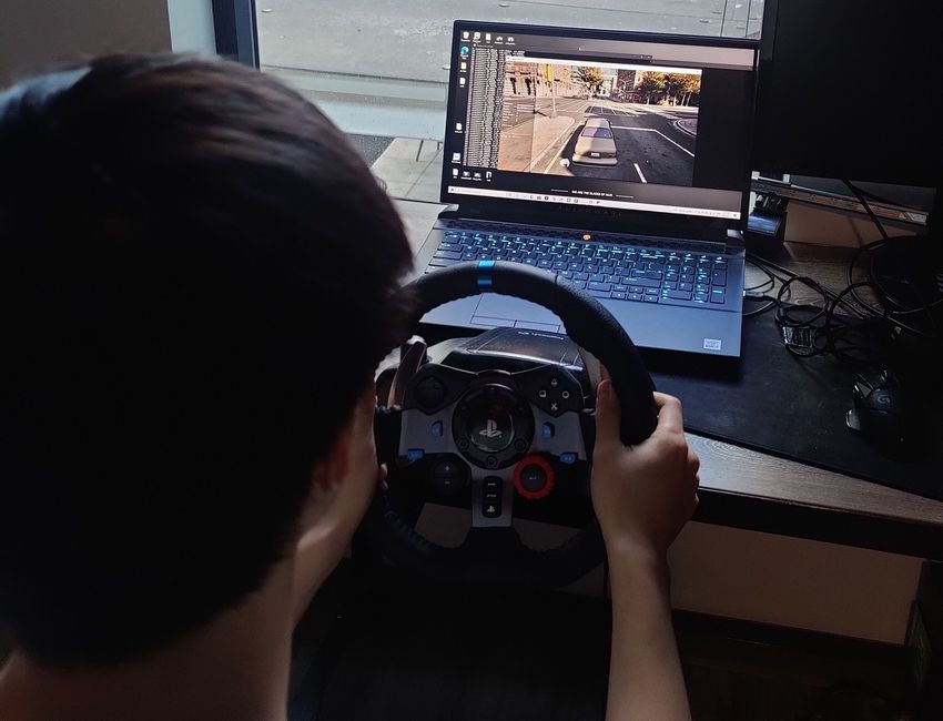
O NLINE N O - REGRET M ODEL -BASED M ETA RL FOR P ERSONALIZED NAVIGATION

    Next during the online phase when every iteration t a new M(t) comes in, at the beginning of
this iteration we first collect one trajectory τt with the exploration policy π e , then we perform one
shot adaptation on our latest meta model Pb(t) to obtain U (Pb(t) ), τt ):
                                                           X
                        U (Pb(t) , τt ) = Pb(t) + αadapt ∇     log(Pb(t) (s0 |s, a)).                (2)
                                                                s,a,s0 ∈τt

    After we have the estimation of the current dynamics, we can construct our policy π    b(t) , which
is defined by running model predictive control methods such as CEM De Boer et al. (2005), MPPI
Williams et al. (2017) or tree search Schrittwieser et al. (2020) on the current adapted dynamics
model U (Pb(t) , τt ). Thus we denote the policy as π
                                                    b(t) = MPC(U (Pb(t) , τt )).
    With the constructed policy π b , we then collect K trajectories inside the current M(t) : with
                                    (t)

probability 12 we will follow the current policy π   b(t) , and with probability 21 we will follow the
                        e 1
exploration policy π . For simplicity, we denote the state-action distribution induced by the
                                  e
exploration policy as νt := dπP (t) , which will be used for analysis in the next section. Finally
after we store all the trajectories we obtained in the current iteration into dataset Dt , along with
samples from previous iterations, we can perform no-regret online meta learning algorithm (e.g.,
Follow The Meta Leader) to obtain the new meta model Pb(t+1) :
                                                   t
                                                   X       X
                            Pb(t+1) = argmax                        log U (P, τn )(s0 |s, a).                          (3)
                                           P ∈P    n=1 s,a,s0 ∈Dn

Here we treat the model class and the meta model class as the same class since they are defined to
have the same parametrization.
     Thus the proposed method integrates online learning, meta learning and MBRL and is better
than the previous algorithms in the following sense: comparing with online SystemID methods,
our method can return a set of personalized policies when incoming environments have different
dynamics rather than policy for one fixed environment. Comparing with meta MBRL methods,
our method can learn to adapt in an online manner under extensive real-human user-study, where
previous methods only work in simulation. Also meta RL needs to be trained on a set of tasks before
testing so it is not applicable for our online setting. Another advantage of our method is that it has
theoretical guarantee comparing with the meta RL methods, which we will show in the next section.

5. Analysis
In this section we provide the regret analysis for Alg. 1. At a high level, our regret analysis is based
on the previous analysis of the online SystemID framework Ross and Bagnell (2012) that applies
DAgger Ross et al. (2011) in the MBRL setting to train the sequence of models, where DAgger can
be regarded as a no-regret online learning procedure such as Follow-the-Leader (FTL) algorithm
Shalev-Shwartz et al. (2011). In our setting, on the other hand, our model training framework could
be regarded as Follow-the-Meta-Leader (FTML) Finn et al. (2019) that is also no-regret with our
designed training objective. The overall intuition is that with the sequence of more reliable adapted
models, the regret can be bounded and diminish over time. We first introduce our assumptions:
 1. Note that the probability 21 here is for the ease of theoretical analysis. In fact, one can change the probability of
    rolling out with π e to arbitrary non-zero probability and will only change a constant coefficient on the final result.

                                                            5
O NLINE N O - REGRET M ODEL -BASED M ETA RL FOR P ERSONALIZED NAVIGATION
Assumption 1 (Optimal Control Oracle) We assume that the model predictive control methods
return us an − optimal policy. That is, for any transitional dynamics kernel P and initial state
distribution µ, we have
h i
Es∼µ V P,MPC(P ) (s) − min Es∼µ V P,π (s) ≤ oc .
π∈Π
Assumption 2 (Agnostic) We assume agnostic setting. That is, our model class may not contain
the ground truth meta model that can perfectly adapt to any dynamics. Formally, given arbitrary
state-action distribution d, one trajectory τ induced by P (t) , ∃Pb∗ ∈ P, such that ∀t ∈ [T ],
h i
Es,a∼d DKL (U (Pb∗ , τ )(·|s, a), P (t) (·|s, a)) ≤ model .
Note that oc and model are independent from our algorithm (i.e., we can not eliminate this term no
matter how carefully we design our algorithm).
Our analysis begins with bounding the performance difference between the sequence of policies
generated by our algorithm and any policy π 0 , which can be the policy induced by adapting from
the best meta-model. As the first step, we can relate the performance difference to the model error
with: 1. simulation lemma (Lemma 5) Kearns and Singh (2002); Sun et al. (2019). 2. We relate the
trajectories induced by π 0 and π e by the coefficient term introduced in the Sec. 3. Note that since we
should only care about comparing with “good” π 0 , the coefficient is small under such circumstances.
The next step is thus to bound the model error over the online process.
Let’s first observe the
following loss function: `(t) (P ) = Es,a∼ρt DKL P (·|s, a), P (t) (·|s, a) , where ρt defined as the
state-action distribution of our data collection scheme. This correspond
Pt to(t)the model error. Then if
we use FTML to update the meta model: P b (t+1) = argminP ∈P i=1 ` (U (P, τt )), it is easy to
see this update is equivalent to Eq. 3 as in our algorithm. Then we can invoke the main result from
Finn et al. (2019) (Lemma 8), and we are ready to present our main result:
Theorem 3 Let {Pb(t) }Tt=1 be the learned meta models. Let {U (Pb(t) , τt )}Tt=1 be the adapted model
after the one-shot adaptations. Let π b = {b b(t) := M P C(U (Pb(t) , τt )). Let ρt :=
π (t) }Tt=1 , where π
1 π (t) 1 (t)
2 dP (t) + 2 νt be the state-action distribution induced by our algorithm under M . Then for policy
b
0 0(t) T
sequence π = {π }t=1 , we have 2
π 0(t) )H 2
!
0(t) √ max(c
π ) − Jµ (π 0 ) ≤ oc + max(cπνt )H 2 model + Õ
Jµ (b √νt .
t T
We defer the full proofs in Appendix A. Thm. 3 shows that given any π 0 , which could be the policies
induced by the best meta model in the model class, the performance gap incurred by our algorithm
diminishes with rate Õ( √1T ), along with the inevitable terms oc and model , which our algorithm
has no control over. Since our main result is based on any arbitrary policy sequence, we here first
formally define the best adapted sequence of policies from hindsight, and we could easily conclude
with the no-regret conclusion in the following corollary:
2. Note that Õ hides the logarithmic terms.
6O NLINE N O - REGRET M ODEL -BASED M ETA RL FOR P ERSONALIZED NAVIGATION
Corollary 4 Let π π (t) }Tt=1 be the policies returned by our algorithm. Define πP∗ = argminπ∈Π
b = {b
Es∼µ V π,P ∗
(s). Let πP = {πU∗ (P,τt ) }Tt=1 . For simplicity let π ∗(t) = πU∗ (P,τt ) . Let R(T ) =
π ) − minP ∈P J(πP∗ ) be the regret of our algorithm. We have
J(b
∗(t) √
lim R(T ) = oc + max(cπνt )H 2 model .
T →∞ t
6. Experiments
6.1. System Setup
Our vehicle navigation system is developed inside the Carla simulator Dosovitskiy et al. (2017).
Each navigation run follows the below procedure: a vehicle spawns at a specified location inside
the simulator, and the navigation system provides one audio instruction to the user every one second
(45 frames). The user will control the vehicle with either a keyboard or a driving kit, and react to the
audio instructions, until the vehicle is near the specified destination point. The goal is to compare
the reliability of different navigation algorithms based on optimal path tracking and safety.
We develop the navigation system in 5 Carla native town maps, which include comprehensive
traffic situations. We use Carla’s built-in A* algorithm to search for the optimal path: we first
manually specify a starting point and destination point, which define a route, and the A* planner
returns a list of waypoints, defined by its x,y,z coordinates, that compose the optimal path.
To introduce various and comprehensive dynamics, we invite human participants with different
levels of skills and propose three ways to induce diverse dynamics: a) different built-in vehicles, b)
different visual conditions, c) different cameras (points of view), as shown in Fig. 2.
Finally, we introduce our design for the state and action spaces for our RL setting. We discretize
the system by setting every 45 frames (around 1s) as one time step. We design each route to have
a length of 2 minutes on average, thus each trajectory contains 120 state-action pairs on average.
Each state is a 14-dimensional vector that contains low-level information about the vehicle, user
inputs, and the immediate goal. For the action space, we adopt a discrete action space given
the limited audio generation and modification functionality of Carla’s interface. Nevertheless, we
observe that our current design suffices to deliver timely instructions combined with our proposed
algorithm. In fact, our algorithm could also expand the action space, which we will demonstrate in
detail in Sec 6.4. Concretely, one action corresponds to one audio instruction, and the action space
contains the 7 instructions in total, including the no instruction option. In practice, we only play
the corresponding audio when the current action is different from the previous action, or the current
action has been repeated for 15 timesteps.
We defer a complete list of system details in Appendix C: the town maps can be found in
Sec. C.1, state representation in Sec. C.2, actions in Sec. C.3, list of different vision conditions,
vehicles, driving kits in Sec. C.4.
6.2. Practical Implementation
In this section we introduce the practical implementation details. There are two major specifications
for a successful transfer from theory to practice: the model parametrization and the MPC method.
For the model parametrization, we represent the (meta) model class P as a class of deep
feedforward neural networks. Each element in the class can be denoted as Pθ , where here θ
is the parameters of P . Here we adopt a deterministic model given there is no stochasticity in
7O NLINE N O - REGRET M ODEL -BASED M ETA RL FOR P ERSONALIZED NAVIGATION
the underlying Carla system. Furthermore, since some instructions have lasting affect on system
dynamics (e.g., prepare to turn), we feed a history of state-action pairs to the network for robust
predictions. Concretely, the network input is a history of state-action pairs ht = {st−k , at−k }K k=0
and the output of the network is the predicted next state sbt+1 . In practice using K = 4 suffices
to include enough information for model prediction. In addition, we discover that predicting state
differences in the egocentric vehicle coordinates boosts the accuracy of the model.
Because of the deterministic system, maximizing log-likelihood is equivalent to minimizing
the l2 norms of the state differences. In this work, we follow the empirical success of L-step loss
Nagabandi et al. (2018b); Luo et al. (2018). Specifically, with a batch {ht , st+1 }B
t=1 , where B is the
batch size, for Pθ , we update the model by
B L
!
X X
θ := θ − αmeta ∇θ k(ŝi+l − ŝi+l−1 ) − (si+l − si+l−1 )k2 , (4)
i=1 l=1
where ĥi = hi and ŝi+l+1 = U (Pθ (ĥi+l , ai+l )), and ĥi+l+1 is constructed by discarded the first
state action pair in ĥi+l+1 and concatenate ŝi+l+1 and ai+l+1 to its end. In our experiments, we use
L = 5. Similarly, the parameter of U (Pθ ) is obtained by using Eq. 4 with the adaptation sample
(line 3 in Alg. 1) where next states are predicted by Pθ .
For MPC, since the action space is discrete, we adopt a tree search scheme, although the
current design can be easily switched to MPPI
PH or CEM. We define the cost of an action sequence
{ah }Hh=1 under P θ by: C({a } H ,P ) =
h h=1 θ h=1 kŝh+1 −g k
h+1 2
2 , where {ŝ H
h+1 }h=1 are obtained by
autoregressively rolling out Pθ with {ah }H H
h=1 and {gh+1 }h=1 are the coordinates of goal waypoints.
Note on the right hand side we abuse notation by letting ŝ also be coordinates (but not the full states).
Intuitively, we want the model-induced policy to be a residual policy of the explore policy, since
the explore policy is accurate (but not personalized enough) for most situations. Thus we reward
an action sequence that is the same as the explore policy action sequence (but at potentially shifted
time intervals). We also add penalties for turning actions where there are no junctions.
6.3. Experimental Results
We evaluate our practical algorithm inside the system described in Sec. 6.1. For each of the 5 towns,
we design 10 routes that contain all traffic conditions. We define using one navigation algorithm
to run the 10 routes in one town as one iteration. For each of the towns, we first use the explore
policy to collect 3 iterations of samples as the offline dataset. For the online process, the first 7
iterations involve different vehicles and visual conditions. In 3 out of 5 towns, we invite additional
6 participants with diverse driving skills to complete the next 6 iterations. Then for all the maps,
we include 2 additional iterations that are controlled by different control equipment. Each human
participant contributes at least 3-hour driving inside the system, and in total more than 60-hour
driving data is used for our final evaluation.
We include three baselines in this study: the first is the explore policy3 , a non-learning-based
policy based on A* path planning algorithm. The underlying backbone of the explore policy is the
Carla’s autopilot agent, which provides expert demonstrations for the state-of-the-art autonomous
3. The name “explore policy” inherits from Ross and Bagnell (2012), but here the explore policy is actually a very
strong baseline, as described in the main text.
8O NLINE N O - REGRET M ODEL -BASED M ETA RL FOR P ERSONALIZED NAVIGATION
Town1 Town2 Town3
170
Explore
Average Episodic Costs
Average Episodic Costs
Average Episodic Costs
160 SysID (Ross and Bagnell 2012)
140 180
Adapt (Ours)
150 Adapt_speed (Ours)
130 160
140
130 120 140
120
110 120
110
100 100 100
0 1 2 3 4 5 6 7 8 9 10 11 12 13 14 0 1 2 3 4 5 6 7 8 9 10 11 12 13 14 0 1 2 3 4 5 6 7 8 9 10 11 12 13 14
Users/Iterations Users/Iterations Users/Iterations
Figure 3: Performance bar plots of the four baselines in three town maps. The metric we use is the average
episodic accumulative costs upon the current iteration. Here the episodic accumulative costs are calculated
by averaging the point-wise tracking error over the ten routes that we defined in Sec. 6.1
driving algorithms Chen et al. (2020b, 2021b); Prakash et al. (2021). To increase the accuracy and
robustness of the policy, we further include hard-coded heuristics for the corner cases. The second
baseline is a policy induced by the non-adaptive model trained online Ross and Bagnell (2012).
We refer to this policy as SysID in the rest of the sections. The model training of SysID follows
Eq. 4 with only one exception that the next states are predicted directly by the models instead of
the adapted models (i.e., no meta adaptation). The third baseline is our algorithm and we include a
variation of our algorithm as well, which will be introduced in detail in Sec. 6.4.
The metric we use in this section is the point-wise tracking error. Concretely, for a state st , the
cost we are evaluating is c(st ) = kxst − xgt−1 , yst − ygt−1 k22 , where x, y denotes the coordinates
elements inside a state and gt−1 denotes the goal selected from the waypoint list from the last
(t)
ˆ = T1 Tt=1 Htπ , where Ht
P
timestep. We follow Sec. 3 and plot the empirical performance J(π)
is the sum of costs in one episode. We show the performance of the 4 baselines in 3 town maps
that involve human participants with different levels of driving skills in Fig. 3 (we defer the results
of the remaining two maps in Appendix D). We observe that except for the first online iteration,
our method (denoted as adapt) beats the other two baselines (explore and SysID) consistently
in tracking the optimal routes. There are two possible reasons that the navigation system could
accumulate huge costs: an ill-timed instruction could cause the drive to miss a turn at a junction
thus follow a suboptimal route. On the other hand, if the navigation system is not adaptive to the
driver, mildly ill-timed instructions may still keep the driver on the optimal route, but deviate from
the waypoints (e.g., driving on the sidewalk). This will also raise safety issues as we will further
evaluate in Sec. 6.5. Note that our results indicate the significance of personalization: non-adaptive
methods, even with online updates (SysID), behave suboptimally and we observe the performance
gaps between non-adaptive methods and our method increase as the more users are involved in the
system. We also observe that dynamics change induced by different users is much more challenging
than simulation-based dynamics change as real human participants introduce significantly greater
dynamics shifts than simulation-based changes, as indicated in Fig.3 starting from user/iteration 7.
6.4. Generating New Actions
In this section we analyze a new variant of our adaptive policy: adaptive policy with speed change.
The new policy is designed to generate new actions by changing the playback speed of the original
instructions: slower, normal and faster. Thus the new policy increases the action space dimensions
by three times. We include the performance of this new variant along with other baselines in
9O NLINE N O - REGRET M ODEL -BASED M ETA RL FOR P ERSONALIZED NAVIGATION
Fig. 3, denoted as “Adaptive speed”. We see that this new policy design performs similarly to
the original adaptive policy at the first few iterations due to the lack of samples with speed change,
but it gradually outperforms as the online procedure goes on.
6.5. Safety
In addition to better tracking, our empirical evaluation also shows that our method has better safety
guarantees. In this section, we present the number of collisions for each method in Table 1. In each
cell we show the total number of collisions averaged over the 10 routes in the corresponding town
maps. We then average over the 15 online iterations and present the mean and standard deviation.
We observe that comparing with the explore policy baseline, our methods (adaptive and adaptive
speed) achieve over 50% and 60% decrease in terms of the number of collisions, respectively. The
results indicate that by better tracking the optimal path and delivering more timely instructions with
personalized policies, the adaptive policies indeed achieve a stronger safety guarantee.
6.6. Empirical Regret
In this section, we analyze the empirical regret of the adaptive policy, i.e., how our adaptive policy
compares with the policy induced by the best empirical meta model from hindsight. We train the
hindsight policy using the data collected from all 15 iterations and train with Eq. 3. We compare the
two policies in Fig. 4, following the same metric as in Fig. 3. The results show that the performance
gap exists at the beginning, but it closes up as the online process proceeds. Here we want to
emphasize that in practice, this empirical regret (performance gap) may not diminish strictly at
a rate of T −1/2 since we could only expect such rate in expectation, we do observe that such gap
decreases over time and in some iteration, the performance of the adaptive policy is actually the
same as the best policy from hindsight, indicating the strong adaptability of our proposed method.
Town2 Town2
Average Episodic Costs
Adapt (Ours) Regret
125 Best_hindsight 12 Town1 Town2 Town3
120
10 Explore policy 3.08 (1.73) 1.00 (1.18) 1.38 (1.21)
115
Regret
110 8
105 SysID 2.23 (1.19) 0.69 (1.14) 1.23 (1.19)
6
100
95 4
Adapt (Ours) 1.85 (1.29) 0.31 (0.61) 0.69 (0.72)
90
0 7 14 0 7 14 Adapt Speed (Ours) 1.54 (1.45) 0.23 (0.42) 0.54 (0.50)
Iterations/Users Iterations/Users
Figure 4: Evaluation of empirical Table 1: Average counts of total collisions of each
regret/performance gap of the adaptive baseline in the 3 town maps. The average is over 15 online
policy in town 2. The evaluation metric and iterations and the standard deviation is indicated in the
presentation follow Fig. 3. parenthesis.
7. Summary
In this work we propose an online meta MBRL algorithm that can adapt to different incoming
dynamics in an online fashion. We proved that our algorithm is no-regret. We specifically study
the application of the proposed algorithm in personalized voice navigation and develop a machine
learning system, which could also be beneficial for future research. The extensive real-world use
study shows that our algorithm could indeed efficiently adapt to unseen dynamics, and also improve
the safety of the voice navigation.
10O NLINE N O - REGRET M ODEL -BASED M ETA RL FOR P ERSONALIZED NAVIGATION
References
Suneel Belkhale, Rachel Li, Gregory Kahn, Rowan McAllister, Roberto Calandra, and Sergey
Levine. Model-based meta-reinforcement learning for flight with suspended payloads. IEEE
Robotics and Automation Letters, 6(2):1471–1478, 2021.
Changan Chen, Unnat Jain, Carl Schissler, Sebastia Vicenc Amengual Gari, Ziad Al-Halah,
Vamsi Krishna Ithapu, Philip Robinson, and Kristen Grauman. Soundspaces: Audio-visual
navigation in 3d environments. In Computer Vision–ECCV 2020: 16th European Conference,
Glasgow, UK, August 23–28, 2020, Proceedings, Part VI 16, pages 17–36. Springer, 2020a.
Changan Chen, Sagnik Majumder, Ziad Al-Halah, Ruohan Gao, Santhosh Kumar Ramakrishnan,
and Kristen Grauman. Learning to set waypoints for audio-visual navigation. arXiv preprint
arXiv:2008.09622, 2020b.
Changan Chen, Ziad Al-Halah, and Kristen Grauman. Semantic audio-visual navigation. In
Proceedings of the IEEE/CVF Conference on Computer Vision and Pattern Recognition, pages
15516–15525, 2021a.
Dian Chen, Vladlen Koltun, and Philipp Krähenbühl. Learning to drive from a world on rails. arXiv
preprint arXiv:2105.00636, 2021b.
Kurtland Chua, Roberto Calandra, Rowan McAllister, and Sergey Levine. Deep reinforcement
learning in a handful of trials using probabilistic dynamics models. In Advances in Neural
Information Processing Systems, pages 4754–4765, 2018.
Ignasi Clavera, Jonas Rothfuss, John Schulman, Yasuhiro Fujita, Tamim Asfour, and Pieter Abbeel.
Model-based reinforcement learning via meta-policy optimization. In Conference on Robot
Learning, pages 617–629. PMLR, 2018.
Andrea F Daniele, Mohit Bansal, and Matthew R Walter. Navigational instruction generation
as inverse reinforcement learning with neural machine translation. In 2017 12th ACM/IEEE
International Conference on Human-Robot Interaction (HRI, pages 109–118. IEEE, 2017.
Pieter-Tjerk De Boer, Dirk P Kroese, Shie Mannor, and Reuven Y Rubinstein. A tutorial on the
cross-entropy method. Annals of operations research, 134(1):19–67, 2005.
Niranjan Deshpande and Anne Spalanzani. Deep reinforcement learning based vehicle navigation
amongst pedestrians using a grid-based state representation. In 2019 IEEE Intelligent
Transportation Systems Conference (ITSC), pages 2081–2086. IEEE, 2019.
Alexey Dosovitskiy, German Ros, Felipe Codevilla, Antonio Lopez, and Vladlen Koltun. Carla: An
open urban driving simulator. In Conference on robot learning, pages 1–16. PMLR, 2017.
Yan Duan, John Schulman, Xi Chen, Peter L Bartlett, Ilya Sutskever, and Pieter Abbeel. Rl 2 : Fast
reinforcement learning via slow reinforcement learning. arXiv preprint arXiv:1611.02779, 2016.
Chelsea Finn, Pieter Abbeel, and Sergey Levine. Model-agnostic meta-learning for fast adaptation
of deep networks. In International Conference on Machine Learning, pages 1126–1135. PMLR,
2017a.
11O NLINE N O - REGRET M ODEL -BASED M ETA RL FOR P ERSONALIZED NAVIGATION
Chelsea Finn, Tianhe Yu, Tianhao Zhang, Pieter Abbeel, and Sergey Levine. One-shot visual
imitation learning via meta-learning. In Conference on Robot Learning, pages 357–368. PMLR,
2017b.
Chelsea Finn, Aravind Rajeswaran, Sham Kakade, and Sergey Levine. Online meta-learning. In
International Conference on Machine Learning, pages 1920–1930. PMLR, 2019.
Jacaueline Hemminahaus and Stefan Kopp. Towards adaptive social behavior generation for
assistive robots using reinforcement learning. In 2017 12th ACM/IEEE International Conference
on Human-Robot Interaction (HRI, pages 332–340. IEEE, 2017.
Tariq Iqbal, Maryam Moosaei, and Laurel D Riek. Tempo adaptation and anticipation methods for
human-robot teams. In RSS, Planning HRI: Shared Autonomy Collab. Robot. Workshop, 2016.
Gregory Kahn, Adam Villaflor, Bosen Ding, Pieter Abbeel, and Sergey Levine. Self-supervised
deep reinforcement learning with generalized computation graphs for robot navigation. In 2018
IEEE International Conference on Robotics and Automation (ICRA), pages 5129–5136. IEEE,
2018.
Michael Kearns and Satinder Singh. Near-optimal reinforcement learning in polynomial time.
Machine learning, 49(2):209–232, 2002.
B Ravi Kiran, Ibrahim Sobh, Victor Talpaert, Patrick Mannion, Ahmad A Al Sallab, Senthil
Yogamani, and Patrick Pérez. Deep reinforcement learning for autonomous driving: A survey.
IEEE Transactions on Intelligent Transportation Systems, 2021.
Songsang Koh, Bo Zhou, Hui Fang, Po Yang, Zaili Yang, Qiang Yang, Lin Guan, and Zhigang Ji.
Real-time deep reinforcement learning based vehicle navigation. Applied Soft Computing, 96:
106694, 2020.
Zichuan Lin, Garrett Thomas, Guangwen Yang, and Tengyu Ma. Model-based adversarial meta-
reinforcement learning. arXiv preprint arXiv:2006.08875, 2020.
Lucia Liu, Daniel Dugas, Gianluca Cesari, Roland Siegwart, and Renaud Dubé. Robot navigation
in crowded environments using deep reinforcement learning. In 2020 IEEE/RSJ International
Conference on Intelligent Robots and Systems (IROS), pages 5671–5677. IEEE, 2020.
Yuping Luo, Huazhe Xu, Yuanzhi Li, Yuandong Tian, Trevor Darrell, and Tengyu Ma. Algorithmic
framework for model-based deep reinforcement learning with theoretical guarantees. arXiv
preprint arXiv:1807.03858, 2018.
Anusha Nagabandi, Ignasi Clavera, Simin Liu, Ronald S Fearing, Pieter Abbeel, Sergey Levine,
and Chelsea Finn. Learning to adapt in dynamic, real-world environments through meta-
reinforcement learning. arXiv preprint arXiv:1803.11347, 2018a.
Anusha Nagabandi, Chelsea Finn, and Sergey Levine. Deep online learning via meta-learning:
Continual adaptation for model-based rl. arXiv preprint arXiv:1812.07671, 2018b.
Eshed OhnBar, Kris Kitani, and Chieko Asakawa. Personalized dynamics models for adaptive
assistive navigation systems. In Conference on Robot Learning, pages 16–39. PMLR, 2018.
12O NLINE N O - REGRET M ODEL -BASED M ETA RL FOR P ERSONALIZED NAVIGATION
Aditya Prakash, Kashyap Chitta, and Andreas Geiger. Multi-modal fusion transformer for end-to-
end autonomous driving. In Proceedings of the IEEE/CVF Conference on Computer Vision and
Pattern Recognition, pages 7077–7087, 2021.
Stephane Ross and J Andrew Bagnell. Agnostic system identification for model-based
reinforcement learning. arXiv preprint arXiv:1203.1007, 2012.
Stephane Ross, Brahim Chaib-draa, and Joelle Pineau. Bayesian reinforcement learning in
continuous pomdps with application to robot navigation. In 2008 IEEE International Conference
on Robotics and Automation, pages 2845–2851. IEEE, 2008.
Stéphane Ross, Geoffrey Gordon, and Drew Bagnell. A reduction of imitation learning and
structured prediction to no-regret online learning. In Proceedings of the fourteenth international
conference on artificial intelligence and statistics, pages 627–635. JMLR Workshop and
Conference Proceedings, 2011.
Steindór Sæmundsson, Katja Hofmann, and Marc Peter Deisenroth. Meta reinforcement learning
with latent variable gaussian processes. arXiv preprint arXiv:1803.07551, 2018.
Julian Schrittwieser, Ioannis Antonoglou, Thomas Hubert, Karen Simonyan, Laurent Sifre, Simon
Schmitt, Arthur Guez, Edward Lockhart, Demis Hassabis, Thore Graepel, et al. Mastering atari,
go, chess and shogi by planning with a learned model. Nature, 588(7839):604–609, 2020.
Shai Shalev-Shwartz et al. Online learning and online convex optimization. Foundations and trends
in Machine Learning, 4(2):107–194, 2011.
Yuda Song and Wen Sun. Pc-mlp: Model-based reinforcement learning with policy cover guided
exploration. In International Conference on Machine Learning, pages 9801–9811. PMLR, 2021.
Andreas Stafylopatis and Konstantinos Blekas. Autonomous vehicle navigation using evolutionary
reinforcement learning. European Journal of Operational Research, 108(2):306–318, 1998.
Wen Sun, Nan Jiang, Akshay Krishnamurthy, Alekh Agarwal, and John Langford. Model-based
rl in contextual decision processes: Pac bounds and exponential improvements over model-free
approaches. In Conference on learning theory, pages 2898–2933. PMLR, 2019.
Hartmut Surmann, Christian Jestel, Robin Marchel, Franziska Musberg, Houssem Elhadj, and
Mahbube Ardani. Deep reinforcement learning for real autonomous mobile robot navigation
in indoor environments. arXiv preprint arXiv:2005.13857, 2020.
Richard S Sutton and Andrew G Barto. Reinforcement learning: An introduction. MIT press, 2018.
Andrea Lockerd Thomaz, Cynthia Breazeal, et al. Reinforcement learning with human teachers:
Evidence of feedback and guidance with implications for learning performance. In Aaai,
volume 6, pages 1000–1005. Boston, MA, 2006.
Cristen Torrey, Susan R Fussell, and Sara Kiesler. How a robot should give advice. In 2013 8th
ACM/IEEE International Conference on Human-Robot Interaction (HRI), pages 275–282. IEEE,
2013.
13O NLINE N O - REGRET M ODEL -BASED M ETA RL FOR P ERSONALIZED NAVIGATION
Stephen Tu and Benjamin Recht. The gap between model-based and model-free methods on the
linear quadratic regulator: An asymptotic viewpoint. In Conference on Learning Theory, pages
3036–3083. PMLR, 2019.
Tingwu Wang, Xuchan Bao, Ignasi Clavera, Jerrick Hoang, Yeming Wen, Eric Langlois,
Shunshi Zhang, Guodong Zhang, Pieter Abbeel, and Jimmy Ba. Benchmarking model-based
reinforcement learning. CoRR, abs/1907.02057, 2019. URL http://arxiv.org/abs/
1907.02057.
Yi Wang, Manfred Huber, Vinay N Papudesi, and Diane J Cook. User-guided reinforcement
learning of robot assistive tasks for an intelligent environment. In Proceedings 2003 IEEE/RSJ
International Conference on Intelligent Robots and Systems (IROS 2003)(Cat. No. 03CH37453),
volume 1, pages 424–429. IEEE, 2003.
Grady Williams, Nolan Wagener, Brian Goldfain, Paul Drews, James M Rehg, Byron Boots, and
Evangelos A Theodorou. Information theoretic mpc for model-based reinforcement learning.
In 2017 IEEE International Conference on Robotics and Automation (ICRA), pages 1714–1721.
IEEE, 2017.
14O NLINE N O - REGRET M ODEL -BASED M ETA RL FOR P ERSONALIZED NAVIGATION
Appendix A. Proofs
In this section we prove Thm. 3. We first introduce the simulation lemma:
Lemma 5 (Simulation Lemma) Consider two MDPs M1 = {C, P } and 0 0
π,P,c
M2 = {C , P } where
C and P represent cost and transition. Let J(π; C, P ) = Es∼µ V (s) , where the superscript C
denotes that the value function V is the expected sum of cost C, and for simplicity let V π = V π,P,C .
Then for any policy π : S × A 7→ ∆(A), we have:
H−1
X
0 0
Es,a∼dπh C(s, a) − C 0 (s, a) + Es0 ∼P (·|s,a) Vhπ (s0 ) − Es0 ∼P 0 (·|s,a) Vhπ (s0 ) .
J(π; C, P ) − J(π; C , P ) =
h=0
We omit the proof since the simulation lemma is widely used in MBRL analysis. We refer the reader
to lemma 10 of Sun et al. (2019) for an example.
Then let’s start off with an easier problem, where we bound the performance difference between
two single policies:
b, π 0 ∈ Π, where Pb ∈ P and π
Lemma 6 Let π b = M P C(Pb). Let ν be an exploration distribution,
we have:
0
h i
π ) − Jµ (π 0 ) ≤ oc + H 2 (cπb + cπ )Es,a∼ν kPb(·|s, a) − P (·|s, a)k1
Jµ (b ν ν
Proof For simplicity, denote Vb π = V π,P , we have
b
0
π ) − Jµ (π 0 ) = Es∼µ [V πb (s) − V π (s)]
Jµ (b
0 0 0
= Es∼µ [V πb (s) − Vb πb (s)] + Es∼µ [Vb πb (s) − Vb π (s)] + Es∼µ [Vb π (s) − V π (s)]
0 0 0 0
= Es∼µ [Vb πb (s) − Vb π (s)] + Es∼µ [V π (s) − Vb πb (s)] + Es∼µ [Vb π (s) − V π (s)]
H−1
X h i
≤ oc + Es,a∼dπb Es0 ∼Pb(·|s,a) Vbhπb (s0 ) − Es0 ∼P (·|s,a) Vbhπb (s0 )
h
h=0
H−1 h i
0 0
X
+ Es,a∼dπb Es0 ∼Pb(·|s,a) Vbhπ (s0 ) − Es0 ∼P (·|s,a) Vbhπ (s0 )
h
h=0
H−1 h i
0 0 0
X
≤ oc + (cπνb + cπν ) Es,a∼ν Es0 ∼Pb(·|s,a) Vbhπ (s0 ) − Es0 ∼P (·|s,a) Vbhπ (s0 )
h=0
H−1 h i
0 0
X
≤ oc + (cπνb + cπν ) Es,a∼ν kPb(·|s, a) − P (·|s, a)k1 kVbhπ k∞
h=0
0
h i
2
≤ oc + H (cπνb + cνπ )Es,a∼ν kPb(·|s, a) − P (·|s, a)k1
The first inequality is by simulation lemma, the second is by the definition of the coverage coefficient,
and the third is by Holder’s inequality, and the last is by the assumption that the costs are bounded
by 1.
With the previous lemma, we are ready to prove Lemma 7:
15O NLINE N O - REGRET M ODEL -BASED M ETA RL FOR P ERSONALIZED NAVIGATION
Lemma 7 Let {Pb(t) }Tt=1 be the learned meta models. Let {U (Pb(t) , τt )}Tt=1 be the adapted model
after the one-shot adaptations. Let π b = {b π (t) }Tt=1 , where π
b(t) := M P C(Ut (Pb(t) )). Let ρt :=
1 π (t) 1 (t)
2 dP (t) + 2 νt be the state-action distribution induced by our algorithm under M . Then for policy
b
sequence π 0 = {π 0(t) }Tt=1 , we have:
T
0(t) 1X
π ) − Jµ (π 0 ) ≤ oc + 2 max(cπνi )H 2
Jµ (b Es,a∼ρt kU (Pb(t) , τt )(·|s, a) − P (t) (·|s, a)k1
t T
t=1
Proof
T
1 X
π ) − Jµ (π 0 ) =
Jµ (b π (t) ) − Jµ (π 0(t) )
Jµ (b
T
t=1
T H−1
HXX h
b(t) , τt )(·|s, a) − P (t) (·|s, a)k1
i
≤ oc + E (t) kU ( P
T s,a∼dπ b
t=1 h=0 h,P (t)
h i
(t) (t)
+ Es,a∼dπ 0 kU (P , τt )(·|s, a) − P (·|s, a)k1
b
h,P (t)
T H−1
HXX h
b(t) , τt )(·|s, a) − P (t) (·|s, a)k1
i
≤ oc + E (t) kU ( P
T s,a∼dπ
b
t=1 h=0 h,P (t)
h i
π 0(t) (t) (t)
+ cνt Es,a∼νt kU (P , τt )(·|s, a) − P (·|s, a)k1
b
T H−1
H X X π0(t) h
(t) (t)
i
≤ oc + cνt E b (t) kU (Pb , τt )(·|s, a) − P (·|s, a)k1
T s,a∼dπ
t=1 h=0 h,P (t)
h i
π 0(t) (t) (t)
+ cνt Es,a∼νt kU (P , τt )(·|s, a) − P (·|s, a)k1
b
T H−1
2H 2 X π0(t) X 1 h i
= oc + cνt E π (t) kU (Pb(t) , τt )(·|s, a) − P (t) (·|s, a)k1
T 2H s,a∼dh,P (t)
b
t=1 h=0
1 h i
(t) (t)
+ Es,a∼νt kU (Pb , τt )(·|s, a) − P (·|s, a)k1
2H
T
2H 2 X π0(t)
h i
(t) (t)
= oc + cνt Es,a∼ρt kU (P , τt )(·|s, a) − P (·|s, a)k1
b
T
t=1
0(t) T
2 maxt (cπνt )H 2 X h i
≤ oc + Es,a∼ρt kU (Pb(t) , τt )(·|s, a) − P (t) (·|s, a)k1
T
t=1
16O NLINE N O - REGRET M ODEL -BASED M ETA RL FOR P ERSONALIZED NAVIGATION
Lemma 8 (Regret bound of FTML) Suppose that `(t) are strongly convex. With αadapt and αmeta
properly chosen, FTML has the regret
T
X T
X
RF T M L (T ) = `(t) (U (Pb(t) , τt )) − min `(t) (U (P, τt )) ≤ O(log(T )).
P ∈P
t=1 t=1
For proof we refer the reader to Finn et al. (2019).
The final step left to prove the main theorem remains to bound the model error. With the above
lemma, we show another lemma that leads to the main result:
(t)
Lemma 9 Let π b(t) := M P C U (Pb(t) , τt ) . Let ρt := 12 dπPb (t) + 12 νt be the state-action distribution
induced by our algorithm under M(t) . We have
T
1X h i 1
Es,a∼ρt kU (Pb(t) , τt )(·|s, a) − P (t) (·|s, a)k1 ≤ Õ √ .
T T
t=1
Proof Let the loss function `(t) be
h i
`(t) (P ) = Es,a∼ρt Es0 ∼P (t) (·|s,a) − log(P (s0 |s, a)) .
Since {Pb(t) }Tt=1 is obtained by running FTML on the sequence of strongly convex function {`(t) }Tt=1 ,
we have by Lemma 8 that
T
X T
X
(t) (t)
` U (P , τt ) ≤ min
b `(t) U (Pb(t) , τt ) + O(log(T ))
P ∈P
t=1 t=1
T
X T
X
`(t) U (Pb(t) , τt ) + Es,a∼ρt Es0 ∼P (·|s,a) log(P (t) (s0 |s, a)) ≤ min `(t) U (Pb(t) , τt )
P ∈P
t=1 t=1
+ Es,a∼ρt Es0 ∼P (·|s,a) log(P (t) (s0 |s, a)) + O(log(T )
T
X T
X
(t) (t)
Es,a∼ρt DKL U (P , τt )(·|s, a), P (·|s, a) ≤ min
b Es,a∼ρt DKL U (P, τt )(·|s, a), P (t) (·|s, a)
P ∈P
t=1 t=1
+ O(log(T ))
T
X
Es,a∼ρt DKL U (Pb(t) , τt )(·|s, a), P (t) (·|s, a) ≤ T model + O(log(T )),
t=1
where the last line is obtained by Assumption 2.
17O NLINE N O - REGRET M ODEL -BASED M ETA RL FOR P ERSONALIZED NAVIGATION
Finally by Pinsker’s inequality and Jensen’s inequality,
T T r
1X h
(t) 0 (t) 0
i 1 X
Es,a∼ρt Es0 ∼P (·|s,a) kU (Pb , τt )(s |s, a) − P (s |s, a)k1 ≤ 2Es,a∼ρt DKL U (Pb(t) , τt ), P (t)
T T
t=1 t=1
v
u
u1 X T
≤t 2Es,a∼ρt DKL U (Pb(t) , τt ), P (t)
T
t=1
√ 1
≤ model + Õ √ .
T
Then apply Lemma 9 on Lemma 7, we obtain our main theorem:
Theorem 10 (Main Theorem) Let {Pb(t) }Tt=1 be the learned meta models. Let {U (Pb(t) , τt )}Tt=1 be
the adapted model after the one-shot adaptations. Let π b = {bπ (t) }Tt=1 , where π
b(t) := M P C(Ut (Pb(t) )).
(t)
Let ρt := 21 dPπb (t) + 12 νt be the state-action distribution induced by our algorithm under M(t) . Then
for any meta policy π 0 , we have:
0(t)
!
0 π 0(t) 2√ maxt (cνπt )H 2
Jµ (b π ) − Jµ (π ) ≤ oc + max(cνt )H model + Õ √
t T
Proof This is a direct combination of Lemma 7 and Lemma 9.
Finally we can use our main theorem to reach the no-regret conclusion:
b = {b
Corollary 11 Let π π (t) }Tt=1 be the policies returned by our algorithm. Let R(T ) = J(b
π) −
∗
minπ∗ ∈Π J(π ) be the regret of our algorithm. We have
∗(t) √
lim R(T ) = oc + max(cπνt )H 2 model .
T →∞ t
Proof Let π ∗ = minπ∗ ∈Π J(π ∗ ). Replace π 0 by π ∗ in Thm. 3 we have
∗(t)
!
∗(t) √ maxt (cπνt )H 2
R(T ) = oc + max(cπνt )H 2 model + Õ √ .
t T
Taking T → ∞ completes the proof.
18O NLINE N O - REGRET M ODEL -BASED M ETA RL FOR P ERSONALIZED NAVIGATION
Appendix B. Algorithm
In this section, we provide the pseudocode of our algorithm.
Algorithm 1 Online Meta Model Based RL
Require: exploration policy π e , offline data Doff
1: Get warm-started model P b(1) with Eq.1
2: for t = 1, . . . , T do
3: Collect one trajectory τt = {sh , ah , sh+1 |ah ∼ π e , sh+1 ∼ P (t) (sh , ah )}H
h=1
4: Get U (Pb(t) , τt ) with Eq. 2.
5: b(t) ←
π − MPC U (Pb(t) , τt )
6: Dt = {}
7: for k = 1, . . . , K do
8: With prob. 12 rollout using current policy π b(t) :
9: τk = {sh , ah , sh+1 |ah ∼ π b , sh+1 ∼ P (·|sh , ah )}H
(t) (t)
h=1
10: Otherwise rollout using exploration policy π e :
11: τk = {sh , ah , sh+1 |ah ∼ π e , sh+1 ∼ P (t) (·|sh , ah )}H
h=1
12: Dt ←− Dt ∪ τk .
13: end for
14: Get Pb(t+1) by Eq. 3.
15: end for
19O NLINE N O - REGRET M ODEL -BASED M ETA RL FOR P ERSONALIZED NAVIGATION
Appendix C. System Details
C.1. Town maps
In this section, we show the town maps that are used in the development of our system in Fig. 5.
Figure 5: From left to right: the maps of Town1, Town2, Town3, Town4 and Town5 in our experiments.
C.2. State Representation
In this section, we describe the details of our state representation in our navigation system. At each
time step, the state is a concatenation of the following attributes:
• the current (x,y,z) coordinates of the vehicle.
• The current velocity in the x,y,z direction.
• The current heading (in radius) of the vehicle.
• An indicator i = e−d , where d is the distance to the next junction along the route.
• A boolean indicating whether the vehicle is at a roundabout.
• The (x,y) coordinates of the next waypoint in the route list return by the A* planner, which is
selected according to the current speed of the vehicle.
• The steering input from the user.
• A boolean indicating whether the vehicle is in reverse mode.
• The braking input from the user.
C.3. List of instructions
• No instruction.
• Turn left.
• Turn right.
• Prepare to turn left.
• Prepare to turn right.
• Enter the roundabout.
• Keep left (in the roundabout).
20O NLINE N O - REGRET M ODEL -BASED M ETA RL FOR P ERSONALIZED NAVIGATION
C.4. Iteration Details
In this section, we introduce the environment (user, vehicle, visual condition, etc.) involved in each
iteration in Table 2.
Iteration User Vehicle Camera Visual Control
index Index Condition Equipment
Offline 0 1 Chevrolet Camaro First personal view Normal Keyboard
Offline 1 1 Chevrolet Camaro Third personal view Normal Keyboard
Offline 2 1 Tesla Cybertruck First personal view Normal Keyboard
Online 0 1 Tesla Cybertruck Third personal view Normal Keyboard
Online 1 1 Chevrolet Camaro First personal view RGB Keyboard
Online 2 1 Chevrolet Camaro Third personal view Foggy Keyboard
Online 3 1 Chevrolet Camaro First personal view Foggy Keyboard
Online 4 1 Tesla Cybertruck Third personal view Foggy Keyboard
Online 5 1 Tesla Cybertruck First personal view Foggy Keyboard
Online 6 1 Tesla Cybertruck Top view Foggy Keyboard
Online 7 2 Chevrolet Camaro Third personal view Normal Keyboard
Online 8 3 Chevrolet Camaro Third personal view Normal Keyboard
Online 9 4 Chevrolet Camaro Third personal view Normal Keyboard
Online 10 5 Chevrolet Camaro Third personal view Normal Keyboard
Online 11 6 Chevrolet Camaro Third personal view Normal Keyboard
Online 12 7 Chevrolet Camaro Third personal view Normal Keyboard
Online 13 1 Chevrolet Camaro First personal view Normal Logitech G29
Online 14 1 Chevrolet Camaro Third personal view Normal Logitech G29
Table 2
21O NLINE N O - REGRET M ODEL -BASED M ETA RL FOR P ERSONALIZED NAVIGATION
Appendix D. Additional Experiments
In this section, we provide results from the two remaining town maps. The evaluations are the same
as in Sec. 6.3 and Sec. 6.5. We observe that the results from the additional experiments follow the
trend in Sec. 6.3 and Sec. 6.5.
D.1. Tracking Error
Town4 Town5
260
Explore Explore
Average Episodic Costs
Average Episodic Costs
SysID (Ross and Bagnell 2012) 110 SysID (Ross and Bagnell 2012)
240 Adapt (Ours) Adapt (Ours)
Adapt_speed (Ours) Adapt_speed (Ours)
220 100
200 90
180
80
160
70
0 1 2 3 4 5 6 7 8 0 1 2 3 4 5 6 7 8
Users/Iterations Users/Iterations
Figure 6: Performance bar plots of the four baselines in the remaining two town maps. The metric we use is
the average episodic accumulative costs upon the current iteration. Here the episodic accumulative costs are
calculated by averaging the point-wise tracking error over the ten routes that we defined in Sec. 6.1
D.2. Safety
Town4 Town5
Explore policy 4.00 (0.67) 2.89 (0.99)
SysID (Ross and Bagnell 2012) 3.00 (0.82) 2.11 (0.74)
Adaptive (Ours) 2.22 (0.63) 1.22 (0.92)
Adaptive Speed (Ours) 1.89 (0.74) 1.11 (0.74)
Table 3: Average counts of total collision of each baseline in the remaining two town maps. The average is
over the 9 online iterations and the standard deviation is indicated in the parenthesis.
22You can also read