ORE Open Research Exeter - Open Research Exeter (ORE)
←
→
Page content transcription
If your browser does not render page correctly, please read the page content below
ORE Open Research Exeter

TITLE
Spatial extent of road pollution: a national analysis

AUTHORS
Phillips, BB; Bullock, JM; Osborne, JL; et al.

JOURNAL
Science of the Total Environment

DEPOSITED IN ORE
01 February 2021

              This version available at

              http://hdl.handle.net/10871/124570

COPYRIGHT AND REUSE
Open Research Exeter makes this work available in accordance with publisher policies.

A NOTE ON VERSIONS
The version presented here may differ from the published version. If citing, you are advised to consult the published version for pagination, volume/issue and date of
publication
Science of the Total Environment 773 (2021) 145589

                                                                       Contents lists available at ScienceDirect

                                                            Science of the Total Environment

                                                     journal homepage: www.elsevier.com/locate/scitotenv

Spatial extent of road pollution: A national analysis
Benjamin B. Phillips a,⁎, James M. Bullock b, Juliet L. Osborne a, Kevin J. Gaston a
a
    Environment and Sustainability Institute, University of Exeter, Penryn Campus, Penryn, Cornwall TR10 9FE, UK
b
    UK Centre for Ecology and Hydrology, Maclean Building, Wallingford, Oxfordshire OX10 8BB, UK

H I G H L I G H T S                                            G R A P H I C A L       A B S T R A C T

• Roads form vast, pervasive and growing
  networks with diverse environmental
  impacts.
• We modelled the spatial distribution of
  road pollution across Great Britain.
• Half of land in Great Britain is less than
  216 m from a road.
• Roads have a zone of influence that ex-
  tends across >70% of the land area.
• High road pollution levels are relatively
  localised, but low levels are pervasive.

a r t i c l e             i n f o                              a b s t r a c t

Article history:                                               Roads form vast, pervasive and growing networks across the Earth, causing negative environmental impacts that
Received 30 November 2020                                      spill out into a ‘road-effect zone’. Previous research has estimated the regional and global extent of these zones
Received in revised form 28 January 2021                       using arbitrary distances, ignoring the spatial distribution and distance-dependent attenuation of different
Accepted 29 January 2021
                                                               forms of road environmental impact. With Great Britain as a study area, we used mapping of roads and realistic
Available online 6 February 2021
                                                               estimates of how pollution levels decay with distance to project the spatial distribution of road pollution.
Editor: Philip K. Hopke                                        We found that 25% of land was less than 79 m from a road, 50% of land was less than 216 m and 75% of land was
                                                               less than 527 m. Roadless areas were scarce, and confined almost exclusively to the uplands (mean elevation
Keywords:                                                      391 m), with only ca 12% of land in Great Britain more than 1 km from roads and 70% of the land area. Potentially less
Pollution                                                      than 6% of land escapes any impact, resulting in nearly ubiquitously elevated pollution levels. Generalising
Noise                                                          from this, we find that, whilst the greatest levels of road pollution are relatively localised around the busiest
Light
                                                               roads, low levels of road pollution (which may be ecologically significant) are pervasive.
Metals
                                                               Our findings demonstrate the importance of incorporating greater realism into road-effect zones and considering
Air pollution
Particulate matter                                             the ubiquity of road pollution in global environmental issues. We used Great Britain as a study area, but the find-
                                                               ings likely apply to other densely populated regions at present, and to many additional regions in the future due
                                                               to the predicted rapid expansion of the global road network.
                                                                  © 2021 The Author(s). Published by Elsevier B.V. This is an open access article under the CC BY license
                                                                                                                               (http://creativecommons.org/licenses/by/4.0/).

    ⁎ Corresponding author.
      E-mail address: B.B.Phillips@exeter.ac.uk (B.B. Phillips).

https://doi.org/10.1016/j.scitotenv.2021.145589
0048-9697/© 2021 The Author(s). Published by Elsevier B.V. This is an open access article under the CC BY license (http://creativecommons.org/licenses/by/4.0/).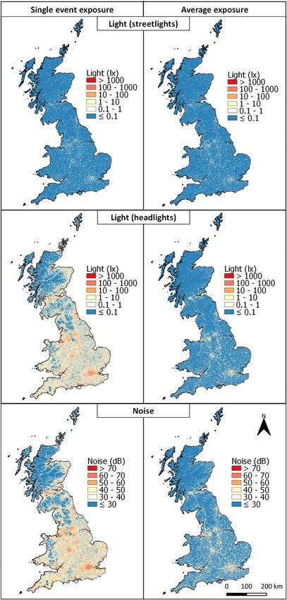
B.B. Phillips, J.M. Bullock, J.L. Osborne et al.                                                                  Science of the Total Environment 773 (2021) 145589

1. Introduction                                                                   whether it consists of energy waves (e.g. light and noise) or matter
                                                                                  (e.g. metals and air pollutants). Specifically, particle pollution such as
    Roads form vast and pervasive networks across the Earth, with an              metals and air pollutants are largely transported via diffusion, whereas
overall estimated length of 64 million km (van der Ree et al., 2015).             light and noise are energy waves travelling via vibrations. Their patterns
The associated pollution and other negative environmental impacts                 of dispersal over distance therefore differ, and in general, can be de-
spill out even further, forming a ‘road-effect zone’. Understanding the           scribed, respectively, by exponential decay and inverse square decay
extent of these impacts is critical for identifying where environmental           functions (Attenborough, 2014; Karner et al., 2010).
protections (e.g. from further road building), environmental mitigations              Whilst numerous models of road pollution exist, they focus on
(e.g. pollution reduction) and environmental enhancements (e.g. habi-             individual forms of pollution, covering a limited subset of pollutants –
tat creation) will most benefit the health of both people and nature. It           primarily air pollutants (Tsagatakis et al., 2019) and noise (Extrium,
can also provide insights into how the environmental impacts of roads             2020). They are usually limited to a local scale (meters to kilometres
will be affected by future changes in road use (e.g. road growth and in-          rather than hundreds of kilometres) in urban areas, and are often com-
creasing traffic volumes) and associated technologies (e.g. uptake of              plex, requiring extensive data sources, parameter estimates and compu-
ultra-low emission vehicles).                                                     tational power (e.g. see Bendtsen, 1999; Forehead and Huynh, 2018;
    Previous attempts to understand the impacts of roads on the envi-             Khan et al., 2018; Murphy et al., 2020; Pinto et al., 2020; Silveira et al.,
ronment over large regions have generally related road proximity to               2019). Or, otherwise, they model only the largest road types (Extrium,
specific environmental impacts, often using single thresholds for the ex-          2020) and ignore the potential contribution of smaller roads. Here,
tent of the road-effect zone (e.g. 1 km) (Forman, 2000; Ibisch et al.,            using Great Britain as a study area and considering diverse forms of pol-
2016; Psaralexi et al., 2017; Torres et al., 2016). Such approaches have          lution, we determine the spatial distribution of road pollution, with re-
estimated that 20% of land suffers environmental impacts of roads                 spect to distance from roads and types of road. The study aims to: 1.
(though the underlying global road maps are very incomplete for                   Provide a more complete understanding of the road-effect zone by con-
some regions) (Hughes, 2017; Ibisch et al., 2016). Whilst there is a              sidering diverse forms of pollution; and 2. Provide a national-scale as-
strong environmental case for preserving roadless areas (often defined             sessment as a case study for determining the proximity of land to
as areas more than 1 km from any road; Ibisch et al., 2016; Psaralexi             roads and the proportion of land affected by different threshold levels
et al., 2017; Selva et al., 2011), many regions have few such areas re-           of pollution. The findings are important for understanding the extent
maining (e.g. central and western Europe; Psaralexi et al., 2017), and            and degree of roads' influences on the environment, with implications
roads provide important social and economic benefits that motivate fur-            for both human and ecosystem health.
ther road building (Laurance et al., 2014). Indeed, roadless areas will
likely become increasingly scarce, given that the global road network             2. Methods
is predicted to expand by a further 25 million paved road lane-
kilometres (a 65% increase) by 2050 (Dulac, 2013). As a result, there is              We used spatial mapping and analyses in QGIS 3.4.15 (QGIS
a need to go beyond identifying ‘where is’ versus ‘where is not’ affected         Development Team, 2020) to determine the distribution of road pollu-
by roads, and towards understanding how the intensity of environmen-              tion across Great Britain. The process involved the following steps, de-
tal impacts of roads varies across space, in terms of different types of          scribed in detail below and summarised here: (i) categorising roads
impact.                                                                           into four types based on their traffic volumes and mapping the distance
    In reality, the intensity of road impacts shows spatial complexity, de-       of every 1 ha square of land in GB to roads of each type; (ii) creating gen-
creasing with distance from the road and often increasing with traffic             eral models of the spatial distribution of different forms of road pollu-
volume. Furthermore, the environmental impact of roads is the result              tion based on the following parameters: pollution source strength
of diverse forms of pollution, including light, noise, vibration, de-icing        across road types, background pollution level, and pollution dispersion
salt, metals, herbicides, and exhaust emissions (e.g. NOx, CO and                 pattern with distance from the road; (iii) conducting a literature search
particulates), alongside other effects (e.g. habitat fragmentation and            to determine known parameter values for different forms of road pollu-
vehicle-wildlife collisions) (Forman et al., 2003). Of these, noise and           tion (metals (Cd, Cr, Cu, Ni, Pb, and Zn), air pollutants (NO2, PM2.5 and
air pollution have received by far the most attention due to their im-            PM10), light and noise); (iv) modelling spatial distributions for these
pacts on human health, for which they are considered to be the most               forms of road pollution by parameterising the models from (ii) with
prevalent environmental risk factors in Europe (Hänninen et al.,                  values from (i) and (iii); and (v) generalising our findings, given limita-
2014). Roads are a major contributor to both. In fact, the World Health           tions on available data for real forms of road pollution, by modelling
Organization (2011) states that “sleep disturbance and annoyance,                 spatial distributions of theoretical pollution groups that differ in the
mostly related to road traffic noise, comprise the main burden of envi-            outlined parameters, across a range that encompasses those of real
ronmental noise”. However, whilst air pollution is regulated in many              forms of road pollution.
countries, with strict limits on roadside pollution and emissions from in-
dividual vehicles (European Commission, 2021a, 2021b), noise pollu-               2.1. Spatial maps of road proximity
tion is scarcely regulated or enforced. Whilst recommended limits
exist (World Health Organization, 2018), these guidelines are rarely                  To map roads, we used freely available data from OS OpenData
backed up by legislation. For example, in the UK there are noise limits           (Ordnance Survey, 2020): OS Open Roads and OS Boundary-Line. OS
for individual vehicles, but no legal limits for road noise overall (UK           Open Roads is a vector map of all roads in Great Britain, including infor-
Government, 2021). Furthermore, the diverse other forms of road pollu-            mation on road classification. OS Boundary-Line contains vectors of
tion are almost completely ignored by policy.                                     Great Britain and its administrative boundaries. We merged component
    Different forms of road pollution vary in their spatial distributions         layers of OS Open Roads into a single shapefile and removed duplicated
with respect to roads, in particular how they attenuate over distance.            sections of road. We aggregated roads into four types (which we will
Many pollutants are deposited near to roads, for example metals arising           term r) based on road classification (from OS Open Roads) and the avail-
from vehicles and road surfaces are principally found in soils within             ability of associated traffic volumes (from UK Government data;
15 m of roads (Werkenthin et al., 2014). Other pollutants are more far            Department for Transport, 2019) (Table 1). These types were (in order
reaching, with many air pollutants found at elevated levels at distances          of highest to lowest traffic volume) motorways, A-roads, minor roads,
of hundreds of meters from roads (Karner et al., 2010). Whilst disper-            and local access roads.
sion patterns are highly variable among pollutants, in the broadest                   We created a grid of points with 100 m intervals across the extent of
sense the way that a pollutant attenuates over distance depends on                Great Britain, then clipped the grid using a polygonised high-water

                                                                              2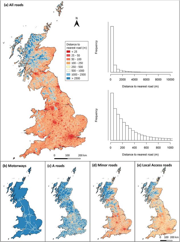
B.B. Phillips, J.M. Bullock, J.L. Osborne et al.                                                                                           Science of the Total Environment 773 (2021) 145589

    Table 1
    The road types r that were used for the spatial mapping and analyses of road pollution. Maps of the proximity to roads of each road type are provided in Fig. 1b–e.

      Road type r               OS Open Roads road class(es)                  OS Open           UK                 Proportion of UK Government traffic volume                  Relative
                                                                              Roads road        Government         total         (vehicles day−1)b                            traffic
                                                                              length (km)       road               road length                                                volume
                                                                                                length (km)a

      Motorways                 Motorways                                        5141           3742               0.0074         81,700                                      1.0000
      (r = 1)
      A-roads                   A-roads                                        49,659           47,450             0.0719         13,800                                      0.1689
      (r = 2)
      Minor roads               B/Minor/Local roads                           341,684           346,405            0.4947         1400                                        0.0171
      (r = 3)
      Local access roads        Local Access/ Restricted Local                294,196           Not provided       0.4260         Not available, so assumed 70                0.0009
      (r = 4)                   Access/Secondary Access roads                                                                     (5% of minor roads)
      a
          Department for Transport (2020). Road lengths statistics (RDL). Data for 2019. https://www.gov.uk/government/statistical-data-sets/road-length-statistics-rdl.
      b
          Department for Transport (2019). Road traffic statistics (TRA) statistical data set. Data for 2018. https://www.gov.uk/government/statistical-data-sets/road-traffic-statistics-tra.

polyline shapefile from OS Boundary-Line. We calculated the distance to                              describe throughout. In general though, we used average values across
the centreline of the nearest road for each grid point, then converted                              space and time, whereas traffic volumes differ between urban and
this information to a raster with 100 m resolution, resulting in the value                          rural areas, among geographic regions, and across the time of day and
of each cell representing the distance to the nearest road of the centroid                          week (Department for Transport, 2019), and dispersion of pollutants
of the cell (Fig. 1a). We repeated this process for each of the four road                           is affected by meteorological conditions, which can also result in strong
types, resulting in a 100 m raster of distances to the nearest road for                             asymmetry between opposite sides of a road (Forman et al., 2003). We
each road type (Fig. 1b–e). As the distance to the nearest road used a                              did not incorporate pollution mitigation by vegetation, terrain and other
centreline for each road, we accounted for differences in road widths                               barriers, so our estimates are rather representative of maximum poten-
between road types by assuming that: (i) pollution originates from                                  tial extent. We address the implications of these assumptions in the
the centre of the outermost lanes of a road, (ii) road lanes are 3.65 m                             discussion.
wide (Department for Transport, 2020a) and (iii) the number of lanes
per direction is 3 for motorways, 1.5 (1 to 2) for A-roads, 0.75 (0.5 to                            2.2.1. Pollution source strength
1) for minor roads and 0.625 (0.5 to 0.75) for local access roads. We                                   We assumed that differences in pollution source strengths among
therefore subtracted the following distances from all cells (bounded                                road types were related to traffic volumes. This is because most road
above zero) of the respective road type raster: 9.125 m for motorways                               pollutants arise either directly from vehicles (e.g. noise and exhaust
(Fig. 1b), 4.5625 m for A-roads (Fig. 1c), 1.3688 m for minor roads                                 emissions), or indirectly from roads themselves (e.g. particles from
(Fig. 1d) and 1.1406 m for local access roads (Fig. 1e).                                            wear of road surfaces) and their management (e.g. de-icing salt),
    For context, we estimated the area of land covered by roads by mul-                             whereby roads with greater traffic volume are likely to be larger and re-
tiplying the width of a road lane (3.65 m wide; Department for                                      ceive more intensive management (Forman et al., 2003). However, the
Transport, 2020a) by the estimated number of lanes per road of each                                 strength of the relationship between pollution source strength and traf-
road type (see above), then multiplying by the length of road of each                               fic volume likely varies among pollutants and may have a weak relation-
type (from UK Government data for 2019; Department for Transport,                                   ship (e.g. heat originating from the road surface, light originating from
2020; see Table 1). We also assessed the land cover and elevation of                                street lighting) or possibly no relationship. As such, we calculated rela-
roadless areas (>1 km from roads) using CORINE Land Cover                                           tive pollution source strengths for each road type based on the relative
(Copernicus, 2018) and OS Terrain 50 (Ordnance Survey, 2020).                                       impact of traffic volume on the pollution source strength. We used the
                                                                                                    following equation:
2.2. General modelling approach
                                                                                                    ar ¼ ðt r =t 1 Þx                                                                      ð1Þ
    We built two general models of the spatial distribution of road pol-
                                                                                                    where ar is the pollution source strength for road type r, tr is the average
lution: one for pollution caused by energy waves (such as light and
                                                                                                    daily traffic volume for road type r (from UK Government data for 2018;
noise) and one for pollution consisting of matter (such as metals, partic-
                                                                                                    Department for Transport, 2019; Table 1), t1 is the average daily traffic
ulate matter and NO2). These models were later parameterised from the
                                                                                                    volume for the highest traffic volume road type (motorways) and x is
literature for different types of pollution. The modelling approach was
                                                                                                    a scaling variable defining the relative impact of traffic volume on the
based on differences in (i) pollution source strength a (the pollution
                                                                                                    pollution source strength.
level at a road) across road types r (the four road types described
above, differing in traffic volume), (ii) background pollution level b
                                                                                                    2.2.2. Decay rates
(the pollution level in the absence of roads), and (iii) dispersion pat-
                                                                                                        We modelled the attenuation of pollution strength from a point
terns (the function by which pollution disperses from a road, consisting
                                                                                                    source over an uninterrupted linear distance from a road using two dif-
of decay type – inverse square or exponential – and, in the latter case,
                                                                                                    ferent decay functions, which are well established for different forms of
decay rate λ). We modelled levels of pollution exclusively attributable
                                                                                                    pollution. For simplicity, these equations represent the decay from a
to roads by subtracting the background pollution level b from the pollu-
                                                                                                    point source, representing the straight-line distance to the nearest
tion source strength a, which meant that modelled road pollution levels
                                                                                                    road. 1. Inverse square decay, to represent pollution types that consist
attenuated to zero, rather than to the background level. In reality, there
                                                                                                    of energy waves (e.g. light and noise; Attenborough, 2014):
are many other sources of pollutants, which combine to result in overall
pollution levels; but in this case, pollution arising specifically from roads                                            −2
was of principal interest.                                                                          pe ¼ ða−bÞd                                                                            ð2Þ
    Given the large number of complex variables involved in modelling
just a single pollutant (e.g. see Khan et al., 2018; Pinto et al., 2020), it                        where p is the pollution level, a is the pollution source strength, b is the
was necessary to make assumptions and simplifications, which we                                      background pollution level, and d is the distance to the nearest road. 2.

                                                                                                3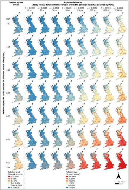
B.B. Phillips, J.M. Bullock, J.L. Osborne et al.                                                                                            Science of the Total Environment 773 (2021) 145589

Fig. 1. Distances to the nearest road from the centre of each 1 ha (0.01 km2) area across Great Britain for (a) all roads, and associated frequency histogram (on two different scales for clarity
of presentation), and (b–e) the four component road types that were used as input parameters for spatial models and analyses of road pollution.

Exponential decay to represent pollution types that consist of matter                               2.2.3. Spatial modelling
(e.g. particulates; Karner et al., 2010):                                                               Using Eqs. (2) and (3), we modelled the pollution level in each
                                                                                                    100 m grid cell attributable to the nearest road of each road type as:
pm ¼ ða−bÞe−λd                                                                           ð3Þ
                                                                                                                           −2
where λ is the decay rate.                                                                          per ðdr Þ ¼ ðar −bÞdr                                                                    ð4Þ

                                                                                                4
B.B. Phillips, J.M. Bullock, J.L. Osborne et al.                                                                     Science of the Total Environment 773 (2021) 145589

for pollution types that consist of energy waves, and                                2.4. Assumptions for missing parameter values

                                                                                         Whilst the literature search provided sufficient parameter values for
pmr ðdr Þ ¼ ðar −bÞe−λdr                                                  ð5Þ
                                                                                     decay rates λ, information on source pollution strengths a and relation-
                                                                                     ships with traffic volume x were mostly lacking. We therefore sought
for pollution types that consist of matter, where ar is the pollution                additional data and were required to make several assumptions
source strength for road type r, and dr is the distance to the nearest road          (Table B). These are described below, with the final parameter values
of road type r (from Fig. 1). We calculated the total pollution level in             for each form of pollution presented in Table 2.
each grid cell by adding together the pollution level attributable to each
of the four road types, resulting in the final equations:                             2.4.1. Metals and air pollutants
                                                                                         For pollution source strengths, we used UK government data for air
            4                                                                        pollutants (NO2, PM2.5, PM10) from 2019 (Table 2; Defra, 2020), which
petotal ¼ ∑ per ðdr Þ                                                     ð6Þ        were similar to the levels measured in the USA by DeWinter et al.
           r¼1
                                                                                     (2018). For both air pollutants and metals, we assumed that median
                                                                                     source strengths from the empirical data were representative of A-
for pollution types that consist of energy waves, and                                roads (r = 2). Source strengths for other road types were proportional
                                                                                     to their traffic volume scaled with x = 0.75 in Eq. (1), rather than x =
             4                                                                       1 (whereby a 10 times increase in traffic volume results in a 10 times in-
pmtotal ¼ ∑ pmr ðdr Þ                                                     ð7Þ        crease in pollution source strength when x = 1, and in a 5.62 times in-
           r¼1
                                                                                     crease in pollution source strength when x = 0.75), because we
                                                                                     assumed that vehicles on smaller, lower traffic roads brake and acceler-
for pollution types that consist of matter. This assumes that pollution              ate more frequently, resulting in a proportionally greater amount of
from multiple roads of different types is additive, but ignores additional           metals and air pollutants (Pandian et al., 2009). However, for PM2.5
nearby roads of the same type (e.g. in urban areas where numerous mi-                we used Eq. (1) with x = 0.5 (whereby a ten-fold increase in traffic vol-
nor roads are located within a small area, resulting in overlapping, addi-           ume results in a 3.16 times increase in pollution source strength) to re-
tive accumulation of pollution, such as around junctions). It also                   flect a weaker relationship between traffic volume and source pollution
assumes that the pollution level in a cell is not affected directly by the           strength (DeWinter et al., 2018). Reviews of NO2 dispersion provided
pollution level in neighbouring cells.                                               dramatically different decay rates of λ = 0.0064 (Karner et al., 2010)
                                                                                     and λ = 0.0004 (Liu et al., 2019), which is equivalent to a ten-fold dif-
2.3. Literature search for parameter values                                          ference in extent. This is apparently because Liu et al. (2019) did not ac-
                                                                                     count for background pollution levels. We therefore used the more
    We conducted a literature search to find parameter values for differ-             conservative and relevant estimates from Karner et al. (2010). We
ent forms of road pollution. We searched Web of Science Core Collection              note that air pollution dispersion patterns from the literature are pri-
databases (in English language only) for scientific publications pub-                 marily based on downwind measurements (Karner et al., 2010; Liu
lished up to January 2020. We limited the search to reviews and                      et al., 2019), whereas in reality dispersion patterns are asymmetrical
meta-analyses due to an abundance of literature on the topic, and only               due to wind direction, and predominant in one direction due to prevail-
to those which focused on Europe and/or North America to ensure rel-                 ing winds. For simplicity, we use downwind dispersion patterns in all
evance to Great Britain (in terms of road and vehicle technologies and               directions, which indicates the maximum potential extent of air
usage). We used a ‘road pollution’ search string and combined it with                pollutants.
a ‘dispersion’ search string (Table A). We assessed the relevance of
each search result using the title and abstract (or full text where neces-           2.4.2. Light and noise
sary). Of 471 search results, we identified five relevant studies, which                   Light and noise arising from vehicles consist of both an intensity and a
provided information on the spatial distributions, with respect to                   frequency component, which are both likely to be relevant in triggering
roads, of metals in soils (Werkenthin et al., 2014), air pollutants                  ecological responses. We therefore considered both single event
(DeWinter et al., 2018; Karner et al., 2010; Liu et al., 2019), and light pol-       exposure level (i.e. when a vehicle passed), and average exposure level,
lution from streetlights and from vehicle headlights (Gaston and Holt,               which accounts for differences in traffic volume between road types.
2018). In each case, we used the full text to extract the following infor-               Noise is commonly expressed in units of decibels – a logarithmic
mation (where available) for each form of pollution: source strength a,              scale which is used as a more representative measure of the perception
background level b, decay rate λ (or otherwise pollution level at multi-             of changes in noise intensity by biological organisms. We therefore con-
ple distances), and the relationship between pollution level and traffic              verted to and from source and estimated noise levels in terms of the log
volume. We used WebPlotDigitizer 4.2 (Rohatgi, 2015) to extract infor-               scale of decibels using the standard equation dB = 10 log p, where p is
mation from figures where necessary. Karner et al. (2010) provided re-                the sound power ratio, which is the unit that decays over distance fol-
gressions of pollution level over distance, rather than explicit decay               lowing the inverse square law. We assumed that noise exposure source
rates, so we extracted the distance at which the pollution level had                 strength was 85 dB for all road types (Bendtsen, 1999). Whilst heavy ve-
decayed by 90% from the source strength towards the background                       hicles and vehicles travelling at greater speeds produce more noise
level, then used this to calculate an exponential decay rate. We used a              (Bendtsen, 1999), which are likely to be more common on motorways
level of 90% because we assumed that the underlying pollution mea-                   and A-roads, such noise levels probably often occur across all road
surement data has low power when it comes to detecting pollution                     types because component roads are highly heterogeneous, and speed
levels that have more closely approached the background level (the                   limits are similar across road types (70 mph (113 km h−1) for motor-
tail of the exponential decay curve). Similarly, Werkenthin et al.                   ways, and most frequently 60 mph (97 km h−1) for other road types
(2014) only provided pollution levels for three distance categories                  because we didn't distinguish urban from rural roads). For average
(0–5, 5–10 and 10–25 m from roads), so we calculated a decay rate                    noise exposure level, we estimated source strengths for each road
based on changes in the median pollution level across distance catego-               type using Eq. (1) with a1 = 85 dB and x = 1. These assumptions result
ries – resulting in either λ = 0.2303 or λ = 0.0921, reflecting 90% decay             in average noise source strengths for each road type that are similar to
of pollution source strength towards the background level by 10 and                  those used in previous national-scale modelling of noise across Great
25 m, respectively.                                                                  Britain (Jackson et al., 2008).

                                                                                 5
B.B. Phillips, J.M. Bullock, J.L. Osborne et al.                                                                                           Science of the Total Environment 773 (2021) 145589

    Table 2
    Summary of the model parameter values, including those informed by the literature search (λ, a and b), and those that were otherwise estimated (primarily x; see Methods). These
    parameters were used to produce Figs. 2–3. Full details, including assumptions and limitations of these synthesised parameters, are described in Table B.

      Form of road                      Units      Decay type       Source pollution level ~ traffic     Decay      Pollution source   Background             Data sources
      pollution                                                     scaling factor (x)                  rate (λ)   strength (a)       pollution level (b)

      Light pollution
      Streetlights
        Single event exposure           lx         Inverse square   n/a                                 n/a        4800                0                     Gaston and Holt (2018)
        Average exposure                                            (1,1,0,0 for r = 1,2,3,4)           n/a        4800                0
        Vehicle headlights
        Single event exposure                                       0                                   n/a        9200                0
        Average exposure                                            1                                   n/a        9200                0

      Noise pollution
      Single event exposure             dB         Inverse square   0                                   n/a          85                0                     Attenborough (2014)
      Average exposure                                              1                                   n/a          85                0

      Metal pollution
      Cadmium (Cd)                      ppm        Exponential      0.75                                0.0921        0.73             0.21                  Werkenthin et al. (2014)
      Chromium (Cr)                                                 0.75                                0.2303       28.0             25.7
      Copper (Cu)                                                   0.75                                0.2303       47.9             13.6
      Nickel (Ni)                                                   0.75                                0.2303       24.5             20.2
      Lead (Pb)                                                     0.75                                0.0921      106.0             23.5
      Zinc (Zn)                                                     0.75                                0.2303      179.5             52.9

      Air pollutants
      NO2                               ppb        Exponential      0.75                                0.0064       31                7                     Defra (2020);
      PM2.5                                                         0.5                                 0.0023       10.08             9.87                  DeWinter et al. (2018);
      PM10                                                          0.75                                0.0200       18               15                     Karner et al. (2010)

    Vehicle headlights produce a concentrated horizontal beam that at-                                which is known to have ecological impacts (Gaston et al., 2013;
tenuates at a lower rate than described by an inverse square decay, but                               Sanders et al., 2020). For noise 0.001% is equivalent to 30 dB – above
this is generally directed largely parallel rather than perpendicular to a                            which effects on human sleep are observed (Basner and McGuire,
road so we also assumed that decay of this light perpendicular to the                                 2018). Levels above 0.1% for matter, and above 0.001% for energy
road follows an inverse square relationship. For light arising from street-                           waves, are therefore described as elevated. This cut-off was necessary
lights, we assumed that streetlights are always turned on at night-time                               because exponential and inverse square decay functions have long
(so the single event exposure level, as used for noise and light from ve-                             tails that approach, but never reach, zero. For each pollutant, we calcu-
hicle headlights, is equivalent to the average exposure level), and that                              lated the proportion of raster cells above threshold pollution levels of in-
they are found on all motorways and A-roads, but not on minor roads                                   terest, then converted this to an estimate of land area (km2).
or local roads (Table 2). In reality, streetlights are often found along
minor roads in urban areas, but these were not distinguished from                                     2.5.2. Theoretical road pollution groups
rural roads in our road type groupings.                                                                   Given limitations on available data for different forms of road pollu-
                                                                                                      tion, we modelled the spatial dispersion of theoretical pollution groups
2.5. Spatial modelling                                                                                that varied in their pollution source strengths and dispersion patterns,
                                                                                                      across a range that encompasses those of real forms of road pollution.
2.5.1. Real forms of road pollution                                                                       We considered nine values of x (1.5, 1.25, 1, 0.75, 0.5 0.25, 0.1, 0.05,
    We modelled, in absolute terms, the spatial distributions of metals in                            and 0) that covered the full realistic range of relationships between traf-
soils (Cd, Cr, Cu, Ni, Pb, and Zn), of air pollutants (NO2, and particulate                           fic volume and pollution source strength, from disproportionately large
matter PM2.5 and PM10) (particles), and of light and noise (energy                                    effects (x > 1), to simple additive effects (x = 1), to increasingly
waves) arising from roads. Modelling used Eqs. (1)–(7), combined                                      diminishing effects (x < 1), of increasing traffic volume (Table C). As
with parameter values gathered from the literature search, and supple-                                the modelled pollution level was relative, rather than absolute, the
mented with the estimates and assumptions described above to provide                                  background pollution level b was not required. We considered values
missing values (Table 2).                                                                             for decay rates λ that resulted in the pollution level decreasing by 90%
    We describe the spatial distribution of pollution consisting of matter                            of its source strength at distances of 10, 25, 50, 100, 250, 500, 1000,
using thresholds of 50%, 25%, 10%, 1%, and 0.1% of the source strength                                and 2500 m from the source, a total of eight different decay rates
found along the busiest road type (motorways). Whilst 0.1% appears                                    (Table C). We considered all combinations of pollution source strengths
to be small, it is equivalent to elevated levels of 0.002 ppm Cd,                                     a (values of x in Eq. (1)), and decay rates λ for models of pollution types
0.01 ppm Cr, 0.13 ppm Cu, 0.02 ppm Ni, 0.31 ppm Pb, 0.48 ppm Zn,                                      that consist of matter – a total of 81 pollution groups (Fig. A; Table C).
0.09 ppb NO2, 0.0005 ppb PM2.5, and 0.01 ppb PM10 (Fig. 2). These
metal concentrations are similar to the maximum guidelines for drink-                                 3. Results
ing water (World Health Organization, 2017) and, for example, such
levels of lead have been found to have effects on animal physiology                                   3.1. Distance to nearest road
(Boskabady et al., 2018). Real measurements of pollution levels will
generally be much greater because our models do not include back-                                         Using 100 m resolution maps to calculate the distance of each 100 m
ground levels or pollution from non-road sources. For light and noise                                 centroid to the nearest road, shows that 25% of land is less than 79 m
(energy waves), we use thresholds of 10%, 1%, 0.1%, 0.01%, and 0.001%                                 from a road, 50% less than 216 m and 75% less than 527 m (Fig. 1). In
of the source strength (Fig. 3) because a logarithmic scale is more repre-                            most cases, the nearest road is a minor or local access road, as these con-
sentative of the perceived changes in these forms of pollution by organ-                              stitute 49% and 43%, respectively, of total road length, compared to the
isms. For light 0.001% of the source strength is equivalent to elevated                               8% of total road length that comprises more major roads (motorways
levels of 0.1 lx – comparable to full moonlight under a clear sky,                                    and A-roads; Table 1). Roadless areas (>1 km from roads) are scarce,

                                                                                                6
B.B. Phillips, J.M. Bullock, J.L. Osborne et al. Science of the Total Environment 773 (2021) 145589
Fig. 2. The modelled spatial distributions of metals and air pollutants arising from roads across Great Britain. Values are pollution levels exclusively attributable to roads, i.e. additional
pollution produced by roads beyond the background level, rather than the absolute pollution level (incorporating all sources). Maps were produced using Eqs. (1)–(7) and the
parameter values in Table 2.
covering only 11.8% of land, and confined almost exclusively to the up- land covers: 47% peat bogs, 23% moors and heathland, 14% natural
lands (Fig. 1). Specifically, these areas have a mean elevation of 391 m grasslands, and 8% sparsely vegetated areas. Only 3.6% of land is more
(median = 386 m, SD = 218 m), and are composed of the following than 2.5 km from roads (Fig. 1). For comparison, based on a total length
7B.B. Phillips, J.M. Bullock, J.L. Osborne et al. Science of the Total Environment 773 (2021) 145589
Fig. 3. The modelled spatial distributions of light and noise arising from roads across Great Britain. Values are pollution levels exclusively attributable to roads, i.e. additional pollution
produced by roads beyond the background level, rather than the absolute pollution level (incorporating all sources). Single event exposure level represents the typical level
experienced when a vehicle passes on the nearest road, whereas average exposure level accounts for differences in traffic volume between road types. Maps were produced using
Eqs. (1)–(7) and the parameter values in Table 2.
8B.B. Phillips, J.M. Bullock, J.L. Osborne et al. Science of the Total Environment 773 (2021) 145589
Table 3 Table 3 (continued)
Estimated area of land in Great Britain affected by different forms of road pollution (from
Figs. 2–3). Form of road pollution Pollution Estimated area of land in
level Great Britain affected
Form of road pollution Pollution Estimated area of land in
Area of land % of
level Great Britain affected
(km2) land
Area of land % of
PM10 in air >5.00 ppb 1837 0.88
(km2) land
>2.50 ppb 352 0.17
Light (streetlights) – single event >1000 lx 374 0.18 >1.25 ppb 4737 2.26
exposure level >100 lx 1104 0.53 >0.125 ppb 41,638 19.89
>10 lx 2492 1.19 >0.0125 ppb 83,493 39.89
>1 lx 6667 3.18
>0.1 lx 19,109 9.13
Light (streetlights) – average exposure >1000 lx 374 0.18
level >100 lx 1104 0.53 of road of 690,680 km across Great Britain (including the 294,196 km of
>10 lx 2492 1.19 local access roads, which are generally not considered in national esti-
>1 lx 6667 3.18
mates of road length; Table 1), we estimate that roads cover 1934 km2
>0.1 lx 19,109 9.13
Light (headlights) – single event >1000 lx 4300 2.05 (0.8% of land), with an average road density of 2.84 km of road/km2 of
exposure level >100 lx 11,044 5.28 land. This estimate includes the paved road surface, but not related
>10 lx 29,567 14.12 hard and soft surfaces either side of, or in between, road lanes (e.g.
>1 lx 71,134 33.98 pavements, laybys, central reservations, and road verges).
>0.1 lx 147,220 70.33
Light (headlights) – average exposure >1000 lx 178 0.09
level >100 lx 1743 0.83 3.2. Spatial distribution of real forms of road pollution
>10 lx 4928 2.35
>1 lx 13,683 6.54 Considering real forms of road pollution for which there were data to
>0.1 lx 35,360 16.89
estimate their patterns of spread from roads, high levels (e.g. >10% of
Noise – single event exposure level >70 dB 5142 2.46
>60 dB 13,316 6.36 source strength) are relatively localised (Figs. 2–3). However, elevated
>50 dB 33,838 16.16 levels occur across an estimated 94% of land in Great Britain, especially
>40 dB 77,124 36.84 for NO2, PM2.5, noise and light (Figs. 2–3). Again, the only land to escape
>30 dB 147,147 70.29 pollution from roads is located almost entirely in the uplands.
Noise – average exposure level >70 dB 458 0.22
>60 dB 3346 1.60
The proportion of land affected by 10% or more of the pollution
>50 dB 8728 4.17 levels found at the source along the busiest roads amounts to 9% for
>40 dB 23,133 11.05 NO2 and 52% for PM2.5. The respective proportion of land affected by
>30 dB 55,834 26.67 1% or more of these pollutants is 51% for NO2, 84% for PM2.5, and by
Cadmium (Cd) in soils >1 ppm 138 0.07
0.1% or more is 77% and 94%. Based on estimated concentrations of
>0.5 ppm 644 0.31
>0.25 ppm 1356 0.65 these pollutants at roadsides, 45% of land is affected by NO2 levels ele-
>0.025 ppm 12,787 6.11 vated by at least 1.25 ppb due to roads, and 88% of land in Great Britain
>0.0025 ppm 30,363 14.50 is affected by PM2.5 levels elevated by at least 0.005 ppb due to roads.
Chromium (Cr) in soils >5.00 ppm 202 0.10 Due to the pervasiveness of roads, and of light and noise arising from ve-
>2.50 ppm 489 0.23
>1.25 ppm 777 0.37
hicles on them, most land is likely to be exposed to some pollution. For
>0.125 ppm 5641 2.69 example, when vehicles pass by on nearby roads, an estimated 70% of
>0.0125 ppm 13,977 6.68 land in Great Britain is exposed to elevated light pollution of at least
Copper (Cu) in soils >60.00 ppm 295 0.14 0.1 lx, and to elevated noise pollution of at least 30 dB (0.001% of the
>30.00 ppm 582 0.28
source strength found along the busiest road type – motorways). Taking
>15.00 ppm 868 0.41
>1.50 ppm 6300 3.01 account of the frequency of light and noise pollution due to intermittent
>0.15 ppm 14,838 7.09 traffic, 16% of land is affected by average light levels from roads of at
Nickel (Ni) in soils >10.00 ppm 180 0.09 least 0.1 lx, and 27% of land is affected by average noise levels from
>5.00 ppm 467 0.22 roads of above 30 dB (Fig. 3). Additional results are provided in Table 3.
>2.50 ppm 756 0.36
>0.25 ppm 5488 2.62
>0.025 ppm 13,778 6.58 3.3. Spatial distribution of theoretical road pollution groups
Lead (Pb) in soils >50.00 ppm 1117 0.53
>25.00 ppm 1833 0.88 Given limitations on available data for the dispersion of different
>12.50 ppm 4524 2.16
pollutants from roads, we generalised our findings by modelling the
>1.25 ppm 21,302 10.18
>0.125 ppm 38,283 18.29 spatial dispersion of theoretical pollution groups with different charac-
Zinc (Zn) in soils >250.00 ppm 245 0.12 teristics. Again, this shows that high levels of road pollution (e.g. >10%
>125.00 ppm 531 0.25 source strength) are generally localised (Figs. 4–5). However, pollution
>62.50 ppm 818 0.39 need only extend 250 m or more from roads, even if highly concentrated
>6.25 ppm 5942 2.84
around high traffic volume roads, for it to affect at least 50% of land in
>0.625 ppm 14,368 6.86
NO2 in air >50.00 ppb 834 0.40 Great Britain at levels above 0.1% of those found alongside the busiest
>25.00 ppb 2762 1.32 roads (Figs. 4–5). Overall, minor roads and local access roads have
>12.50 ppb 13,104 6.26 major potential to cause widespread pollution and environmental im-
>1.25 ppb 94,973 45.37
pacts due to their substantially greater extent than motorways and A-
>0.125 ppb 157,290 75.14
PM2.5 in air >0.2 ppb 16,872 8.06
roads (Table 1). As the dispersal distance of a pollutant increases –
>0.1 ppb 48,375 23.11 from a 90% decay within 10 m to a 90% decay within 250 m – the total
>0.05 ppb 111,298 53.17 land area affected rapidly increases, regardless of whether pollution pri-
>0.005 ppb 183,718 87.76 marily arises from high traffic roads or more evenly across road types
>0.0005 ppb 197,691 94.44
(Figs. 4–5). However, for forms of pollution arising primarily from
high traffic volume roads, pollution is far more localised. Overall,
9B.B. Phillips, J.M. Bullock, J.L. Osborne et al. Science of the Total Environment 773 (2021) 145589
10B.B. Phillips, J.M. Bullock, J.L. Osborne et al. Science of the Total Environment 773 (2021) 145589
Fig. 5. The proportion of land in Great Britain affected by (a) ≥50%, (b) ≥10%, (c) ≥1% and (d) ≥0.1% of the maximum pollution source strength (i.e. that observed along motorways – the
highest traffic volume road type), for each theoretical pollution group – varying in decay type: inverse square or exponential with varying decay rate, λ, and relative impact of traffic
volume on pollution source strength (x), i.e. level of clustering of pollution around high traffic volume roads (see Eqs. (1)–(7) and Table C). These data summarise the patterns in Fig. 4.
theoretical forms of pollution with relatively rapid decay (that decay by protecting roadless areas from further road building for nature conser-
90% within 250 m), and arising primarily from high traffic roads, are vation purposes (Ibisch et al., 2016; Psaralexi et al., 2017; Selva et al.,
present at high levels only over limited extents (i.e. 0.1% of source strength) that makes them even more important. Yet, the limited extent of roadless
might still be environmentally relevant, they can extend across large areas, and the fact that they are located almost exclusively in the up-
areas (i.e. >50% of land) (Fig. 5c–d). For example, pollution that extends lands, shows that protecting them has limited capacity to protect spe-
100 m from roads is still likely to cover more than half of Great Britain, cies and ecosystems that are vulnerable to road pollution, or people's
albeit at low levels (>0.1–1% of source strength), unless arising almost health. Instead, it validates the rationale for our study to look at how
exclusively from high traffic roads (Fig. 5c–d). road impacts vary within road-effect zones.
Our findings have important implications for research and policy.
4. Discussion Namely, we suggest that the extent of roads' influence on the environ-
ment has been somewhat overlooked and underestimated. As with
Using realistic estimates of how pollution levels decay with distance, light pollution and the intensification of agriculture, environmental
our study suggests that, whilst the greatest levels of road pollution are pressures from roads have largely arisen, and rapidly grown, over the
relatively localised, low levels of road pollution are pervasive. Specifi- past 50–100 years, and may now be so pervasive that their effects are
cally, mapping of pollutants for which sufficient data are available difficult to distinguish and disentangle, and so are not fully appreciated.
shows that roads may have a zone of influence (road-effect zone) that Our study justifies a major research effort to evaluate the extent, path-
extends across at least 70% of land in Great Britain, and potentially less ways and impacts of the many poorly studied forms of road pollution.
than 6% of land escapes any impact. This is in strong contrast to the rel- Whilst research is lacking for most forms of pollution and their potential
atively small area of land that roads themselves cover (an estimated environmental impacts, studies of human health suggest that impacts
0.8% of land). Previous studies have emphasised the importance of on people occur across almost the entire range of most air pollutants
Fig. 4. The modelled spatial distribution of road pollution across Great Britain for the theoretical pollution groups that vary in decay type (inverse square or exponential with varying decay
rate, λ) and relative impact of traffic volume on pollution source strength (x), i.e. level of clustering of pollution around high traffic volume roads (see Eqs. (1)–(7) and Table C). Note that
inverse square decay (representing energy wave pollutants, e.g. light) uses a different scale to exponential decay (representing matter pollutants, e.g. gases) because a logarithmic scale is
more representative of the perceived changes in energy wave pollutants by organisms (see Methods).
11B.B. Phillips, J.M. Bullock, J.L. Osborne et al. Science of the Total Environment 773 (2021) 145589
(e.g. up to 100–400 m from roads for particulate matter and 200–500 m 2013). In fact, relatively greater environmental regulation of vehicle
for NO2; Zhou and Levy, 2007), which can have similar respiratory and pollution in the UK likely means that environmental impacts per road
other impacts on birds (Sanderfoot and Holloway, 2017), mammals vehicle are less than in many other regions. Given rapid expansion in
(Llacuna et al., 1996) and insects (Thimmegowda et al., 2020). Recent road networks, and changes in road-use and vehicle technologies over
evidence suggests that road impacts can scale up to population-level ef- the coming decades, there is an urgent need for the environmental in-
fects for birds and mammals (Benítez-López et al., 2010; Cooke et al., fluence of roads to become a more major focus of both research and
2020a, 2020b; Torres et al., 2016), with estimated effects up to distances policy.
of 1 km and 5 km, respectively, so affecting 55.5% and 97.9% of land Supplementary data to this article can be found online at https://doi.
across Europe (Benítez-López et al., 2010; Torres et al., 2016). However, org/10.1016/j.scitotenv.2021.145589.
little is known about if and how impacts on other taxa scale up, or about
how different impacts interact. In summary, the ubiquity of road pollu- CRediT authorship contribution statement
tion should be seriously considered as a potential contributor to global-
and regional-scale environmental issues such as insect declines Benjamin B. Phillips: Conceptualization, Methodology, Investiga-
(Wagner, 2020) and microplastic pollution (Evangeliou et al., 2020). tion, Writing – original draft, Writing – review & editing. James M. Bull-
Looking at effects as they attenuate with distance from roads is more ock: Conceptualization, Methodology, Writing – review & editing,
realistic than assuming a simple cut off with distance, as has previously Supervision. Juliet L. Osborne: Conceptualization, Methodology,
been used (Ibisch et al., 2016; Psaralexi et al., 2017). Whilst a rule of Writing – review & editing, Supervision. Kevin J. Gaston: Conceptuali-
thumb can be assumed whereby further from roads is better, our zation, Methodology, Writing – review & editing, Supervision.
study shows that a mechanistic approach is much more appropriate
because impacts also depend on the type of road, type of pollution Declaration of competing interest
and threshold for environmental impacts. A major advantage of our
study is that we have considered the diverse forms of pollution from The authors declare no competing interests.
roads at large scales. However, we were required by necessity to make
assumptions and simplifications. We can infer that our relatively simple Acknowledgements
models estimate maximum potential extent because we largely ignore
mitigation by vegetation, terrain and other barriers. In reality there is BBP was funded by a NERC GW4+ Doctoral Training Partnership
likely to be much greater spatial and temporal clustering of pollutants (DTP) studentship from the Natural Environment Research Council
and road impacts, for example due to additive effects of multiple nearby (NERC) [NE/L002434/1], with additional funding from the Cornwall
roads of the same type, heterogeneity of traffic volumes between roads Area of Outstanding Natural Beauty unit.
and across time, and local factors such as tall buildings in urban areas
forming street canyons that can trap and thus concentrate air pollutants Data availability statement
(Vardoulakis et al., 2007). However, it should be noted that our study
did not include the influence of streams and rivers in transporting All data supporting the results are provided in the manuscript and
pollutants, or the marine area affected by road pollution, which would appendices, and were gathered or derived from the associated references.
have increased the estimated extent, possibly substantially so if
atmospheric and oceanic currents were accounted for (Evangeliou References
et al., 2020).
Asdrubali, F., D’Alessandro, F., 2018. Innovative approaches for noise management in
Whilst decay rates are available for many pollutants, our study high- smart cities: a review. Curr. Pollut. Reports 4, 143–153. https://doi.org/10.1007/
lights a lack of data on how source pollution strengths vary across road s40726-018-0090-z.
types, or of the environmental impacts of lower levels of road pollution. Attenborough, K., 2014. Sound propagation in the atmosphere. Springer Handbook of
Acoustics https://doi.org/10.1007/978-1-4939-0755-7.
In this case, we estimated a number of parameter values for road pollut-
Basner, M., McGuire, S., 2018. WHO environmental noise guidelines for the european re-
ants (Table 2), then looked across the full range of values (Fig. 4) to gion: a systematic review on environmental noise and effects on sleep. Int. J. Environ.
show how changes in these values would affect the spatial distributions Res. Public Health 15, 519. https://doi.org/10.3390/ijerph15030519.
of these forms of pollution. However, future research should aim to fill Bendtsen, H., 1999. The Nordic prediction method for road traffic noise. Sci. Total Environ.
235, 331–338. https://doi.org/10.1016/S0048-9697(99)00216-8.
these data gaps. Most studies have unsurprisingly focused on the larg-
Benítez-López, A., Alkemade, R., Verweij, P.A., 2010. The impacts of roads and other infra-
est, busiest roads, and on the high levels of pollution found in their im- structure on mammal and bird populations: a meta-analysis. Biol. Conserv. 143,
mediate or near vicinity. However, to comprehend the scale of roads 1307–1316. https://doi.org/10.1016/j.biocon.2010.02.009.
influence on the environment, it is essential to understand the impacts Boskabady, M., Marefati, N., Farkhondeh, T., Shakeri, F., Farshbaf, A., Boskabady, M.H.,
2018. The effect of environmental lead exposure on human health and the contribu-
of pervasive, low levels of pollution. Improvements in sensing technol- tion of inflammatory mechanisms, a review. Environ. Int. 120, 404–420. https://doi.
ogies (e.g. Asdrubali and D'Alessandro, 2018) will increasingly make org/10.1016/j.envint.2018.08.013.
more widespread monitoring of road pollution possible. Cooke, S.C., Balmford, A., Donald, P.F., Newson, S.E., Johnston, A., 2020a. Roads as a con-
Whilst we used Great Britain as a study area, the findings likely apply tributor to landscape-scale variation in bird communities. Nat. Commun. 11, 1–10.
https://doi.org/10.1038/s41467-020-16899-x.
to other densely populated regions at present, and to many additional Cooke, S.C., Balmford, A., Newson, S.E., Donald, P.F., 2020b. Variation in abundances of
regions in the future due to the predicted rapid expansion of the global common bird species associated with roads. J. Appl. Ecol. 1–12. https://doi.org/
road network. Great Britain has road densities towards the upper limit 10.1111/1365-2664.13614.
of those found worldwide – an estimated 2.84 km of road/km2 of land. Copernicus, 2018. CORINE land cover - CLC 2018 [WWW Document]. URL. https://land.
copernicus.eu/pan-european/corine-land-cover.
Whilst we found that distances to roads were somewhat greater than Defra, 2020. ENV02 - air quality statistics [WWW Document]. URL. https://www.gov.uk/
averages reported for the USA (Riitters and Wickham, 2003), for government/statistical-data-sets/env02-air-quality-statistics.
Europe as a whole (Psaralexi et al., 2017; Torres et al., 2016), and world- Department for Transport, 2019. Road traffic statistics (TRA) statistical data set [WWW
Document]. URL. https://www.gov.uk/government/statistical-data-sets/road-traffic-
wide (Ibisch et al., 2016), differences partly reflect the more complete
statistics-tra.
underlying road maps used in our work compared to in previous studies Department for Transport, 2020. Road lengths statistics (RDL) [WWW Document]. URL.
(Hughes, 2017), which included local access roads and other low traffic https://www.gov.uk/government/statistical-data-sets/road-length-statistics-rdl.
roads. In reality, many regions of Europe and North America likely have Department for Transport, 2020a. Design Manual for Roads and Bridges (DMRB).
similarly high densities of roads (Ibisch et al., 2016; Psaralexi et al., DeWinter, J.L., Brown, S.G., Seagram, A.F., Landsberg, K., Eisinger, D.S., 2018. A national-
scale review of air pollutant concentrations measured in the U.S. near-road monitor-
2017) and such densities will increasingly become the norm given a ing network during 2014 and 2015. Atmos. Environ. 183, 94–105. https://doi.org/
forecast 60% growth in the global road network by 2050 (Dulac, 10.1016/j.atmosenv.2018.04.003.
12B.B. Phillips, J.M. Bullock, J.L. Osborne et al. Science of the Total Environment 773 (2021) 145589
Dulac, J., 2013. Global land transport infrastructure requirements: estimating road and Ordnance Survey, 2020. OS OpenData [WWW Document]. URL. https://www.
railway infrastructure capacity and costs to 2050 [WWW Document]. URL. https:// ordnancesurvey.co.uk/opendatadownload/products.html.
webstore.iea.org/global-land-transport-infrastructure-requirements. Pandian, S., Gokhale, S., Ghoshal, A.K., 2009. Evaluating effects of traffic and vehicle char-
European Commission, 2021a. Air quality standards [WWW Document]. URL. https://ec. acteristics on vehicular emissions near traffic intersections. Transp. Res. Part D
europa.eu/environment/air/quality/standards.htm. Transp. Environ. 14, 180–196. https://doi.org/10.1016/j.trd.2008.12.001.
European Commission, 2021b. Air pollution from the main sources - air emissions from Pinto, J.A., Kumar, P., Alonso, M.F., Andreão, W.L., Pedruzzi, R., dos Santos, F.S., Moreira,
road vehicles [WWW Document]. URL. https://ec.europa.eu/environment/air/ D.M., Albuquerque, T.T. de A., 2020. Traffic data in air quality modeling: a review of
sources/road.htm. key variables, improvements in results, open problems and challenges in current re-
Evangeliou, N., Grythe, H., Klimont, Z., Heyes, C., Eckhardt, S., Lopez-Aparicio, S., Stohl, A., search. Atmos. Pollut. Res. 11, 454–468. https://doi.org/10.1016/j.apr.2019.11.018.
2020. Atmospheric transport is a major pathway of microplastics to remote regions. Psaralexi, M.K., Votsi, N.E.P., Selva, N., Mazaris, A.D., Pantis, J.D., 2017. Importance of road-
Nat. Commun. 11, 3381. https://doi.org/10.1038/s41467-020-17201-9. less areas for the European conservation network. Front. Ecol. Evol. 5, 1–8. https://doi.
Extrium, 2020. Extrium noise and air quality viewer [WWW Document]. URL. http:// org/10.3389/fevo.2017.00002.
www.extrium.co.uk/noiseviewer.html. QGIS Development Team, 2020. QGIS Geographic Information System.
Forehead, H., Huynh, N., 2018. Review of modelling air pollution from traffic at street- van der Ree, R., Smith, D.J., Grilo, C., 2015. Handbook of Road Ecology. Wiley Blackwell,
level - the state of the science. Environ. Pollut. 241, 775–786. https://doi.org/ Oxford https://doi.org/10.1002/9781118568170.
10.1016/j.envpol.2018.06.019. Riitters, K.H., Wickham, J.D., 2003. How far to the nearest road? Front. Ecol. Environ. 1,
Forman, R.T.T., 2000. Estimate of the area affected ecologically by the road system in the 125–129. https://doi.org/10.1890/1540-9295(2003)001[0125:HFTTNR]2.0.CO;2.
United States. Conserv. Biol. 14, 31–35. Rohatgi, A., 2015. WebPlotDigitizer [WWW Document]. URL. https://automeris.io/
Forman, R.T.T., Sperling, D., Bissonette, J.A., Clevenger, A.P., Cutshall, C.D., Dale, V.H., WebPlotDigitizer.
Fahrig, L., France, R.L., Goldman, C.R., Heanue, K., Jones, J., Swanson, F., Turrentine, Sanderfoot, O.V., Holloway, T., 2017. Air pollution impacts on avian species via inhalation
T., Winter, T.C., 2003. Road Ecology. Island Press. exposure and associated outcomes. Environ. Res. Lett. 12. https://doi.org/10.1088/
Gaston, K.J., Holt, L.A., 2018. Nature, extent and ecological implications of night-time light 1748-9326/aa8051.
from road vehicles. J. Appl. Ecol. 55, 2296–2307. https://doi.org/10.1111/1365- Sanders, D., Rago, E., Kehoe, R., Patterson, C., Gaston, K., 2020. A meta-analysis of biological
2664.13157. impacts of artificial light at night. Nat. Ecol. Evol. https://doi.org/10.1038/s41559-
Gaston, K.J., Bennie, J., Davies, T.W., Hopkins, J., 2013. The ecological impacts of nighttime 020-01322-x.
light pollution: a mechanistic appraisal. Biol. Rev. 88, 912–927. https://doi.org/ Selva, N., Kreft, S., Kati, V., Schluck, M., Jonsson, B.G., Mihok, B., Okarma, H., Ibisch, P.L.,
10.1111/brv.12036. 2011. Roadless and low-traffic areas as conservation targets in Europe. Environ.
Hänninen, O., Knol, A.B., Jantunen, M., Lim, T.A., Conrad, A., Rappolder, M., Carrer, P., Manag. 48, 865–877. https://doi.org/10.1007/s00267-011-9751-z.
Fanetti, A.C., Kim, R., Buekers, J., Torfs, R., Iavarone, I., Classen, T., Hornberg, C., Silveira, C., Ferreira, J., Miranda, A.I., 2019. The challenges of air quality modelling when
Mekel, O.C.L., 2014. Environmental burden of disease in Europe: assessing nine risk crossing multiple spatial scales. Air Qual. Atmos. Health 12, 1003–1017. https://doi.
factors in six countries. Environ. Health Perspect. 122, 439–446. https://doi.org/ org/10.1007/s11869-019-00733-5.
10.1289/ehp.1206154. Thimmegowda, G.G., Mullen, S., Sottilare, K., Sharma, A., Mohanta, S.S., Brockmann, A.,
Hughes, A.C., 2017. Global roadless areas: hidden roads. Science 355, 1381. https://doi. Dhandapany, P.S., Olsson, S.B., 2020. A field-based quantitative analysis of sublethal
org/10.1126/science.aam6995. effects of air pollution on pollinators. Proc. Natl. Acad. Sci. 117, 202009074. https://
Ibisch, P.L., Hoffmann, M.T., Kreft, S., Pe, G., Kati, V., Biber-freudenberger, L., Dellasala, D.A., doi.org/10.1073/pnas.2009074117.
Vale, M.M., Hobson, P.R., Selva, N., 2016. A global map of roadless areas and their con- Torres, A., Jaeger, J.A.G., Alonso, J.C., 2016. Assessing large-scale wildlife responses to
servation status. Science 354, 1423–1427. https://doi.org/10.1126/science.aaf7166. human infrastructure development. Proc. Natl. Acad. Sci. U. S. A. 113, 8472–8477.
Jackson, S., Fuller, D., Dunsford, H., Mowbray, R., Hext, S., MacFarlane, R., Haggett, C., 2008. https://doi.org/10.1073/pnas.1522488113.
Tranquillity mapping: developing a robust methodology for planning support. Report Tsagatakis, I., Ruddy, M., Richardson, J., Otto, A., Pearson, B., Passant, N., 2019. National At-
to the Campaign to Protect Rural England, Centre for Environmental & Spatial Analy- mospheric Emissions Inventory - UK emission interactive map [WWW Document].
sis. Northumbria University, Bluespace Environments and the University of Newcas- URL. https://naei.beis.gov.uk/emissionsapp/.
tle Upon on Tyne. UK Government, 2021. Noise from roads, trains or planes [WWW Document]. URL.
Karner, A.A., Eisinger, D.S., Niemeier, D.A., 2010. Near-roadway air quality: synthesizing https://www.gov.uk/noise-pollution-road-train-plane/noise-from-roads.
the findings from real-world data. Environ. Sci. Technol. 44, 5334–5344. https://doi. Vardoulakis, S., Valiantis, M., Milner, J., ApSimon, H., 2007. Operational air pollution
org/10.1021/es100008x. modelling in the UK-street canyon applications and challenges. Atmos. Environ. 41,
Khan, J., Ketzel, M., Kakosimos, K., Sørensen, M., Jensen, S.S., 2018. Road traffic air and 4622–4637. https://doi.org/10.1016/j.atmosenv.2007.03.039.
noise pollution exposure assessment – a review of tools and techniques. Sci. Total En- Wagner, D.L., 2020. Insect declines in the anthropocene. Annu. Rev. Entomol. 65,
viron. 634, 661–676. https://doi.org/10.1016/j.scitotenv.2018.03.374. 457–480. https://doi.org/10.1146/annurev-ento-011019-025151.
Laurance, W.F., Clements, G.R., Sloan, S., O’Connell, C.S., Mueller, N.D., Goosem, M., Werkenthin, M., Kluge, B., Wessolek, G., 2014. Metals in European roadside soils and soil
Venter, O., Edwards, D.P., Phalan, B., Balmford, A., Van Der Ree, R., Arrea, I.B., solution - a review. Environ. Pollut. 189, 98–110. https://doi.org/10.1016/j.
2014. A global strategy for road building. Nature 513, 229–232. https://doi.org/ envpol.2014.02.025.
10.1038/nature13717. World Health Organization, 2011. Burden of disease from environmental noise [WWW Doc-
Liu, S.V., Chen, F. Lin, Xue, J., 2019. A meta-analysis of selected near-road air pollutants ument]. URL. https://www.who.int/quantifying_ehimpacts/publications/e94888.pdf.
based on concentration decay rates. Heliyon 5, e02236. https://doi.org/10.1016/j. World Health Organization, 2017. Guidelines for drinking-water quality [WWW Docu-
heliyon.2019.e02236. ment]. URL. https://www.who.int/publications/i/item/9789241549950.
Llacuna, S., Gorriz, A., Riera, M., Nadal, J., 1996. Effects of air pollution on hematological World Health Organization, 2018. Environmental noise guidelines for the European Re-
parameters in passerine birds and small mammals. Arch. Environ. Contam. Toxicol. gion [WWW Document]. URL. https://www.euro.who.int/__data/assets/pdf_file/
31, 148–152. https://doi.org/10.1007/BF00203919. 0008/383921/noise-guidelines-eng.pdf.
Murphy, E., Faulkner, J.P., Douglas, O., 2020. Current state-of-the-art and new directions in Zhou, Y., Levy, J.I., 2007. Factors influencing the spatial extent of mobile source air pollu-
strategic environmental noise mapping. Curr. Pollut. Reports 6, 54–64. https://doi. tion impacts: a meta-analysis. BMC Public Health 7, 1–11. https://doi.org/10.1186/
org/10.1007/s40726-020-00141-9. 1471-2458-7-89.
13You can also read