Future operation of hydropower in Europe under high renewable penetration and climate change - arXiv

Article

 Future operation of hydropower in Europe
 under high renewable penetration and
 climate change
 Ebbe Kyhl Gøtskea , Marta Victoriaa,b

 a
 Department of Mechanical and Production Engineering, Aarhus University
 b
 iCLIMATE Interdisciplinary Centre for Climate Change, Aarhus University
arXiv:2105.07756v1 [physics.ao-ph] 17 May 2021

 SUMMARY
 The balancing provided by hydropower reservoirs is essential in the transition towards
 a decarbonised European energy system, but the resource might be impacted by fu-
 ture climate change. In this work, we first analyse the hydropower operation needed
 to balance a wind and solar dominated European energy system, to signify whether
 and to what extent hydropower is required to operate differently due to the decar-
 bonisation of the energy system. Second, we apply runoff data achieved with 10
 dynamically downscaled climate models with 0.11◦ × 0.11◦ horizontal and daily res-
 olution to project the future reservoir inflow at three CO2 emissions scenarios: low
 (RCP2.6), mid (RCP4.5), and high emissions (RCP8.5). We show that the decar-
 bonised energy system increases the ramp rates and seasonality of the hydropower
 operation. Despite large interannual and intermodel variability, we found a significant
 change in annual inflow due to climate change in 20 out of 22 European countries at
 the mid and high emissions scenarios. The seasonal profile, as well as the frequency
 and duration of droughts and floods, is also projected to be impacted.

 INTRODUCTION
 The power sector is facing a major transformation from using fossil fuel generators
 to renewable and carbon-neutral ones. The European Green Deal proposed by the
 European Commission [1] envisions a climate neutral Europe by 2050. This target
 could be achieved by relying on wind and solar power generation balanced by hy-
 dropower and other dispatchable generators [2]. Hydropower is a substantial part of
 the European electricity generation (accounting for 16% in 2018 [3]) and will remain
 an important energy source in the future. Due to the variable nature of wind and
 solar generation, their increasing penetration in power grids strengthens the need
 for balancing and demands a modifided operation of hydropower plants [4]. Some
 hydropower installations can, however, benefit from wind and solar since they are
 able to contribute to a seasonal dispatch similar to the natural river discharge which
 is favourable for the river ecosystem [5].

 The renewable energy supply is furthermore affected by the changing climate con-
 ditions [6–8]. Most European regions are at the end of the century projected to
 encounter increased wind correlation lengths [9] and higher probability of low wind
 regimes [10]. For solar power, the radiation is projected to decrease in the North-
 ern Europe [9, 11]. Schlot et al. [9] investigated the future European power system
 under climate change impacted series for solar, wind and hydro and found that the
 cost-optimal contribution of solar increases as a result of climate change. This is in
 agreement with the results found by Fonseca et al. [12] for the Southest US. Pre-
 vious studies show that hydropower is particularly sensitive to climate change [9,
 13–17]. Turner et al. [14] apply three general circulation models (GCMs) at a low
 and high emissions scenario in a high-fidelity dam model with a variable hydraulic
 head to project the potential hydropower production for 1,593 globally distributed hy-
 dropower reservoirs at the middle of the century. The authors select hydropower
 reservoirs whose dam and turbine specifications (e.g. dam height, storage capacity,

 1

upstream catchment area, maximum turbine flow rate, etc.) are available. Van Vliet
et al. [15] use a higher number of hydropower plants (24,515) and GCMs (5) but less
information (fixed hydraulic head) for each hydropower plant. Both studies, which
use climate model data of daily temporal and 0.5◦ × 0.5◦ (≈ 50 km × 50 km) horizon-
tal resolution, project a north-south European division in which the Nordic countries
gain an increase in annual hydropower production whereas the Mediterranean and
Balkan countries suffer from a reduction. However, the two studies do not agree on
the outlook for global hydropower. The former projects a change in annual electric-
ity production of ±5% depending on the GCM, whereas the latter projects a robust
(across all GCMs) decrease in the range from 0.4% to 6.1%. Since projections of
hydropower impacts at a global and regional scale are known to vary [6, 7], climate
model uncertainty has been identified as a significant research gap [6]. Moreover,
both aforementioned analyses focus on investigating the impact of climate change
on annual figures and assume that the hydropower operation is independent of the
rest of the power system.

The available energy for electricity production at a hydropower plant is decided by the
local characteristics such as topography, snow formation, temperature, and precipita-
tion which might not be adequately represented in the GCM due to its coarse horizon-
tal resolution. By downscaling the climate model simulation results, using a regional
climate model (RCM), the local and regional characteristics obtain a higher repre-
sentativeness [18]. A comprehensive comparison of the current supply of RCMs for
Europe was conducted by Christensen and Kjellström [18] in which a 5 × 5 GCM-
RCM matrix was analysed for temperature, wind speed, and precipitation. It showed
that the climate model signal was generally more influenced by the choice of GCM
than RCM, but that the RCM has higher influence in mountainous regions due to the
added surface detail. In this work, we concentrate on runoff since the inflow in reser-
voirs is highly correlated to the runoff within the upstream basins of the reservoir [19].
Furthermore, we use an advanced conversion scheme to model inflow from climate
model runoff data in European reservoirs. To our knowledge, a comprehensive anal-
ysis of a large climate model ensemble of runoff with an advanced inflow conversion
scheme has not been conducted before. Two additional novelties of our study are the
use of several RCMs with high resolution and the analysis of climate change impacts
on hydro seasonal profiles, as well as frequency and duration of droughts and floods.

In this work, we investigate the following research question: How is the operation of
reservoir hydropower plants in Europe expected to change in the future? We first
analyse balancing requirements due to high wind and solar penetration in the grids,
and, second, the changed inflow caused by climate change. The former is based
on the 2050 decarbonised cost-optimal European energy system [2], and the lat-
ter on 10 combinations of GCM-RCM runoff climate model data acquired from the
Coordinated Regional Climate Downscaling Experiment (CORDEX) [20]. An em-
phasis is put on the variability caused by the differences between the climate models
(intermodel variability) and within the considered period (interannual variability) to
quantify the robustness and significance of the resulting projection. The time series
that we produce in this project are released under an open license. They include
hourly-resolved time series of inflow for 22 European countries at the beginning of
the century (BOC) from 1991 to 2020 and the end of the century (EOC) from 2071
to 2100, for three CO2 emissions scenarios (RCP2.6 RCP4.5 and RCP8.5), for 10
different climate models, as well as the average of the model ensemble.

METHODS
Sector-coupled European energy model with high wind and solar penetration
The historical operation of hydropower in European countries is compared to the
cost-optimal operation that will be required as the power system decarbonises. For
the latter, hydropower dispatch time series in 2050 obtained with PyPSA-Eur-Sec are
used [2]. The PyPSA-Eur-Sec model optimises the capacity and dispatch of every
generation, storage and transmission technology subject to a global CO2 constraint.
The model assumes perfect competition and foresight as well as long-term market

 2

equilibrium. The system including the electricity and heating sectors is optimised
every 5 years from 2020 to 2050 following a myopic approach, i.e. in every optimi-
sation step, only information regarding that year is available. Technologies installed
in previous time steps remain in the model until they reach the end of their lifetime.
The CO2 constraints in every time step correspond to a carbon budget of 21GtCO2
which enables avoiding human-induced warming above 1.75◦ C with a probability of
>66%, assuming current sectoral distribution for Europe, and equity sharing princi-
ple among regions. The Baseline - Early and Steady pathway in Victoria et al. [2] is
selected.

Modelling hydropower inflow time series under various climate scenarios
Figure 1 presents the methodology applied in this study to obtain country-aggregated
energy inflow time series from climate model data. The time series are obtained
using the location of the hydropower plants [21], the geometry of the upstream basins
[22], and the open-source package Atlite [23]. A detailed description is provided in
Note S1. The methodology to obtain inflow time series was introduced in Liu et al.
[19], where it was used to obtain historical time series in China using reanalysis
weather data.

 Monthly time series Climate model 1096 hydroelectric reservoirs Basin delineations
 22 European countries BOC: 1991 - 2020 22 European countries Level 8 shape files
 2016 - 2019 EOC: 2071 - 2100

 JRC
 ENTSO-E CORDEX HydroSHEDS
 Hydropower
 Historical inflow EUR11 Basins
 database
 Input
 Upstream
 Runoff basin
 determination

 Upstream basin runoff
 aggregation

 Country-level runoff
 aggregation
 Runoff
 aggregation

 Retain factor Inflow conversion
 2016 - 2019

 Energy
 conversion
 1991-2020

 Calibration

 Calibration

 Energy inflow at BOC and EOC
 in 22 European countries
 Results

Figure 1: Scheme of the methodology to obtain hourly resolved inflow time series at the two
 periods, beginning of the century (BOC) from 1991 to 2020 and end of the century (EOC)
 from 2071 to 2100.

Climate model data is acquired from EURO-CORDEX [24] driven by general circu-
lations models from the Coupled Model Intercomparison Project - Phase 5 (CMIP5)
with 0.11◦ ×0.11◦ (≈ 12 km×12 km) horizontal resolution. Every climate model is given
by a combination of a GCM and an RCM. An ensemble consisting of five different
GCMs and two RCMs is applied in this study. Furthermore, each combination is in-

 3

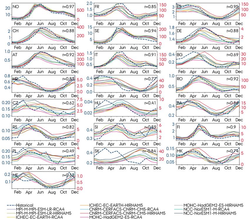
vestigated at three different representative concentration pathways (RCPs), RCP2.6,
RCP4.5, and RCP8.5 [25]. The 5x2x3 matrix of combinations is shown in Table 1.
Although some climate models do not contain data for all RCPs, the three scenarios
are well represented with a total of 6 models assuming RCP2.6, 8 RCP4.5, and 10
RCP8.5, which constitutes an ensemble of 24 climate models. As a preliminary step,
the interannual, inter-RCM, inter-GCM, and climate change-induced variability of the
runoff is evaluated for the RCP8.5 scenario. As a frame of reference, we define the
period from 1991 to 2020 as beginning of the century (BOC) and from 2071 to 2100
as end of the century (EOC). The climate model runoff is indexed with the notation
R̄ijkl in which index i represents the considered period (i = 1 for BOC and i = 2 for
EOC), j the GCM, k the RCM, and l the RCP. The bar indicates the mean annual
value within a period of 30 years.

 GCM
 MPI-ESM-LR[26] EC-EARTH[27] CNRM-CM5[28] HadGEM2-ES[29] NorESM1-M[30]
RCM

RCA4[31] RCP2.6 x x x x
 RCP4.5 x x x x x
 RCP8.5 x x x x x
HIRHAM5[32] RCP2.6 x x
 RCP4.5 x x x
 RCP8.5 x x x x x

 Table 1: Combination of general circulation models (GCMs), regional climate models
 (RCMs), and representative concentration pathways (RCPs) considered in this study.

The climate change effect S is determined by comparing the runoff from EOC with
BOC. E.g. the absolute change in mean daily runoff when assuming RCP8.5 is
calculated as:
 R
 Sjk = R̄2jk3 − R̄1jk3 (1)
The climate change effect on the mean annual inflow is evaluated by calculating the
relative change:
 E Ē2jk3 − Ē1jk3
 Sjk = × 100 (2)
 Ē1jk3
The seasonal inflow profiles obtained with the climate models at the BOC period
(1991-2020), prior to calibration, are compared with observed inflow (1991-2019) for
Norway and Spain in Figure 2 which also shows the corresponding monthly retain
factors, RFc,m . The latter represents the runoff water that does not reach the dam
due to evaporation, groundwater infiltration, etc., and it also includes the model bias
correction. Similar plots for the remaining countries are shown in Figure S10 and
S11. The comparison shows a strong correlation (Pearson correlation r > 0.75)
between the modelled and observed mean monthly inflow for 14 countries. Countries
in the Balkan Peninsula and north of it show moderate correlations (r < 0.75).

RESULTS AND DISCUSSION
Changes in the hydropower operation as wind and solar penetration increases
For the sake of clarity, we focus the discussion on hydropower in Norway and Spain
as countries representative of Northern Europe and Mediterranean climates and
which are projected to experience contrasting impacts of the decarbonisation of the
energy system [2] and of climate change on hydro resources [14, 15]. Figures in
Supplementary material S3 extend the analysis to other countries. Figure 3 presents
the intraday and seasonal profile of the hydroelectricity from historical observations
and a cost-optimised model of the European energy system in 2020 and 2050. The
modelled intraday operation in 2020 is within the historical range in both countries
and captures the morning and afternoon peaks caused by the load curve. The mod-
elled intraday generation in 2050 shows a minimal change in the profile for Norway,

 4

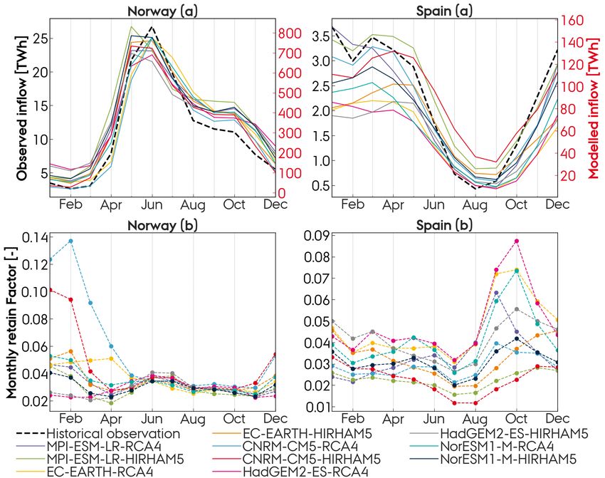
Figure 2: (a) Comparison of modelled, prior to calibration, average monthly inflow at BOC
 period (1991-2020) and observed inflow (1991-2019), and (b) the corresponding retain
 factors estimated according to Eq. 8 for Norway and Spain. In (a) right axis is modelled and
 left axis is observed inflow. Similar plots for other countries are shown in Figures S10 and
 S11.

 Norway (a) 14 Spain (a) 32
 24
 22 7 30
 El. demand [GWh]

 El. demand [GWh]

 20 13 6
Dispatch [GWh]

 Dispatch [GWh]

 28
 18 5
 16 12 4 26
 14 3 24
 12 11 2
 10 22
 1
 0 2 4 6 8 10 12 14 16 18 20 22 10 0 2 4 6 8 10 12 14 16 18 20 22 20
 Norway (b) 8 Spain (b)
 11 23
 18 7
 6 22
 El. demand [TWh]

 El. demand [TWh]

 16
Dispatch [TWh]

 Dispatch [TWh]

 10 5 21
 14
 12 4 20
 9 3
 10 19
 8 2
 8 1 18
 6 0
 Feb Apr Jun Aug Oct Dec7 Feb Apr Jun Aug Oct Dec17
 Modelled (2020) Historical mean (2016-2019)
 Modelled (2050) Historical range (2016-2019)
 Figure 3: Modelled and observed (a) intraday and (b) seasonal operation of hydropower
 plants. The shaded grey area indicates the range of the historical observations. Similar plots
 for other countries are shown in Figure S7.

 whereas Spain shifts from matching the load curve in 2020 to showing a binary op-
 eration. The day-night switch can be explained by the large installation of solar ca-
 pacity in Spain which provides high generation at day but requires balancing at night.

 5

The modelled hydropower does not resemble the historical seasonal dispatch as well
 as the intraday profiles. In 2020, modelled dispatch in both countries show a lower
 magnitude during summer and higher during winter, relative to the historical values.
 In addition, Spain shows a short generation peak in July caused by high electricity de-
 mand. The model assumes perfect foresight (i.e. the weather and inflow are known
 for the entire year) which might cause too ideal operation of hydropower. By 2050,
 the high wind and solar penetration forces the energy system to rely more heavily
 on hydropower during winter. The Spanish hydropower is particularly influenced by
 the solar penetration, showing almost zero dispatch from April to September, and a
 short period during winter with a high level of dispatch.

 Figure 4 illustrates the historical reservoir water inflow and hydropower dispatch,
 which are negatively correlated in Norway. The inflow in Norway has a summer peak
 in June caused by the melting of snow, whereas the dispatch peaks in winter; thus,
 a high share of the hydro resources are saved five months. Conversely, Spain does
 not show such a capability of shifting the seasonal dispatch based on the historically
 strong inflow-dispatch correlation. The inflow in Spain, influenced by rain patterns
 but not by deicing, peaks in winter, while the electricity demand is higher in sum-
 mer. The strong inflow-dispatch correlation in Spain can thus not be explained by
 the electricity demand curve, but instead by the lack of seasonal storage capac-
 ity. This is also illustrated in Figure S8b in which the inflow-dispatch correlation for
 nine countries shows a strong negative correlation with the country-average size of
 the reservoirs (ratio between the energy capacity and power capacity of hydropower
 reservoirs). The increased seasonality in the hydropower operation suggested by
 the model seems, from a historical perspective, feasible in both Norway and Spain
 for different reasons. Norway can meet the seasonally shifted hydropower operation
 due to large reservoirs, whereas Spain is able to comply with increased hydropower
 generation in winter since it is concurrent with the peak inflow. Figure S7 shows the
 intraday and seasonal operation for the remaining countries. For Austria and Roma-
 nia, a similarly increased seasonality is shown in the hydropower operation required
 by the model. However, the two countries are subject to a peak inflow in summer,
 and since the hydropower generation in those countries is correlated with the inflow,
 the modelled operation in 2050 is questionable.

 Norway Spain
 10 r = -0.58
 p = 1.6e-05 2.0 rp==0.82
 6.2e-13
 8
 1.5
 6
[TWh]

 [TWh]

 1.0
 4

 2 0.5

 0 0.0
 Apr Jul Oct Apr Jul Oct Apr Jul Oct Apr Jul Oct Apr Jul Oct Apr Jul Oct Apr Jul Oct Apr Jul Oct
 2016 2017 2018 2019 2016 2017 2018 2019
 Inflow Dispatch
 Figure 4: Observed hydropower reservoir inflow and dispatch from 2016 to 2019 from
 ENTSO-E with r indicating the inflow-dispatch correlation and p the statistical significance.
 Thin lines indicate weekly values and thick monthly averaged. Similar plots for other
 countries are shown in Figure S8.

 The required change in operation may contribute to higher ramp rates which can lead
 to a reduced lifetime of the hydropower plants due to higher mechanical stresses [33].
 See Supplementary Figure S9. This is consistent with previous studies [4] and [34]
 which showed the same effect when only increasing the wind power capacity in a

 6

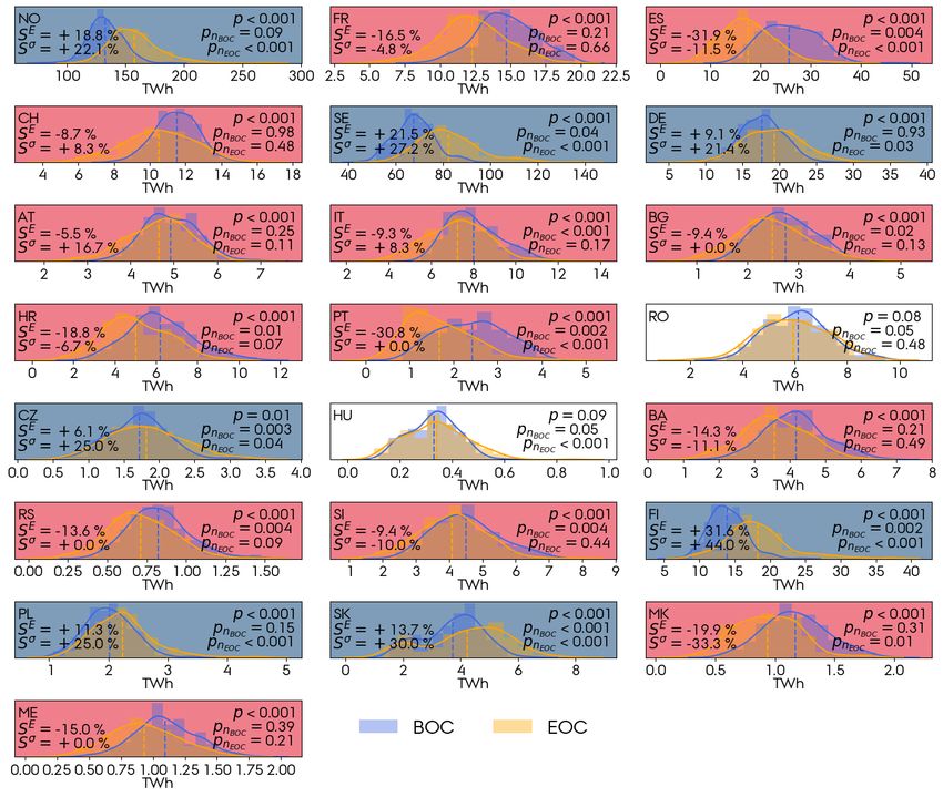
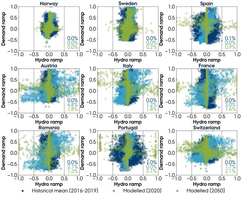
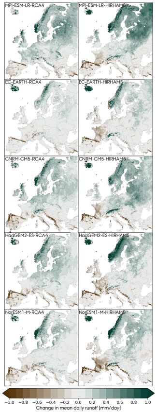
region in the USA. Future operation of hydropower also needs to consider that the
artificial flow fluctuations downstream of reservoirs caused by hydropeaking might
entail negative consequences for aquatic organisms [35].

Changes in hydropower inflow caused by climate change
As a prelude to this section, it is noteworthy that we are already witnessing climate
change impact on hydropower resources. Figure S17 presents simulated Norwegian
reservoir inflow, based on historical precipitation and temperature measurements,
from 1958 to 2017, produced by Holmqvist [36], and is a representation of the his-
torical climatic evolvement (energy capacity is assumed constant in the simulation).
A clear increasing trend in temperature and annual inflow can be observed.

As a preliminary step, we evaluate the absolute change in mean daily runoff at the
EOC period relative to the BOC (Eq. 1). Figure 5 shows the results for the combina-
tions of 5 GCMs and 2 RCMs for the RCP8.5 scenario. The signal is consistent for the
outer areas of the domain, i.e. runoff increases in northern Europe and decreases
in the south. The models vary in the magnitude and direction of change in some
regions. France is a good example of the latter: Runoff increases or shows negligi-
ble changes in combinations using RCA4 as RCM but decreases when HIRHAM5 is
used. The corresponding matrix of relative change in annual inflow (Eq. 2) derived
from the climate model runoff is presented in Figure 6. Consistently across models,
for the RCP8.5 scenario, Mediterranean countries show a significant reduction at the
EOC period while Nordic countries show a significant increase. When comparing the
runoff and inflow matrix, some considerations must be taken. First, the inflow ma-
trix is based on relative changes, which explains why e.g. Finland in some models
shows the largest increase in inflow when it is not reflected on the runoff. Second,
the modelled inflow is based on the location of the hydropower plants, see Figure
S6, and e.g. France has most of its plants located in the south, so the inflow is barely
affected by the runoff change in the north.

We now focus on analysing the intermodel and interannual variability. Figure 7 de-
picts the kernel density estimations of the probability density functions of the annual
inflow in Norway and Spain at the BOC and EOC 30-years periods for the 10 dif-
ferent climate models. As Figure 6 anticipates, the climate models all agree on an
increase in annual inflow in Norway and a reduction in Spain. The interannual vari-
ability, averaged for the 10 climate models, σ̄y , is projected to increase from 8.9% (of
the mean annual inflow) at the BOC period to 10.8% at the EOC in Norway, and de-
crease from 30.4% to 26.1% in Spain. The variability between the 10 climate model
(mean) projections, i.e. the intermodel variability σGCM-RCM is 7.5% for Norway and
13.7% for Spain at the EOC period (the intermodel variability at the BOC is zero due
to calibration with observed inflow). According to analysis of variance (ANOVA) [37],
since the variability between the 10 climate model projections, σGCM-RCM , is smaller
than the variability within, σ̄y , we can treat the 10 climate model projections at the
EOC as being from the same population. Based on that result, we group the 10
climate model projections into one ensemble consisting of 30 (years) x 10 (climate
models) observations. The variability contributed by changing the GCM or RCM is
examined in Supplementary Figure S16. It is shown that the range of the mean
annual inflow ĒEOC and the interannual variability σ̄y,EOC is generally larger when
varying the GCM than RCM. This result could indicate that the intermodel variability
is mainly due to the variation in the GCM, consistent with Christensen and Kjellström
[18]. However, to verify this indication, a larger number of RCMs would be needed.

Figure 8 shows the distributions of the annual inflow from the climate model ensem-
ble at the BOC and EOC periods (each consisting of 300 observations) for the 22
countries under analysis and the RCP8.5 scenario. First, a Shapiro-Wilk test [38]
is performed to check if the two sets are normally distributed, which is the case if
the probability score pnBOC and pnEOC are above 0.05. France, Switzerland, Austria,
Bosnia and Herzegovina, and Montenegro fulfil this condition. Second, a paired t-
test is conducted to check if we can reject the null hypothesis stating that the mean
difference between the two sets is zero. We apply it to every country, in spite of the

 7

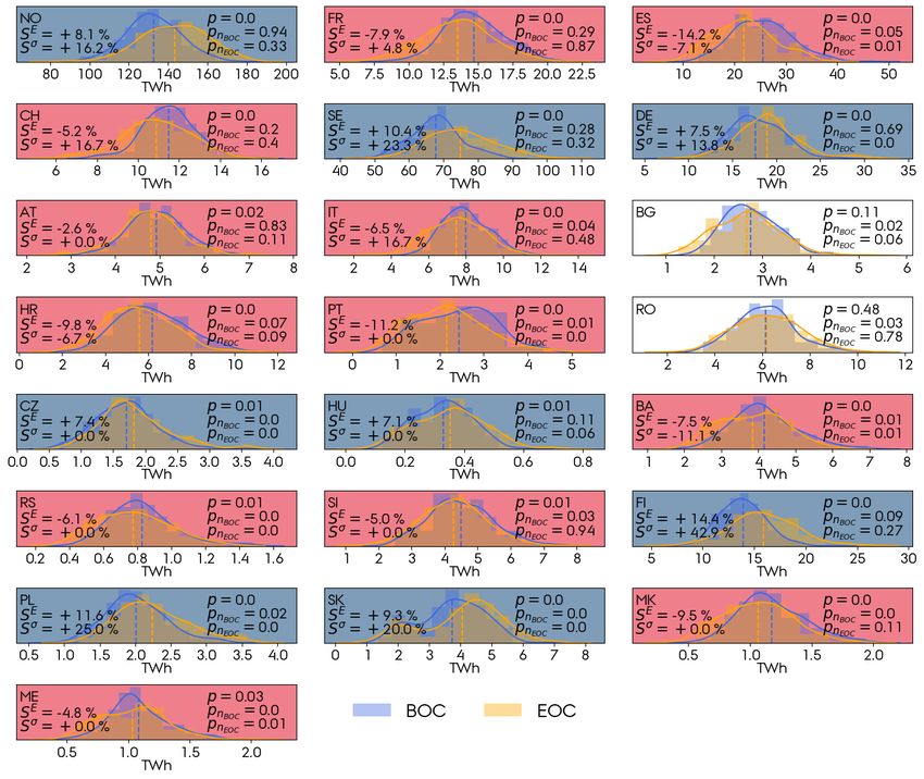
Figure 5: Change in mean
 daily runoff [mm/day] at the
 EOC period relative to the
 BOC for the RCP8.5
 scenario.

8

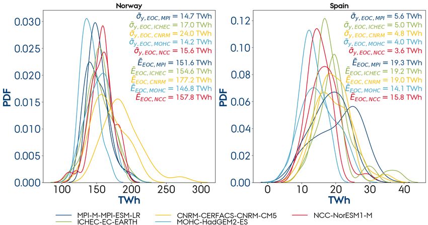
Figure 6: Relative changes
 in annual country-
 aggregated inflow at the
 EOC period relative to the
 BOC for the RCP8.5
 scenario.

9

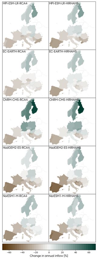
Figure 7: Kernel density estimations of the probability density functions for the annual inflow
 in Norway and Spain at the BOC (blue) and EOC (yellow) periods for the RCP8.5 scenario
with the corresponding interannual variability, σ̄y,BOC and σ̄y,EOC , and the intermodel variability
 at the EOC, σGCM-RCM,EOC .

indication from the Shapiro-Wilk test that some datasets are not normally distributed,
justified by all sets showing similar (bell-shaped) normal distribution characteristics.
The null hypothesis of zero difference between the EOC and BOC periods can be
rejected for all countries except Romania and Hungary. Figure 8 also shows the rela-
tive change in annual inflow S E and mean interannual variability S σy (normalised with
mean annual inflow). The latter is calculated for each model and averaged as in Fig-
ure 7, so S σ does not represent the width of the distributions plotted in Figure 8 since
they also include the intermodel variability. However, they might be similar since we
showed that the interannual variability is larger than the intermodel. Countries in
which annual inflow increases also show an enlarged interannual variability, that is,
countries that are expected to benefit from more abundant hydropower resources at
EOC will also suffer from stronger year-to-year fluctuations. Countries experiencing
a reduction in annual inflow do not show the same unanimity regarding the direction
of change of the interannual variability: The latter increases for countries in central
Europe (Switzerland, Austria, and Italy) but decreases in Mediterranean countries
(France, Spain, Croatia, Bosnia and Herzegovina, Slovenia, and North Macedonia).

The average of the signal from the 10 climate models, i.e. the ensemble mean, is
presented in Figure 9 in which the relative change in the annual inflow is indicated
on the map of Europe and the change in the seasonal inflow profile is given for the
countries with the largest hydropower capacity. The consequence of climate change
is latitude-dependent illustrated by the Northern European countries facing an in-
crease in the annual inflow while the Southern European countries, e.g. France,
Austria, Switzerland, and Italy, all encounter a scarcer annual resource available for
hydropower production. The most extreme impacts are found for Spain and Portu-
gal, 30% decrease in annual inflow under the RCP8.5 scenario, the Balkan countries
(10-20% decrease) and the Nordic countries (20-30% increase). All countries ex-
cept Spain are projected to encounter increased available hydro resources during
the winter since less water is stored as ice at high altitudes, but less during spring
and summer. Spain does not show any change in the shape of the seasonal profile
but it suffers from a reduced inflow throughout the year.

Thankfully, the RCP8.5 scenario has a low probability, given the current emissions
trends [39], but it is useful to look at it since it provides a more obvious signal. The
RCP4.5 scenario is, on the other hand, considered a likely scenario with current mit-
igation policies [39]. Figure 10 presents the box and whisker plots of the relative
change in annual inflow for the 22 countries at the three emissions scenarios (each
plot represents the distribution of 6x30, 8x30, and 10x30 model years for RCP2.6,
RCP4.5, and RCP8.5). When looking at the median (and other percentiles shown

 10

Figure 8: Ensemble distributions of the annual inflow at the BOC and EOC 30-years periods
for the RCP8.5 scenario. Dashed lines indicate the mean values of the distributions. The sets
 are normally distributed if pn > 0.05 based on a Shapiro-Wilk test. For the countries with a
statistically significant change (p < 0.05), a blue (red) shade indicates an increase (decrease)
 in the annual inflow. S E and S σ correspond to the relative change in annual inflow and
 interannual variability caused by climate change. For RCP4.5, see Figure S12.

by box and whiskers), the results are generally consistent in the direction of change
across the scenarios. For the RCP4.5 scenario, Spain and Portugal still show a
robust 11-14% decrease in annual inflow at the EOC period, the Balkan countries
(except Romania) show a 3-10% decrease, while the Nordic countries show a 8-
14% increase. For Romania, the impact diverges between a 1% increase and 3%
reduction across the RCP4.5 and RCP8.5.

Furthermore, we look at the frequency and severity of extreme events in inflow and
how they are impacted by climate change. We define droughts as consecutive days
with inflow 90th percentile. Figure 11 shows
the frequency and duration of inflow droughts in the different countries under the
RCP8.5 scenario (see Figure S15 for droughts under the RCP2.6 and RCP4.5 sce-
narios). Similarly, periods with overflow is shown in Figure S14. As hydropower
is expected to balance wind and solar fluctuations, severe droughts lasting several
weeks could stress the system operation. Unfortunately, for most countries, climate
change is expected to increase the length of drought periods and their frequency.
The observed tendency is stronger for Mediterranean countries. In addition, less
and shorter periods of overflow is expected in all countries, except Poland, Germany,
Czech Republic, Finland, and Slovakia.

As a final step, we investigate the impacts that the changes in inflow would have
on the coupled electricity and heating European energy system. To that end, we
compare the cost-optimal net-zero emissions system in 2050, when including the
climate projected hydro inflow time series at RCP8.5 (ensemble mean) at the BOC
and EOC periods. For those countries where significant changes in hydro resources
at the EOC period are expected, we find that the optimal wind and solar capacities
vary to compensate them, see Figure S18. However, the temporal patterns of hydro

 11

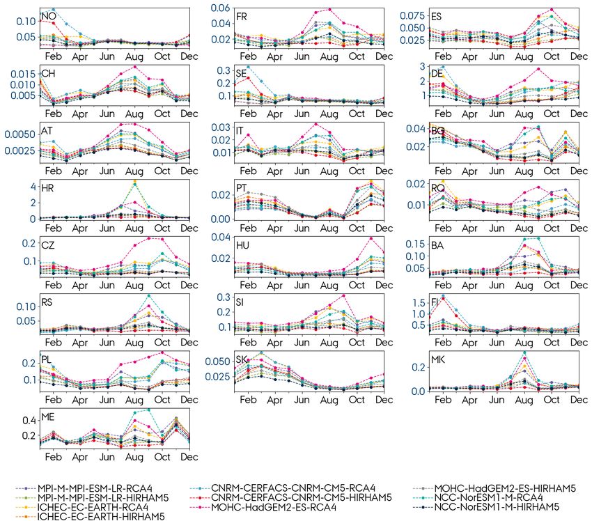
Figure 9: Ensemble mean relative change in annual inflow and change in seasonal inflow
profile for RCP8.5. Dashed patterns indicate results that are statistically significant (p

Figure 11: Duration and frequency of droughts, determined as consecutive days with inflow
less than the 10th percentile of inflow at the BOC, evaluated for the BOC and EOC periods
 under RCP8.5 scenario. For RCP2.6 and RCP4.5, see Figure S15, and for periods with
 overflow, see Figure S14.

CONCLUSION
In this work, we have investigated the impacts of climate change and high penetration
of wind and solar in the operation of reservoir hydropower plants in Europe. First, we
showed that balancing renewable generation requires increasing the seasonality of
hydropower operation. With the expected large solar capacities in Southern Europe,
hydropower plants located in this region are required to mostly operate during winter
and nighttime. The perfect foresight, typically assumed in energy models, implies
an optimal use of the hydropower balancing potential throughout the year. For most
countries, the new dispatch patterns seem possible, based on the historical opera-
tion. Higher frequency of large ramps is expected which can lead to reduced lifetime
of the hydropower plants. However, for countries with low reservoir energy capacity
and summer inflow peaks, e.g. Austria, Switzerland, and Italy, the hydropower dis-
patch shift from summer to winter, included in the model, may not be feasible.

Second, we showed that despite large interannual and significant intermodel varia-
tions, we can still detect a change in the inflow caused by climate change. For the
high emissions scenario (RCP8.5), using a paired t-test, we found a statistically sig-
nificant change in annual inflow at the EOC period, relative to BOC, for 20 out of 22
European countries under analysis. The ensemble mean relative change in annual
inflow is projected to decrease in Mediterranean and Balkan countries. Spain and
Portugal face the largest reduction: 31-32% for the high emissions scenario and 11-
14% for the mid (RCP4.5). Balkan countries (except Romania) face a reduction in
the range of 9-20% (3-10%) for the high (mid) emissions scenario. On top of that,
both regions will suffer from more frequent and prolonged droughts. Conversely, the
ensemble mean relative change in annual inflow is projected to increase in Northern
Europe. Annual inflow in Nordic countries increases in the range of 19-32% (8-14%)
for the high (mid) emissions scenario. The frequency of overflow events is expected
to increase for Finland but not for Sweden and Norway. The climate projections show
that climate change affect the interannual variability as well. Nordic countries, Ger-
many, Poland, and Slovakia robustly show a larger interannual variability under both
mid and high emissions, whereas for Switzerland, Italy, Spain, Bosnia and Herzegov-
ina, and Croatia it is reduced. When designing the future European energy system,
climate change impact on hydro resources will require additional wind and solar ca-
pacities in southern countries.

 13

SUPPLEMENTAL INFORMATION
Supplemental Information is found in Supplemental Materials.

ACKNOWLEDGEMENT
This work was authored by E.K.G and M.V., both funded by the RE-INVEST project
which is supported by the Innovation Fund Denmark under grant number 6154-
00022B.

AUTHOR CONTRIBUTIONS
Conceptualisation, M.V. and E.K.G.; project administration, visualization, and
writing−original draft, E.K.G.; writing−review & editing, E.K.G. and M.V.

DECLARATION OF INTERESTS
The authors declare no competing interests.

 14

REFERENCES

[1] COM. “Communication from the [10] Weber, J., Gotzens, F., and Witthaut, nents of mean climate and climate
 Commission to the European Par- D. “Impact of strong climate change change in a large ensemble of Euro-
 liament, the European Council, the on the statistics of wind power gen- pean regional climate model projec-
 Council, the European Economic and eration in Europe”. In: Energy Pro- tions”. In: Clim Dyn (2020), pp. 4293–
 Social Committee and the Committee cedia 153 (2018). 5th International 4308. DOI: 10 . 1007 / s00382 - 020 -
 of the Regions, The European Green Conference on Energy and Environ- 05229-y.
 Deal”. In: (2019). URL: https://eur- ment Research, ICEER 2018, 23-27
 lex . europa . eu / resource . html ? July 2018, Prague, Czech Republic, [19] Liu, H., Andresen, G. B., Brown, T.,
 uri=cellar:b828d165-1c22-11ea- pp. 22–28. ISSN: 1876-6102. DOI: 10. and Greiner, M. “A high-resolution hy-
 8c1f- 01aa75ed71a1.0002.02/DOC_ 1016/j.egypro.2018.10.004. dro power time-series model for en-
 1&format=PDF. ergy systems analysis: Validated with
 [11] Jerez, S., Tobin, I., and Vautard, Chinese hydro reservoirs”. In: Meth-
[2] Victoria, M., Zhu, K., Brown, T., An- R. et al. “The impact of climate odsX 6 (2019). DOI: 10.1016/j.mex.
 dresen, G. B., and Greiner, M. “Early change on photovoltaic power gen- 2019.05.024.
 decarbonisation of the European en- eration in Europe”. In: Nat Commun
 ergy system pays off”. In: Nature 6 (2015), p. 10014. DOI: 10 . 1038 / [20] Giorgi, F., Jones, C., and Asrar,
 Communications (2020). DOI: 10 . ncomms10014. G.R. “Addressing climate informa-
 1038/s41467-020-20015-4. tion needs at the regional level: the
 [12] Fonseca, F. R. et al. “Effects of Cli- CORDEX framework”. In: WMO Bul-
[3] IEA. IEA Databrowser. International mate Change on Capacity Expansion letin 58 (2009), pp. 175–183.
 Energy Agency. URL: https : / / Decisions of an Electricity Genera-
 www . iea . org / fuels - and - tion Fleet in the Southeast U.S.” In: [21] JRC. JRC Hydro-power database.
 technologies/electricity#data- Environ. Sci. Technol. 55, 4 (2021), European Commission, Joint Re-
 browser. pp. 2522–2531. DOI: 10.1021/acs. search Centre. 2019. URL: https :
 est.0c06547. / / data . jrc . ec . europa . eu /
[4] Pfeiffer, O., Nock, D., and Baker, dataset / 52b00441 - d3e0 - 44e0 -
 E. “Wind energy’s bycatch: Offshore [13] Lehner, B., Czisch, G., and Vas- 8281-fda86a63546d.
 wind deployment impacts on hy- solo, S. “The impact of global change
 dropower operation and migratory on the hydropower potential of Eu- [22] Lehner, B. and Grill, G. “Global
 fish”. In: Renewable and Sustain- rope: a model-based analysis”. In: river hydrography and network rout-
 able Energy Reviews 143 (2021), Energy Policy 33.7 (2005), pp. 839– ing: baseline data and new ap-
 p. 110885. ISSN: 1364-0321. DOI: 10. 855. ISSN: 0301-4215. DOI: https:// proaches to study the world’s large
 1016/j.rser.2021.110885. doi.org/10.1016/j.enpol.2003. river systems”. In: Hydrological Pro-
 10.018. cesses, 27(15): 2171–2186 (2013).
[5] Sterl, S., Fadly, D., Liersch, S., Koch, URL: https : / / hydrosheds . org /
 H., and Thiery, W. “Linking solar and [14] Turner, S. W. D., Ng, J. Y., and Galelli, page/hydrobasins.
 wind power in eastern Africa with op- S. “Examining global electricity sup-
 eration of the Grand Ethiopian Re- ply vulnerability to climate change us- [23] ATLITE. Convert weather data to en-
 naissance Dam”. In: Nature Energy ing a high-fidelity hydropower dam ergy systems data. URL: https : / /
 (2021). DOI: 10.1038/s41560- 021- model”. In: Science of the Total En- atlite . readthedocs . io / en /
 00799-5. vironment (2017), pp. 663–675. DOI: latest/ (visited on 09/03/2021).
 10 . 1016 / j . scitotenv . 2017 . 03 .
[6] Cronin, J., Anandarajah, G., and 022.
 [24] WCRP. CORDEX database. URL:
 Dessens, O. “Climate change im- https : / / esgf - data . dkrz . de /
 pacts on the energy system: a re- [15] Van Vliet, M. T. H., Wiberg, D., Leduc, search/cordex-dkrz/.
 view of trends and gaps”. In: Climatic S., and Riahi, K. “Power-generation
 Change 151 (2018), pp. 79–93. DOI: system vulnerability and adaptation
 [25] Pachauri, R.K. and Meyer,
 10.1007/s10584-018-2265-4. to changes in climate and water re-
 L.A. Meyer. Climate Change 2014:
 sources”. In: Nature Climate Change
 Synthesis Report. Contribution of
[7] Yalew, S.G., Vliet, M.T.H. van, and 6 (2016), pp. 375–380. DOI: 10 .
 Working Groups I, II and III to the
 Gernaat, D.E.H.J. et al. “Impacts of 1038/nclimate2903.
 Fifth Assessment Report of the
 climate change on energy systems Intergovernmental Panel on Cli-
 in global and regional scenarios”. In: [16] Van Vliet, M. T. H., Vögele, S., and mate Change. 2020, p. 151. URL:
 Nat Energy 5 (2020), pp. 794–802. Rübbelke, D. “Water constraints on https : / / ar5 - syr . ipcc . ch /
 DOI : 10.1038/s41560-020-0664-z. European power supply under cli- ipcc / ipcc / resources / pdf / IPCC _
 mate change: impacts on electricity SynthesisReport.pdf.
[8] EEA. Adaptation challenges and op- prices”. In: Environmental Research
 portunities for the European energy Letters (2013). DOI: 10.1088/1748-
 [26] Giorgetta, M. A. et al. “Climate and
 system. 2019. URL: https : / / www . 9326/8/3/035010.
 carbon cycle changes from 1850 to
 eea . europa . eu / publications / 2100 in MPI-ESM simulations for
 adaptation-in-energy-system. [17] Schaefli, B., Hingray, B., and Musy, the Coupled Model Intercomparison
 A. “Climate change and hydropower Project phase 5”. In: Journal of Ad-
[9] Schlott, M., Kies, A., Brown, T., production in the Swiss Alps: quan- vances in Modeling Earth Systems
 Schramm, S., and Greiner, M. “The tification of potential impacts and re- 5.3 (2013), pp. 572–597. DOI: https:
 impact of climate change on a cost- lated modelling uncertainties”. In: Hy- //doi.org/10.1002/jame.20038.
 optimal highly renewable European drol. Earth Syst. Sci. 11(3) (2007),
 electricity network”. In: Applied En- pp. 1191–1205. DOI: 10.5194/hess-
 [27] Hazeleger, W. et al. “EC-Earth V2.2:
 ergy (2018). DOI: 10 . 1016 / j . 11-1191-2007.
 description and validation of a new
 apenergy.2018.09.084. seamless earth system prediction
 [18] Christensen, O. B. and Kjellström, model”. In: Climate Dynamics (2012),
 E. “Partitioning uncertainty compo-

 15

pp. 2611–2629. DOI: 10 . 1007 / Rossby Centre Regional Climate [35] Schmutz, S. and Sendzimir, J. River-
 s00382-011-1228-5. model RCA3: model description and ine Ecosystem Management. Vol. 8.
 performance”. In: Tellus A: Dynamic Springer, 2018. DOI: 10.1007/978-
[28] Voloire, A. et al. “The CNRM-CM5.1 Meteorology and Oceanography 63.1 3-319-73250-3.
 global climate model: description and (2011), pp. 4–23. DOI: 10 . 1111 / j .
 basic evaluation”. In: Climate Dynam- 1600-0870.2010.00478.x. [36] Holmqvist, E. Norges vannbalanse i
 ics (2013), pp. 2091–2121. DOI: 10. TWh basert påHBV-modeller. 2017.
 1007/s00382-011-1259-y. [32] Bøssing Christensen, O., Drews, M., URL : https://publikasjoner.nve.
 Hesselbjerg Christensen, J., Dethloff, no / rapport / 2017 / rapport2017 _
[29] Collins, W. J. et al. “Development and K., Ketelsen, K., Hebestadt, I., and 87.pdf.
 evaluation of an Earth-System model Rinke, A. The HIRHAM Regional Cli-
 – HadGEM2”. In: Geoscientific Model mate Model. Version 5 (beta). En- [37] Weiss, D. J. Analysis of Variance and
 Development 4.4 (2011), pp. 1051– glish. Denmark. Danish Meteorolog- Functional Measurement : A Practi-
 1075. DOI: 10 . 5194 / gmd - 4 - 1051 - ical Institute. Technical Report 06-17. cal Guide. 1st ed. Oxford University
 2011. Danish Climate Centre, Danish Mete- Press, Incorporated, 2005.
 orological Institute, 2007.
[30] Bentsen, M. et al. “The Norwegian [38] SHAPIRO, S. S. and WILK, M. B. “An
 Earth System Model, NorESM1-M – [33] Bakken, B. H. and Bjorkvoll, T. “Hy- analysis of variance test for normality
 Part 1: Description and basic eval- dropower unit start-up costs”. In: (complete samples)”. In: Biometrika
 uation of the physical climate”. In: IEEE Power Engineering Society 52 (3-4 1965), pp. 591–611. DOI: 10.
 Geoscientific Model Development 6.3 Summer Meeting (2002). DOI: 10 . 1093/biomet/52.3-4.591.
 (2013), pp. 687–720. DOI: 10.5194/ 1109/PESS.2002.1043646.
 gmd-6-687-2013. [39] Hausfather, Z. and Peters, G. P.
 [34] Gallego-Castillo, C. and Victoria, M. “Emissions – the ‘business as usual’
[31] Samuelsson, P., Jones, C. G., WillEn, “Improving Energy Transition Anal- story is misleading”. In: Nature 577
 U., Ullerstig, A., Gollvik, S., Hans- ysis Tool through Hydropower Sta- (2020), pp. 618–620. DOI: 10.1038/
 son, U., Jansson, E., KjellstroM, C., tistical Modelling”. In: Energies 14.1 d41586-020-00177-3.
 Nikulin, G., and Wyser, K. “The (2021). ISSN: 1996-1073. DOI: 10 .
 3390/en14010098.

 16

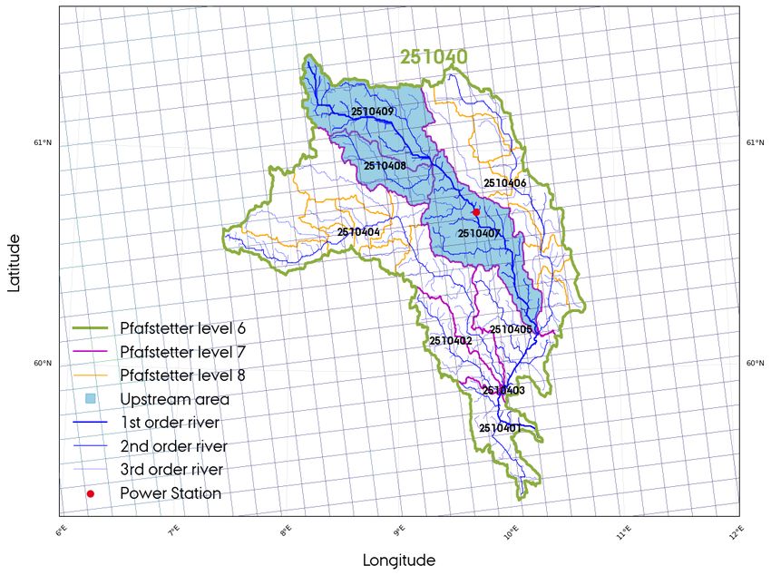
Supplementary material

S1 Methods
Upstream determination
Surface runoff is the excess water from precipitation, i.e. rain and snow, or meltwater
from snow or glaciers that does not enter the soil (infiltration) or evaporates into the
atmosphere. The runoff movement is actuated by gravity, and the flow direction is
determined by the topography, i.e. the shape of the land surface. The runoff will
eventually reach a river, a lake, a pond etc. and be collected in here. A drainage
basin (referred to as basin) is the area of land that drains all flow of water, e.g.
runoff, river streams, groundwater etc., to a common outlet, e.g. a river, reservoir,
the ocean etc. [1]. The basins can be delineated from topographic maps, using
the Pfafstetter coding scheme from Verdin and Verdin [2]. The Pfafstetter code itself
indicates the number of subdivisions and the basin type. If the last digit is odd the
basin is an interbassin meaning that the main stem of the river runs through it. If the
last digit is even, the basin is a tributary basin and only has tributaries connecting to
the river. Finally, if the last digit is zero, it is an isolated internal basin that does not
have any river connections with surrounding basins. Increasing the level, increases
the resolution, thus the size of each basin is reduced. By this approach, one digit is
added to the Pfafstetter code, e.g. a level 1 code has one digit, level 2 has two digits,
etc. The amount of runoff that is caught by the river does not only depend on the
runoff in one single subbasin, but does, due to the interconnection, also depend on
the runoff collected by the river-connecting basins. The basin area that contributes
to the runoff in a reservoir, is termed as the upstream area.

 2510409 2510408
 (2070220570) (2070220690)
 [2510407] [2510407]

 2510407 2510406
 (2070231400) (2070231370)
 [2510405] [2510405]

 2510405
 2510404
 (2070235180)
 (2070235170)
 [2510403]
 [2510403]

 2510403 2510402
 (2070235660) (2070235650)
 [2510401] [2510401]

 2510401
 (2070033670)
 [0]

Figure S1: Tree of the level 7 basins connection in one river system in Norway. Numbers are
Pfafstetter codes representing each subbasin. In paranthesis the unique basin identifier from
the hydroBASINS database is given, and square brackets indicate the Pfafstetter code of the
 basin into where the river flows, i.e. the next downstream basin, with zero indicating the
 mouth of the river.

Figure S2 considers one particular power station located in basin 2510407, in South-
ern Norway. By looking at the network in Figure S1, it is known that basin 2510408
(tributary) and 2510409 (interbasin) contribute to the flow in basin 2510407, and they
all constitute the upstream area for the reservoirs in this specific basin. The upstream
determination was in this case based on a Pfafstetter level 7 delineation.

As Figure S2 also shows, the resolution of the delineation is refined with Pfafstetter
level 8. Liu et al. [3] applied level 7 at a 0.3◦ × 0.3◦ runoff grid. In this work, the runoff
data is acuired at a 0.11◦ × 0.11◦ . In line with this refinement, we determine the
upstream basins based on a level 8 basins delineation. A preliminary study shows
that in 15 countries countries, level 8 leads to a higher correlation between modelled
and historical inflow, shown in Figure S3.

 17

Figure S2: Upstream area depiction of one power plant in Norway, using a level 7 basin
 delineation, with an overlay of the EURO-CORDEX EUR-11 grid.

Figure S3: Pearson correlation between modelled (MPI-ESM-LR-RCA4) and historical inflow
at Pfafstetter level 7 and 8 basins delineation. Slovakia is excluded from this figure since it is
 negative in both cases.

Runoff aggregation
Using the distance between the runoff grid cell and the reservoir, and assuming
a flow speed of 1 m/s, the runoff is first aggregated in the basins connected to a
reservoir, followed by a country-level aggregation and conversion into a volumetric
flow rate. Country-aggregated volumetric inflow is calculated with Eq. 3:
 M
 X Rbc Ab
 Qc = , (3)
 ∆t
 b

where b is the upstream basin index, M is the number of upstream basins within
country c, Rbc is the aggregated runoff in basin b and country c [m], Ab is the surface

 18

area of the basin [m2 ], ∆t is the temporal resolution of the runoff data [s], and Qc is
the country-aggregated volumetric inflow [m3 /s].

Energy conversion
The aggregated volumetric inflow can be transformed into units of energy to make it
comparable with historical inflow. Figure S4 shows a simple illustration of one grid
cell i containing runoff at the altitude zi . Assuming that the initial velocity of the
runoff is zero, i.e. negligible kinetic energy, the maximum theoretically extractable
energy E max (per time step) of the runoff at altitude zi by the turbine at altitude zT is
estimated with Eq. 4:
 E max = ηρgQ(zi − zT )∆t , (4)
where η is the turbine efficiency which is assumed to be 1, g is the gravitational
acceleration (9.81 m/s2 ), ρ is the water density (1000 kg/m3 ), and Q is the flow rate
of the runoff. In reality, some of the potential energy of the water in the grid cell is
converted into kinetic energy when moving down the terrain and subsequently lost
when reaching the reservoir; thus, the available energy E available is reduced to:

 E available = ρgQ(zR − zT )∆t = ρgQH∆t , (5)

where zR is the altitude of the hydropower reservoir and H is the (hydraulic) head.
Note that for run-of-river power plants the kinetic energy would not be lost, since this
type of plant extracts the kinetic energy directly.

 Mountain

 Runoff grid cell 

 Reservoir

 Dam
 
 Turbine

 Sea level 0 = 0

Figure S4: Simplified illustration of one runoff grid cell connected to a hydropower reservoir.

 PN
In Eq. 3, we rewrite Rbc = i Ribc , where N is the number of grid cells within one
basin. Furthermore, we approximate the head in Eq. 5 by altitude zi , due to the lack
of data on reservoir head of every existing hydropower plant, which yields:
 M X
 X N
 Ecmodel = ρg zi Ribc Ab , (6)
 b i

where Ecmodel is the contry-aggregated modelled energy inflow. The head approxi-
mation leads to the error ez caused by the mismatch between the altitude zi and the
reservoir head H:
 ez = zi − H (7)
The bias caused by the mismatch will be adjusted in the calibration with the retain
factor, described in the following section.

 19

Retain factor
The retain factor RF quantifies the level of water lost due to evaporation, transpira-
tion, irrigation, or groundwater infiltration, contributing to an energy loss E loss , and is
determined for each country based on the seasonal profile obtained from the mod-
elled inflow at the beginning of the century (1991-2020) and the historical observa-
tions (2016-2019) by:
 hist
 Observed inflow Ecm
 RFcm = = model , (8)
 Modelled inflow at BOC Ecm

where index c indicates country (1-22) and m month of an average year (1-12).
According to the definition presented in Eq. 8, RF corresponds to the fraction of
upstream-runoff caught by the hydropower reservoirs, i.e. the retained water. The
retain factor includes the bias correction for the mismatch between the head and the
runoff altitude, e¯z . Evaporation taking place while water is stored in the reservoir can
also impact the potential power generation [4]. The retain factor also accounts for
this.

The model performance is, prior to calibration with the retain factor, evaluated on the
Pearson correlation betwen modelled and observed inflow:
 P12
 m=1 (Êm − hÊi)(Em − hEi)
 rÊE = qP qP , (9)
 12 2) 12 2
 m=1 ( Êm − h Êi m=1 (E m − hEi)

where Êt is the modelled inflow at month m, hÊi is the modelled mean inflow, Em is
the observed inflow at month m, and hEi is the observation mean inflow.

The modelled inflow for both BOC and EOC is calibrated with the retain factor:
 M X
 X N
 calibrated
 Ecm = RFcm (E loss , e¯z )Ecm
 model
 = RFcm (E loss , e¯z )ρg zi Ribc Ab (10)
 b i

By using Eq. 10 for the calibration of inflow at EOC, we assume that climate change
does not affect the seasonality and magnitude of the retain factor. In reality, the global
temperature rise is accompanied by a larger evaporation rate, which increases the
energy loss. This is not accounted for in our approach.

S2 Data
Historical inflow and dispatch
The European Network of Transmission System Operators for Electricity (ENTSO-E)
Transparency Platform [5] provides hourly hydropower generation and weekly reser-
voir filling level. Using an energy balance, the weekly reservoir filling level can be
expressed as:
 168
 X
 loss
 Vw+1 = Vw + Ew − Gh − Ew (11)
 h=1

where Vw is the reservoir filling level at week w, Vw+1 the same at week w + 1,
 loss
Ew is the energy inflow, Gh is the electricity generation at hour h, and Ew is the
energy loss. By collecting hourly electricity generation and weekly reservoir filling
level at ENTSO-E and neglecting the energy loss, the weekly energy inflow Ew is
approximated with Eq. 11. The validity of this approximation is evaluated for Nor-
way and Spain by comparing the approximated inflow with historical inflow from The
Norwegian Water Resources and Energy Directorate (NVE) [6] and Red Eléctrica
De España (REE) [7]. The comparison is illustrated in Figure S5 which shows good
coherence.

Data from ENTSO-E is available for Austria, Bulgaria, France, Italy, Portugal, Ro-
mania, Switzerland, Montenegro, Norway, Spain, and Sweden with a period ranging

 20

Norway Spain

 30 8

 25 6
Inflow [TWh]

 Inflow [TWh]
 20
 15 4

 10 2
 5
 0
 Jun Oct Jun Oct Jun Oct Jun Oct Jun Oct Jun Oct
 2016 2017 2016 2017 2018 2019
 NVE ENTSO-E REE
 Figure S5: Inflow approximated from electricity generation and reservoir filling level data from
 ENTSO-E compared with historical inflow from NVE (Norway) and REE (Spain).

 from 2016 to 2019. Countries such as Norway, Spain, and Sweden have a wider
 time range of historical inflow available through NVE [6] (1958-2017), REE [7] (1990-
 2019), and Swedenergy [8] (1980-2019), which are used instead of ENTSO-E. His-
 torical data for the remaining countries which are not available at ENTSO-E, i.e.
 Bosnia-Herzegovina, Croatia, Czech Republic, Finland, Germany, Poland, Serbia,
 Slovakia, Slovenia, Hungary, and North Macedonia is provided by Wattsight [9], but
 will not be openly available. For the dispatch intraday and seasonal profile com-
 parison in Figure 3 and S7, the historical data is based on hourly reservoir and
 run-of-river hydropower generation from ENTSO-E. To analyse the dispatch-inflow
 correlation in Figure 4 and S8a, and the ramp rate in Figure S9, weekly reservoir
 inflow derived from ENTSO-E reservoir dispatch and filling level is compared with
 ENTSO-E reservoir dispatch.

 Modelled dispatch
 Modelled dispatch is acquired from the hourly-resolved sector-coupled network model
 of the European energy system consisting of 30 nodes from Victoria et al. [10] before
 (2020) and after decarbonisation (2050). A key characteristic of the model is that it
 assumes a perfect foresight, which implies that electricity consumption and the inflow
 is known one year forward. The perfect foresight enables the system to optimize the
 usage of hydropower, and the water in the reservoirs is thus only released when it is
 cost-optimal for the system.

 Climate model data
 Climate model data is acquired from regional climate models available at ESGF
 [11] given with a combination of 5 GCMs (MPI-M-MPI-ESM-LR[12], ICHEC-EC-
 EARTH[13], CNRM-CERFACS-CM5[14], MOHC-HadGEM2-ES[15], and
 NCC-NorESM1-M[16]) and 2 RCMs (RCA4[17] and HIRHAM5[18]). Each climate
 model is of 0.11◦ × 0.11◦ horisontal and daily resolution and data is acquired for
 the BOC (1991-2020) and EOC (2071-2100) periods. Some climate models are
 subject to different calendar systems. E.g. NorESM1-M does not include leap years
 and HadGEM2-ES uses a 360 days per year calendar with 30 days in each month.
 Furthermore, HadGEM2-ES does not include the year 2100, and, thus, only 29 years
 will describe the EOC period with this GCM. In these irregular situations, the missing
 days will be filled out by repeating the data of the previous day, month or year.

 21

Location of hydropower plants
Locations of hydropower plants are collected from the JRC Hydropower Database
[19]. The location and power capacities from the database for the 22 considered
countries are illustrated in Figure S6.

 Figure S6: Location and power capacities of reservoirs (res.), pumped-hydro storages
 (pump.), and run-of-river (r.o.r) power plants from JRC [19].

Basins delineation
The boundaries of the watersheds, i.e. the basins delineations, are collected from
the HydroBASINS [20] with Pfafstetter level 8.

 22

S3 Results

 Norway 12 Sweden Spain
 24
 22 10 7
 Dispatch [GWh]

 Dispatch [GWh]

 Dispatch [GWh]
 20 6
 18 8 5
 16 4
 14 6 3
 12 4 2
 10 1
 0 4 8 12 16 20 0 4 8 12 16 20 0 4 8 12 16 20
 Austria Italy France
 5.5 9 10
 5.0 8
 Dispatch [GWh]

 Dispatch [GWh]

 Dispatch [GWh]
 4.5 7 8
 4.0 6
 3.5 5 6
 3.0 4
 2.5 3 4
 2
 2.0 10 4 8 12 16 20 2
 0 4 8 12 16 20 0 4 8 12 16 20
 Romania Portugal Switzerland
 3.0 2.5 7
 Dispatch [GWh]

 Dispatch [GWh]

 Dispatch [GWh]
 2.5 2.0 6
 5
 2.0 1.5 4
 1.5 1.0 3
 0.5 2
 1.0 1
 0.0
 0 4 8 12 16 20 0 4 8 12 16 20 0 4 8 12 16 20
 hour hour hour
 Modelled (2020) Historical mean (2016-2019)
 Modelled (2050) Historical range (2016-2019)
 (a)
 Norway Sweden 8 Spain
 18 8 7
 Dispatch [TWh]

 Dispatch [TWh]

 Dispatch [TWh]

 16 7 6
 14 6 5
 12 4
 10 5 3
 8 4 2
 1
 6 3 0
 Feb Apr Jun Aug Oct Dec Feb Apr Jun Aug Oct Dec Feb Apr Jun Aug Oct Dec
 Austria Italy 12 France
 3.5 6 10
 Dispatch [TWh]

 Dispatch [TWh]

 Dispatch [TWh]

 3.0 5 8
 2.5 4 6
 2.0 3 4
 1.5 2 2
 Feb Apr Jun Aug Oct Dec 1 Feb Apr Jun Aug Oct Dec Feb Apr Jun Aug Oct Dec
 Romania Portugal Switzerland
 3.5 5
 2.5 3.0
 Dispatch [TWh]

 Dispatch [TWh]

 Dispatch [TWh]

 2.0 2.5 4
 1.5 2.0 3
 1.5
 1.0 1.0 2
 0.5 0.5 1
 0.0
 Feb Apr Jun Aug Oct Dec Feb Apr Jun Aug Oct Dec Feb Apr Jun Aug Oct Dec
 Modelled (2020) Historical mean (2016-2019)
 Modelled (2050) Historical range (2016-2019)
 (b)

Figure S7: Supplemental to Figure 3: Modelled and historical (a) intraday and (b) seasonal
 operation of hydropower plants.

 23

Norway Sweden Spain
 10 r = -0.58 6 r = -0.2 2.0 r = 0.82
 8 p = 1.6e-05 5 p = 1.7e-01 p = 6.2e-13
 4 1.5
 6
 [TWh]

 [TWh]

 [TWh]
 3 1.0
 4 2
 2 1 0.5
 0 0 0.0
 2016 2017 2018 2019 2016 2017 2018 2019 2016 2017 2018 2019
 0.40 Austria Italy France
 r = 0.84 1.75 r = 0.45 0.7 r = 0.48
 0.35 p = 5.3e-14 1.50 p = 1.3e-03
 0.30 0.6 p = 5.3e-04
 1.25 0.5
 0.25 1.00
[TWh]

 [TWh]

 [TWh]
 0.20 0.4
 0.15 0.75 0.3
 0.10 0.50
 0.25 0.2
 0.05 0.1
 0.00 0.00
 2016 2017 2018 2019 2016 2017 2018 2019 2016 2017 2018 2019
 Romania Portugal Switzerland
 0.5 r = 0.69 1.4 r = 0.52
 0.4 r = 0.45
 p = 1.2e-03 0.4 p = 1.1e-07 1.2 p = 2.3e-04
 0.3 1.0
 0.3 0.8
 [TWh]

 [TWh]

 [TWh]
 0.2 0.2 0.6
 0.1 0.4
 0.1 0.2
 0.0 0.0 0.0
 2016 2017 2018 2019 2016 2017 2018 2019 2016 2017 2018 2019
 Inflow Dispatch
 (a)
 AT ES
 0.8 PT
 r = -0.844, p = 0.004
 0.6
 Pearson correlation

 CH
 ITFR RO
 0.4 IT
 0.2
 0.0
 0.2 SE

 0.4
 NO
 0.6
 500 1000 1500 2000 2500 3000
 Discharge time [h]
 (b)

Figure S8: Supplemental to Figure 4: (a) Historical hydropower reservoir inflow and dispatch
 from 2016 to 2019 from ENTSO-E (thin lines indicate weekly values and thick monthly
averaged), and (b) inflow-dispatch correlation and discharge time. In (a) Pearson correlation
 r represents the correlation between inflow and dispatch, and in (b) r represents the
correlation between the inflow-dispatch correlation and the discharge time. Furthermore, p is
 the statistical significance of the Pearson correlation.

 24