ProMove mini Wireless Inertial Sensing Platform - User Manual v3.8.8 - Inertia Technology
←
→
Page content transcription
If your browser does not render page correctly, please read the page content below
ProMove‐mini
Wireless Inertial Sensing Platform

            User Manual
               v3.8.8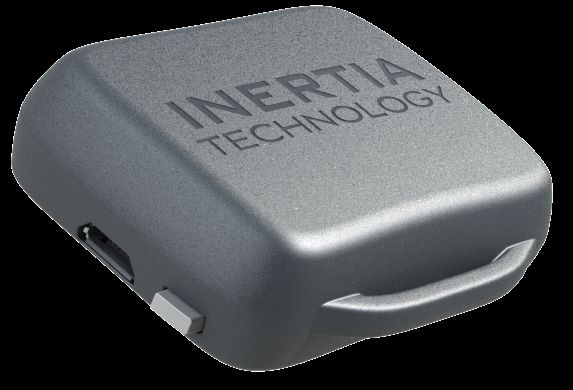
Contents
1 Introduction                                                                                                                                          5

2 Safety Instructions                                                                                                                                   6

3 Setup                                                                                                                                                  7
  3.1 System Description . . .      .   .   .   .   .   .   .   .   .   .   .   .   .   .   .   .   .   .   .   .   .   .   .   .   .   .   .   .   .    7
  3.2 Gateway Connections . .       .   .   .   .   .   .   .   .   .   .   .   .   .   .   .   .   .   .   .   .   .   .   .   .   .   .   .   .   .    8
  3.3 Node LEDs and Button .        .   .   .   .   .   .   .   .   .   .   .   .   .   .   .   .   .   .   .   .   .   .   .   .   .   .   .   .   .    9
  3.4 Attachments . . . . . . .     .   .   .   .   .   .   .   .   .   .   .   .   .   .   .   .   .   .   .   .   .   .   .   .   .   .   .   .   .    9
  3.5 Recharging the Batteries      .   .   .   .   .   .   .   .   .   .   .   .   .   .   .   .   .   .   .   .   .   .   .   .   .   .   .   .   .   10
  3.6 On‐board Storage . . . .      .   .   .   .   .   .   .   .   .   .   .   .   .   .   .   .   .   .   .   .   .   .   .   .   .   .   .   .   .   10

4 Inertia Studio                                                                                                                                        11
  4.1 Main Screen . . . . . . . . . . . . . . . . . . . .                               .   .   .   .   .   .   .   .   .   .   .   .   .   .   .   .   11
        4.1.1 Toolbar and Menu . . . . . . . . . . . .                                  .   .   .   .   .   .   .   .   .   .   .   .   .   .   .   .   12
        4.1.2 Plots . . . . . . . . . . . . . . . . . . . .                             .   .   .   .   .   .   .   .   .   .   .   .   .   .   .   .   14
        4.1.3 Information Area . . . . . . . . . . . . .                                .   .   .   .   .   .   .   .   .   .   .   .   .   .   .   .   15
  4.2 Connecting to a Device . . . . . . . . . . . . . .                                .   .   .   .   .   .   .   .   .   .   .   .   .   .   .   .   17
        4.2.1 Connecting to a Device Using the Toolbar                                  .   .   .   .   .   .   .   .   .   .   .   .   .   .   .   .   17
        4.2.2 Connecting to a Device Using the Menu .                                   .   .   .   .   .   .   .   .   .   .   .   .   .   .   .   .   17
  4.3 Logging to File . . . . . . . . . . . . . . . . . . .                             .   .   .   .   .   .   .   .   .   .   .   .   .   .   .   .   19
  4.4 Logging to Flash . . . . . . . . . . . . . . . . . .                              .   .   .   .   .   .   .   .   .   .   .   .   .   .   .   .   21
        4.4.1 Starting and Stopping a Flash Log . . . .                                 .   .   .   .   .   .   .   .   .   .   .   .   .   .   .   .   21
        4.4.2 Downloading a Flash Log . . . . . . . . .                                 .   .   .   .   .   .   .   .   .   .   .   .   .   .   .   .   22
        4.4.3 Deleting Flash Logs . . . . . . . . . . . .                               .   .   .   .   .   .   .   .   .   .   .   .   .   .   .   .   23
  4.5 Filling in Lost Samples . . . . . . . . . . . . . . .                             .   .   .   .   .   .   .   .   .   .   .   .   .   .   .   .   24
        4.5.1 Automatic . . . . . . . . . . . . . . . . .                               .   .   .   .   .   .   .   .   .   .   .   .   .   .   .   .   24
        4.5.2 Manual . . . . . . . . . . . . . . . . . .                                .   .   .   .   .   .   .   .   .   .   .   .   .   .   .   .   25
        4.5.3 Details . . . . . . . . . . . . . . . . . . .                             .   .   .   .   .   .   .   .   .   .   .   .   .   .   .   .   25
  4.6 Exporting a Logfile . . . . . . . . . . . . . . . .                               .   .   .   .   .   .   .   .   .   .   .   .   .   .   .   .   27
        4.6.1 CSV Settings . . . . . . . . . . . . . . . .                              .   .   .   .   .   .   .   .   .   .   .   .   .   .   .   .   28
        4.6.2 MAT Settings . . . . . . . . . . . . . . .                                .   .   .   .   .   .   .   .   .   .   .   .   .   .   .   .   29
        4.6.3 Visual3D Settings . . . . . . . . . . . . .                               .   .   .   .   .   .   .   .   .   .   .   .   .   .   .   .   30
  4.7 Replaying a Logfile . . . . . . . . . . . . . . . .                               .   .   .   .   .   .   .   .   .   .   .   .   .   .   .   .   31
        4.7.1 Real‐Time . . . . . . . . . . . . . . . . .                               .   .   .   .   .   .   .   .   .   .   .   .   .   .   .   .   31
        4.7.2 Analysis . . . . . . . . . . . . . . . . . .                              .   .   .   .   .   .   .   .   .   .   .   .   .   .   .   .   32
  4.8 Configuring the Sensors . . . . . . . . . . . . . .                               .   .   .   .   .   .   .   .   .   .   .   .   .   .   .   .   33
        4.8.1 Global Settings . . . . . . . . . . . . . .                               .   .   .   .   .   .   .   .   .   .   .   .   .   .   .   .   34
        4.8.2 Accelerometer Settings . . . . . . . . . .                                .   .   .   .   .   .   .   .   .   .   .   .   .   .   .   .   36
        4.8.3 Compass Settings . . . . . . . . . . . . .                                .   .   .   .   .   .   .   .   .   .   .   .   .   .   .   .   37

inertia‐technology.com                                                                                                                  Page 2 of 71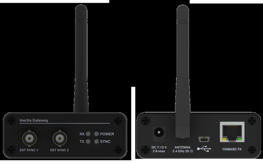
4.8.4 Gyroscope Settings . . . . . . . . . . . . . . . . . . . . . . . . . . . . 38
4.8.5 Barometer Settings . . . . . . . . . . . . . . . . . . . . . . . . . . . . 39
4.8.6 High‐G Accelerometer Settings . . . . . . . . . . . . . . . . . . . . . . 40
4.8.7 Temperature Settings . . . . . . . . . . . . . . . . . . . . . . . . . . . 41
4.8.8 IMA Settings . . . . . . . . . . . . . . . . . . . . . . . . . . . . . . . 42
4.8.9 RTC Settings . . . . . . . . . . . . . . . . . . . . . . . . . . . . . . . . 43
4.8.10 GNSS Settings . . . . . . . . . . . . . . . . . . . . . . . . . . . . . . . 44
4.8.11 Status Settings . . . . . . . . . . . . . . . . . . . . . . . . . . . . . . 45
4.8.12 Sampling Channels . . . . . . . . . . . . . . . . . . . . . . . . . . . . 46
4.9 Calibrating the Sensors . . . . . . . . . . . . . . . . . . . . . . . . . . . . . . 47
4.10 I/O Functionality . . . . . . . . . . . . . . . . . . . . . . . . . . . . . . . . . 48
4.10.1 Trigger Output . . . . . . . . . . . . . . . . . . . . . . . . . . . . . . 48
4.10.2 Trigger Input . . . . . . . . . . . . . . . . . . . . . . . . . . . . . . . 49
4.10.3 Sync Output . . . . . . . . . . . . . . . . . . . . . . . . . . . . . . . . 49
4.10.4 Sync Input . . . . . . . . . . . . . . . . . . . . . . . . . . . . . . . . . 50
4.11 The Tracker . . . . . . . . . . . . . . . . . . . . . . . . . . . . . . . . . . . . 51
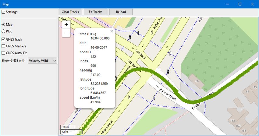
4.12 GNSS Map . . . . . . . . . . . . . . . . . . . . . . . . . . . . . . . . . . . . . 52
4.13 Appearance and Preferences . . . . . . . . . . . . . . . . . . . . . . . . . . . 54
4.13.1 Layout Wizard . . . . . . . . . . . . . . . . . . . . . . . . . . . . . . . 54
4.13.2 Global Preferences . . . . . . . . . . . . . . . . . . . . . . . . . . . . 56
4.13.3 Plot Preferences . . . . . . . . . . . . . . . . . . . . . . . . . . . . . 57
4.13.4 Node Preferences . . . . . . . . . . . . . . . . . . . . . . . . . . . . . 58
4.13.5 Orientation Preferences . . . . . . . . . . . . . . . . . . . . . . . . . 59
4.13.6 Tracker Preferences . . . . . . . . . . . . . . . . . . . . . . . . . . . . 60
4.13.7 FFT Preferences . . . . . . . . . . . . . . . . . . . . . . . . . . . . . . 61
4.14 Updating the Firmware . . . . . . . . . . . . . . . . . . . . . . . . . . . . . . 62
5 The Orientation Algorithm 64
6 Performing an Experiment 65
6.1 Experiment Preparation . . . . . . . . . . . . . . . . . . . . . . . . . . . . . . 65
6.2 Reading and Aligning CSV Log Files . . . . . . . . . . . . . . . . . . . . . . . . 65
7 Troubleshooting 67
7.1 Finding the Serial Port . . . . . . . . . . . . . . . . . . . . . . . . . . . . . . . 67
7.2 Bluetooth Connection . . . . . . . . . . . . . . . . . . . . . . . . . . . . . . . 67
7.3 Slow Signals in Inertia Studio . . . . . . . . . . . . . . . . . . . . . . . . . . . 68
7.3.1 Lowering the Plot Update Speed . . . . . . . . . . . . . . . . . . . . . 68
7.3.2 Reducing the Number of Plots or Nodes . . . . . . . . . . . . . . . . . 68
7.3.3 Enabling Hardware Acceleration and Multi‐threaded Rendering . . . . 68
7.4 Retrieving an Unreachable ProMove‐mini Node . . . . . . . . . . . . . . . . . 68
7.5 Manually Installing the Inertia Driver . . . . . . . . . . . . . . . . . . . . . . . 69
inertia‐technology.com Page 3 of 71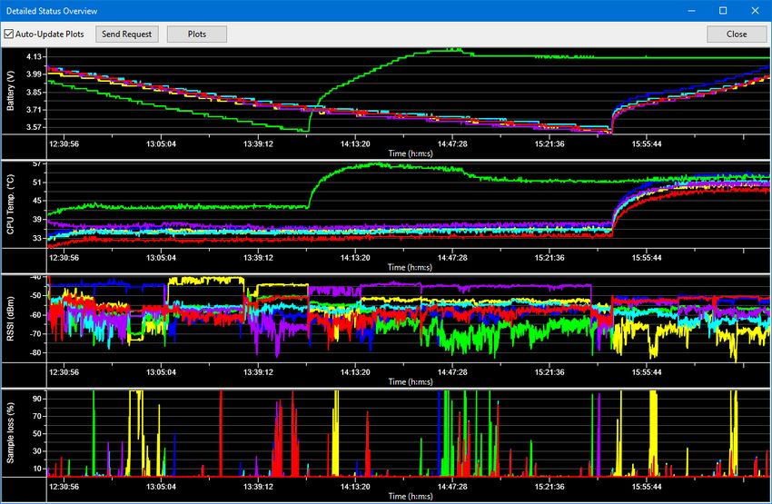
8 Technical Specifications                                                              70
  8.1 Advanced Inertia Gateway Specifications . . . . . . . . . . . . . . . . . . . . . 71

inertia‐technology.com                                                         Page 4 of 71
1      Introduction
The ProMove‐mini is a wireless inertial motion sensor node specifically designed for multi‐
person, multi‐object motion tracking. A network can comprise tens of devices that sample and
transmit motion and orientation information at high data rates in a fully synchronized manner.
The ProMove‐mini features a complete set of 3‐D digital sensors, offering 10 DOF sensor data:
acceleration, turn rate (gyroscope), magnetic field intensity (compass), high‐g acceleration and
barometric pressure. Full 3‐D orientation information, expressed as quaternions, is also made
available to the user.
The sensor data is transmitted wirelessly using the low‐power 2.4 GHz radio to a central node,
the Inertia Gateway, which connects to the computer through USB. Optionally, the sensor data
can be stored on the on‐board flash and retrieved later over USB or wirelessly.
The number of nodes in the network scales with the sampling rates, e.g. a network can have
39 nodes that sample at 200 Hz, or 19 nodes that sample at 500 Hz.
Alternatively, the ProMove‐mini can be equipped with a Dual‐Mode Bluetooth module or a
Bluetooth 4.0 Low Energy module for direct communication to PCs, smartphones and tablets.
The ProMove‐mini is carefully designed for good ergonomics. The curved design makes mount‐
ing and wearing on body parts comfortable, without affecting stability in case of surface mount‐
ing.
Please read the safety instructions in Section 2 carefully. Information about warranty and lia‐
bility can be found at: https://inertia‐technology.com/terms‐and‐conditions/.

                            Figure 1: ProMove‐mini sensor node

inertia‐technology.com                                                              Page 5 of 71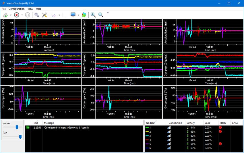
2      Safety Instructions
To avoid a potential safety hazard, please follow the safety instructions below:
    • Do not exceed the maximum input voltage of 5V.
    • Only connect to CE‐certified computers and USB‐adapters.
    • Operate the product at temperatures between 0 and 35°C.
    • Prevent contact with water at all times. Do not charge the product if wet.
    • Once fully charged, remove the product from the charger.
    • Protect the product from violent handling, drops on hard surfaces, excessive shocks or
      mechanical stress.
    • Do not open, crack, pinch or mutilate in any way the product.
    • Do not use the product if it appears damaged or tampered with in any way.
    • Do not attempt to replace the battery, open the enclosure or disassemble the product.
    • Turn off the product before entering an area with potentially explosive atmosphere.
    • Do not overheat the product by exposure to high temperatures or direct sunlight.
    • Do not dispose the product in fire.
    • Do not discard the product in the trash. Follow proper electronic and battery waste
      disposal protocol, as dictated by local authorities.
    • Keep the product out of the reach of children.

inertia‐technology.com                                                             Page 6 of 71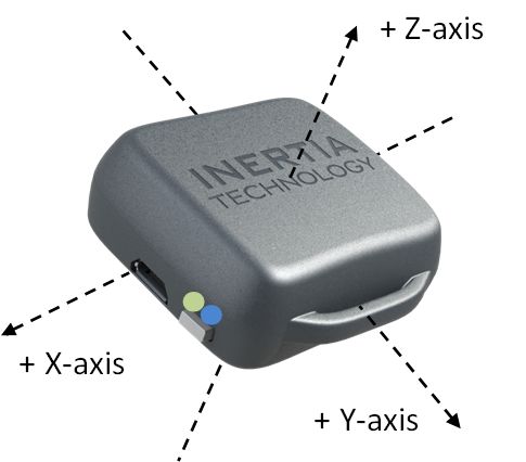
3 Setup
This section describes the high‐level system setup.
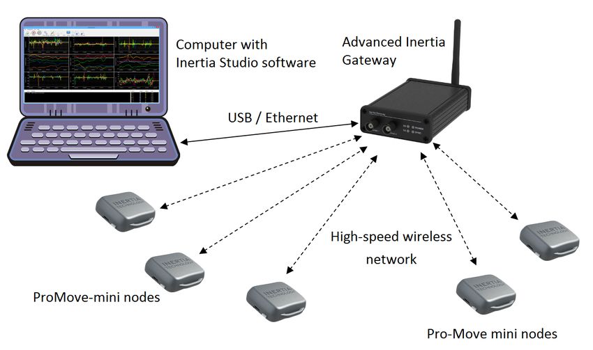
3.1 System Description
The default system consists of a number of ProMove‐mini sensor nodes, the Advanced Inertia
Gateway and Inertia Studio (PC Software) for monitoring and logging the inertial data. The
standard setup is depicted in Figure 2. The sensor nodes communicate wirelessly with the
gateway in the 2.4 GHz ISM band. The gateway is connected through the mini‐USB connector
or the Ethernet connector with a PC that runs Inertia Studio.
Figure 2: Typical system setup
A system could also consist of a single ProMove‐mini node, which can be connected either
through micro‐USB or through Bluetooth to the PC running Inertia Studio.
C++ and Java SDKs are available for developing custom applications that interact with Inertia
devices. The SDKs allow implementations on both desktop and mobile Android platforms.
inertia‐technology.com Page 7 of 71
3.2    Gateway Connections
Figure 3 shows the front and back of the Advanced Inertia Gateway. On the front, the gateway
has two BNC connectors and four blue LEDs with the following functionality:
   • RX: The gateway is receiving data.
   • TX: The gateway is transmitting data.
   • Power: The gateway is powered on.
   • Sync: The gateway is synchronized with an external signal.
The EXT SYNC 1 and EXT SYNC 2 connectors can be configured as Input or Output, with either
Trigger or Sync functionality. See Section 4.10 for more information.
The backside contains a DC power connector, antenna, mini‐USB connector and an 100BASE‐
TX Ethernet connector. The gateway can be connected using the mini‐USB or the Ethernet
connector to the PC.
When using the Ethernet connector, the gateway can be connected directly to the network
adapter of the PC using an Ethernet cable, or to a (wireless) switch/router in the same local
network as the PC. Inertia Studio requires Npcap or WinPcap on Windows and libpcap on Linux
and macOS to access the network adapter and receive the Raw Ethernet data. The gateway
has a local MAC address based on its serial number, e.g. 02:34:56:78:xx:xx, where xx:xx is the
serial number. The gateway sends its data to broadcast address ff:ff:ff:ff:ff:ff using EtherType
protocol 0xbabe.

               Figure 3: The front and back of the Advanced Inertia Gateway

inertia‐technology.com                                                              Page 8 of 71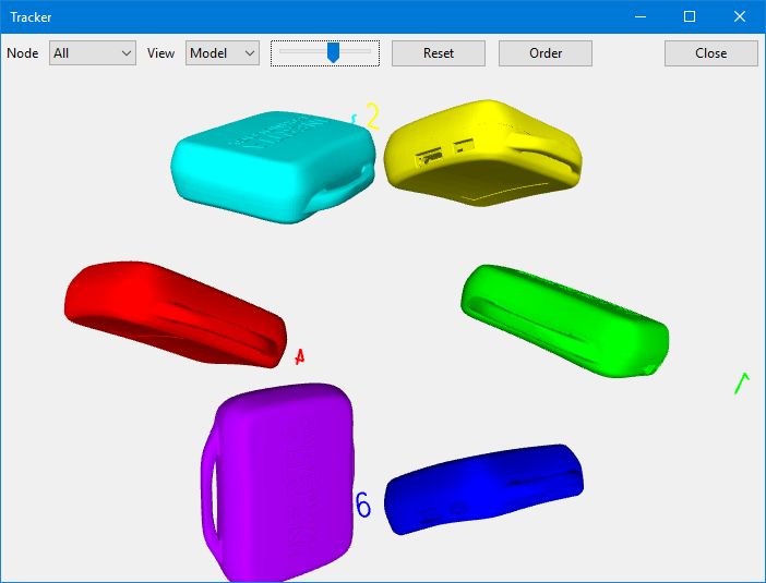
3.3    Node LEDs and Button
Figure 4 shows a ProMove‐mini node and the reference system axes (X, Y and Z) to which the
on‐board sensors are aligned.

            Figure 4: The ProMove‐mini node and the reference X, Y and Z‐axis

The LEDs and the multifunctional button are located next to the micro‐USB connector.
The green LED indicates the node is charging. The blue LED indicates the node is turned on
and sampling data. The blinking rate is determined by the sampling rate. The number of blinks
has the following meaning:
   • Single blink: Not transmitting data.
   • Double blink: Transmitting data via USB or wireless. Synchronized nodes should blink at
     the same time.
   • Five blinks: Logging to flash memory.
The button has the following functionality:
   • Pressing short once: Turns the node on; it is also used to confirm pairing via Bluetooth.
   • Pressing short twice: Starts or stops logging to the flash memory.
   • Pressing long once: Turns the node off. Pressing more than 5 seconds will powercycle
     the node.

3.4    Attachments
Velcro straps can be attached through the handles, as shown in Figure 5.

inertia‐technology.com                                                            Page 9 of 71
Figure 5: A ProMove‐mini with a wristband
3.5 Recharging the Batteries
The internal battery of the ProMove‐mini should be periodically recharged. This can be done
by using a cable connecting the micro‐USB connector of the node to a computer or a standard
USB charger . A fully drained battery takes approximately 1 hour to recharge when turned off,
and 1.5 hours when turned on. During charging, the green LED of the node is on. The gateway
has no internal battery and therefore does not require recharging. Monitoring the battery
voltage can be done using Inertia Studio (see paragraph 4.1.3). The battery is fully charged
around 4.15 V. When the battery is empty (at 3.45 V) the node will turn itself off automatically.
3.6 On‑board Storage
ProMove‐mini nodes are equipped with 2 GB flash memory. Downloading the data from the
flash memory is described in Section 4.4.2.
The flash memory is used to store the following data:
• The sensor node configuration, including the global parameters, the wireless options
and the configuration of the sensors (for information about changing, storing and clear‐
ing the sensor node configuration, see Section 4.8).
• The sensor data, the sampled data of all enabled sensors. More information about stor‐
ing data in the flash memory of a sensor node can be found in Section 4.4. The flash
memory can store a maximum of 510 files.
inertia‐technology.com Page 10 of 714 Inertia Studio
Inertia Studio can be used for realtime visualization of sensor data, logging of sensor measure‐
ments and pre‐computed orientation, and configuration of sensor and wireless parameters.
This section describes Inertia Studio (v3.6.1) in more detail.
Inertia Studio is available for Microsoft Windows 7, Ubuntu 16.04, macOS 10.10 and later ver‐
sions.
4.1 Main Screen
Figure 6 shows the main screen of Inertia Studio, which is divided in the following areas:
• The menu and toolbar at the top (described in Section 4.1.1)
• The sensor data plots in the middle (described in Section 4.1.2)
• The information area at the bottom (described in Section 4.1.3)
In the following, these three areas are presented in detail.
Figure 6: Inertia Studio with six ProMove‐mini nodes, showing data from the accelerometer,
compass and gyroscope
inertia‐technology.com Page 11 of 714.1.1 Toolbar and Menu
The toolbar is used to quickly access the most used functionality of Inertia Studio. This section
describes the default buttons of the toolbar, from left to right (see Figure 7).
Figure 7: Inertia Studio menu and toolbar
• Connect / Disconnect
The Connect / Disconnect button can be used to quickly connect to, or disconnect from an
Inertia device. The drop‐down menu associated with this button opens a list for selecting
the target nodes. See Section 4.2 for more information.
• Record / Stop
When connected to a device, the Record / Stop button can be used to quickly start and
stop logging/recording to file (see Section 4.3). If timed recording is enabled, a small clock
overlay is shown on the icon. The drop‐down menu associated with this button offers rapid
access to the Logging Configuration window (see Section 4.3). The user can also quickly set
the duration of the recording using time‐presets.
• Pause / Resume
The Pause / Resume button is enabled during recording. It can be used to pause and resume
the recording.
• Sensor Settings
The Sensor Settings button opens the Sensor Settings window (see Section 4.8).
• Preferences
The Preferences button opens the Preferences window (see Section 4.13.3).
• Hide / Show
The Hide / Show button toggles between hiding and showing the data in the plots. The
drop‐down menu associated with this button opens a list for selecting the target nodes for
which the data is hidden or shown. An small sign (i.e. red cross or yellow triangle) on the
icon indicates that some data is hidden. This button does not influence the logging.
• Clear (F5)
The Clear button, or F5, clears the plots, legend and node lists. This button does not influ‐
ence the logging.
• Layout
The Layout button opens the Layout Wizard (see Section 4.13.1) and has a drop‐down menu
to switch between layouts.
inertia‐technology.com Page 12 of 71• Tracker The Tracker button opens the Tracker window (see Section 4.11). • Zoom In (F3) / Zoom out (F4) The Zoom buttons, or F3 and F4, can be used to zoom the X‐Axis of all plots in or out. The menu allows access to all the options of Inertia Studio and has the following items: • File —Connect... opens the Connection Configuration window (Section 4.2). —Record opens the Log to File (Section 4.3) and Log to Flash (Section 4.4.1) windows. —Replay... opens the Replay window (Section 4.7). —Download... opens the Download Logfiles window (Section 4.4.2). —Fill‐in Lost Samples... opens the Fill Loss window (Section 4.5). —Export... opens the Export Logfiles window (Section 4.6). —Exit closes Inertia Studio. • Configuration —Sensor Settings... opens the Sensor Settings window (Section 4.8). —I/O Settings... opens the I/O Settings window (Section 4.10). —Sensor Calibration... opens the Calibration Configuration window (Section 4.9). —Preferences... opens the Preferences window (Section 4.13.2). —File Types opens a sub‐menu to configure the supported file types. —Power Down... allows the user to remotely power down specific sensor nodes. • View —Layout Wizard... opens the Layout Wizard (Section 4.13.1). —Tracker opens the Tracker window (Section 4.11). —GNSS Map opens the GNSS Map window (Section 4.12). —Detailed Status opens the Detailed Status window (paragraph 4.1.3). —Toolbox can be used to show or hide the Zoom and Pan sliders, the RTC buttons and the Log and Legend in the information area. —Toolbar can be used to change the appearance of the toolbar. The toolbar can be hidden using the Hide option. The size of the toolbar icons can be modified to Small, Medium and Large. Show Text allows to show or hide the text below the icons. Show I/O Buttons adds two extra buttons to the toolbar for I/O functionality. —Show Data toggles between showing and hiding the incoming data in the plots. —Clear Plots (F5) clears the plots, legend and node lists. —Full Screen (F11) shows Inertia Studio in full‐screen mode. • Help —Check for Updates checks if a new version of Inertia Studio is available, or if new firmware for the connected nodes is available. —Firmware Update... opens the Firmware Update window (Section 4.14). inertia‐technology.com Page 13 of 71
—Software Web Site opens the Inertia Technology software website.
  —Manual (F1) opens the Inertia Studio manual.
  —About shows the current Inertia Studio version and build date.

4.1.2   Plots
Inertia Studio can be configured to display a customizable number of plots that show in real‐
time the sensor data (e.g. accelerometer data), status data (e.g. battery voltage, lost samples)
and processed data (e.g. orientation, Norm, FFT). The shown plots and layout can be cus‐
tomized via the Layout Wizard (see Section 4.13.1). The X‐axis of the time‐plots represent the
number of seconds since the gateway was started.
The mouse can be used to zoom and pan the plot. Holding the left mouse button while moving
the mouse creates a zoom‐box. Releasing the left mouse button zooms to the selected data.
Not that Auto‐scaling resets the Y‐axis zoom. A plot can be panned by holding the right mouse
button and moving the mouse. By default, the X‐axis is automatically set to the latest received
data. Disable Show Data or use the pan slider (see Section 4.1.3) to prevent this.
Right‐clicking on a plot provides the following options (see Figure 8):

                            Figure 8: Plot right‐click pop‐up menu

   • Fit: Fits all received data in the plot.
   • Zoom in/out: Zooms the plot in or out. The Zoom buttons in the toolbar and the Auto‐
     scaling option (see Section 4.13.3) can be used to reset the zoom.
   • Lock X‐axis...: Locks the X‐axis to a specified range by showing a pop‐up window in which
     the minimum and/or maximum values of the X‐axis can be set. When the axis is locked,
     a ← and/or → symbol is shown at the bottom right and/or left corner of the plot. This
     option is only enabled for FFT plots.
   • Lock Y‐axis...: Locks the Y‐axis to a specified range by showing a pop‐up window in which
     the minimum and/or maximum values of the Y‐axis can be set. When the axis is locked,
     a ↑ and/or ↓ symbol is shown at the left top and/or bottom corner of the plot. Locked
     plots do not auto‐scale.
   • Auto‐Scale Y‐axis: Toggle automatically scaling the Y‐axis. This overrules the global auto‐
     scaling option in Section 4.13.3.

inertia‐technology.com                                                             Page 14 of 71
• Save as SVG...: Save the plot as a SVG image. 4.1.3 Information Area The information area at the bottom of the main screen shows the list of event messages and the legend with connected nodes. In addition, a zoom‐slider, a pan‐slider and buttons to set and get the time of the nodes can be added to the information area via the menu (View, Toolbox). Notification Area Event notifications are displayed in the notification area. They give information about the out‐ come of certain actions, such as plugged‐in or removed devices, connecting to or disconnecting from a device, starting or stopping logging, downloading or exporting files, modifying sensor configurations, etc. By clicking the header of the time column, the notifications can be sorted in ascending or descending time order. Right clicking an item in the list provides the following options: copy the selected line(s), copy all lines, and clear the notification area. The icon in front of a message indicates the notification type. A green check‐mark means success, a red cross means error, an orange triangle means warning and a blue circle means information. Legend The legend contains a list of all the nodes of which sample data is received. The first column shows the selected port, the line colour and node ID for each node. The node ID can be ex‐ tended with a name in Section 4.13.4. The second column (Signal) displays the radio signal strength (when connected via a gateway), or the transmission type (in case the node is con‐ nected via USB or Bluetooth). The third column (Battery) shows the battery level for each node, and whether the node is charging. The fourth column (Loss) shows the percentage of lost sam‐ ples over the last period (see also Section 4.13.2). The fifth column (Flash) shows whether the node is logging to flash or not. The sixth column (GNSS) shows whether a node equipped with a GPS or GNSS sensor has a fix or not. The legend can be sorted on every column. Columns can be hidden by right‐clicking the column header. Double‐clicking on the legend opens the Detailed Status window (see paragraph 4.1.3). The radio strength is updated every second. The battery level is, by default, updated every ten seconds. The loss update interval can be configured via the global preferences (see Sec‐ tion 4.13.2). Zoom, Pan and RTC The zoom and pan sliders can be used to change the visible data in the plots. The zoom slider behaves the same as the zoom buttons in the toolbar (Section 4.1.1) and allow to zoom the X‐axis in or out. The pan slider allows the move back in time and show older data. The max‐ imum number of seconds to pan can be configured in the global settings (Plot History in Sec‐ tion 4.13.2). If panning is active, plots are not updated with new sample data. inertia‐technology.com Page 15 of 71
The RTC buttons can be used the set and get the time of the Real‐Time Clock of a node. The
RTC is also set automatically when a node is discovered by Inertia Studio. When setting the
time, the current UTC time of the PC is send to the nodes.

Detailed Status
The Detailed Status Overview window (see Figure 9) can be accessed by double clicking an item
in the legend or via the View menu, sub‐menu Detailed Status. The window shows detailed
information about the battery level, CPU temperature, external input, RSSI and sample loss of
the connected nodes. The plots are cleared when (re)connecting to a device.

                            Figure 9: Detailed Status information

The battery, temperature and external input plots are updated when status information from
a node is received via automatic status messages (usually every ten seconds). The RSSI plot
is updated every second with the average value of the received RSSI information. The sample
loss plot is updated every second with the detected sample loss. The time on the X‐axis is the
system time. A battery is fully charged when the voltage is around 4.15 V. The node powers
down when the voltage drops below 3.45 V.
A checkbox is available to disable automatic updating of the plots. This can be used to prevent
the plots from resetting when zoomed in. The Send Request button broadcasts a message to
all nodes with a request to send the current battery and CPU temperature value. The Plots
button can be used to show or hide specific plots.

inertia‐technology.com                                                            Page 16 of 71
4.2 Connecting to a Device
In this section we describe how an Inertia device can be connected to the PC, using the follow‐
ing connections:
• USB: Any Inertia device can be connected to the PC using USB. The micro‐USB connector
of the ProMove‐mini and the mini‐USB connector of the gateway can be used for direct
connection to the PC using a USB cable.
• Bluetooth: A ProMove‐mini node with Bluetooth can be connected wirelessly using
Bluetooth to the PC. See Section 7.2 on how to pair with a Bluetooth device.
• Ethernet: The Advanced Inertia Gateway can also be connected using Ethernet to the
PC. The gateway can be connected either directly to the network adapter of the PC using
an Ethenet cable, or indirectly using an Ethernet cable to a (wireless) switch or router
that is in the same local network as the PC. Inertia Studio requires Npcap or WinPcap on
Windows and libpcap on Linux and macOS to access the network adapter and receive
the Raw Ethernet data.
The connection can be started via the Connect button in the toolbar or from the File menu
item, option Connect....
4.2.1 Connecting to a Device Using the Toolbar
Pressing the arrow next to the Connect button in the toolbar opens the drop‐down menu
shown in Figure 10:
• The option Connect... opens the Connection Configuration window, which is explained
in Section 4.2.2.
• The option Available... opens a pop‐up window with all the available devices, including
the active network adapters. A setting in the Global Preferences (Section 4.8.1) can hide
the network adapters from the list of available devices.
• Below the line, a list is shown with the names of the available Inertia devices connected
through USB or Bluetooth and the active network adapters, i.e. the local and/or the
wireless network adapters. Next to them, the corresponding port numbers are given. A
• symbol in front of the name indicates the device is selected. A ► symbol in front of
the name indicates the device is connected.
Select the desired device and press the Connect button in the toolbar to connect.
4.2.2 Connecting to a Device Using the Menu
The option Connect... from the File menu item opens the Connection Configuration window
from Figure 11. The window shows a list with Stored Configurations, i.e. all the connections
to Inertia devices that were previously used and those that are currently available. The list
inertia‐technology.com Page 17 of 71Figure 10: Connect drop‐down menu
includes the devices connected through USB or Bluetooth and the active network connections,
e.g. the local and/or the wireless network connections. The port name (“com*“ on Windows
and “/dev/*“ on Linux) is shown next to the device name. A green dot indicates the device is
available. The ► symbol indicates the device is connected.
By pressing the Available? button, the list is updated and a pop‐up window with all the avail‐
able devices is shown. The Show button loads the selected connection into the main screen.
The Add... button can be used to manually add a device to the list if it is not automatically de‐
tected. The Remove button removes a selected device from the list. The Connect/Disconnect
button starts and shows, or stops, the selected connection with the device.
Figure 11: Connection Configuration
inertia‐technology.com Page 18 of 714.3 Logging to File
When connected to an Inertia device, the incoming data can be stored/recorded in a log file.
The default file format is itlog (Inertia Log File). Incoming samples, node information and con‐
figurations, etc, are stored in the file. An itlog file can be exported to a different format (see
Section 4.6). The itlog format also supports filling in lost samples after an experiment is fin‐
ished, see Section 4.5.
There are two options that can be used to enable logging to file:
1. By using the Record button from the toolbar; to change the settings for creating a log
file, select the Log to File... option from the drop‐down menu of the Record button; this
option opens the Logging Configuration window for logging to file (see Figure 12).
2. By selecting the Log to File... option from the File menu, Record item; this option opens
the same Logging Configuration window for logging to file (see Figure 12).
Figure 12: Log to File Configuration
In the Logging Configuration window, the settings for creating a log file can be modified as
follows:
• Filename: The name of the log file. The default file format is itlog.
inertia‐technology.com Page 19 of 71• Description: A description that can be added to the beginning of the (exported) log file.
• Compression: An optional compression format used for the log file, resulting in a smaller
file size. Supported compression methods are: gzip (.gz, GNU Zipped Archive), bzip (.bz2,
BZIP2 Compressed Archive) and zlib (.Z, UNIX Compressed Archive).
• Unique Filename: Selects the way of handling existing log files with the same name:
– Overwrite: The existing file is overwritten.
– Append to File: The data is added to the existing file.
– Auto‐Number: Files are numbered in sequence with the following naming convention:
[_№].ext, where ext is the file extension and № is the sequence number;
this number is automatically increased every time a log file with the same name is
created.
– Date in Filename: The current date and time are added to the filename; the timestamp
is formatted as described in ISO 8601 (i.e. [YYYYMMDDThhmmss_].ext).
• Stop Logging After: This option can be enabled to automatically stop logging to file. The
duration can be entered as hh:mm:ss. When active, a countdown is shown in the toolbar.
• Start Flash Logging: Starts (and stops) logging to flash when a log file is created. This option
is enabled by default when Fill‐in Lost Samples is enabled.
• New File Every: Start logging to a new file once the provided number of seconds or file size
is reached. Fill‐in Lost Samples and Export should be disabled.
• Fill‐in Lost Samples: Fills‐in lost samples when logging to file is finished (see Section 4.5).
• Export: Exports the log file when logging to file (including filling in lost samples) is finished.
The button opens the Section 4.6 window.
If a device is connected, the Record button can be used to save the settings and start creating a
log file. If the device is disconnected, the Save button can be used to save the current settings.
The Stop button can be used to stop logging. During logging, the Pause and Resume buttons
can be used to pause, respectively resume, logging to file. These buttons behave similarly to
the buttons in the toolbar (i.e. Record / Stop and Pause / Resume), described in Section 4.1.1.
inertia‐technology.com Page 20 of 714.4 Logging to Flash
ProMove‐mini nodes have an internal flash memory that can be used to store sensor data.
Flash logs are used to fill in lost samples after an experiment, as described in Section 4.5. Flash
logs can also be created manually, as described in Section 4.4.1. Section 4.4.2 describes the
way the flash logs can be downloaded to the PC.
4.4.1 Starting and Stopping a Flash Log
The Log to Flash option from the File menu, Record item, opens the Logging Configuration
window for logging to flash (see Figure 13).
The Logging Configuration window shows the list of all devices in the network. For each node
in the list, the ► symbol indicates whether the node is logging to flash or not. If a timer is used
when starting the flash log (the Stop Logging After option is enabled), a countdown is visible
in the list. The last column in the list shows the sensor data types that are logged to flash (see
Section 4.8 to enable or disable sensors).
Figure 13: Log to Flash Configuration
The Start / Stop buttons can be used to send a command to the checked node(s) to start or stop
logging to flash. The Stop Logging After option activates a timer for stopping the flash logging.
Closing Inertia Studio while a timer is active does not determine a node to stop logging to flash.
inertia‐technology.com Page 21 of 71The format of the timer is hh:mm:ss. During logging to flash, the blue led blinks in short bursts.
Starting or stopping a flash log can also be done by pressing shortly twice on the button of the
ProMove‐mini (see Section 3.3).
When starting or stopping a flash log, a notification message appears in the information area at
the bottom of the main screen with the response from the node, indicating success or failure.
A failure can occur when logging to flash is already started (or stopped) or when the maximum
number of 510 files is reached.
Flash logs are named LOG.LOG, where № is the first available number starting from 1.
The creation date of the flash log is also recorded. The date is based on the internal clock
of the node. If the battery of a node is fully drained, the clock is reset, which can result in
an incorrect creation date. The internal clock is automatically synchronized with the PC time
when data from a node is received by Inertia Studio.
A ProMove‐mini sampling at 200 Hz with all sensors enabled uses about 20 MB of flash per
hour.
4.4.2 Downloading a Flash Log
To download flash logs, the node should be directly connected via an USB cable to the PC.
Downloading over radio/Bluetooth is supported, but is generally much slower and could fail
due to packet‐loss. By selecting the Download... option from the File menu, the Download
Flash Logs window appears, as shown in Figure 14. When a node is selected in the drop‐down
list, status information about the internal flash is shown, and the File list is updated with the
flash logs present on the internal flash of the node. The filename, file‐size and creation date
(local time) of each file is shown in the list. Selecting a node or using the Refresh button on the
right hand side will update the status information and file‐list. Active files (e.g. files currently
being created) are not included in the file list.
To download a file, select it in the File list and adjust the following options:
• Destination: The name of the file (itlog format). Several wildcards are supported in the
filename:
– {name} or %s: Insert the full flash file name (without extension).
– {no} or %d: Insert the number of the flash file (e.g. 34 for LOG34.LOG).
– {date} or %c: Insert the creation date of the flash file (in ISO 8601 format).
– {id} or %i: Insert the node ID.
• Unique Filename: Selects the way of handling existing log files with the same name (same
as in Section 4.3).
• Use Date from Flash File: Set the creation date of the file to the date of the flash file.
inertia‐technology.com Page 22 of 71• Export: Export the file when downloading is finished. Use the button to open the Export
Settings. (see Section 4.6).
Press Download to start the download. If the node is transmitting data, transmission will be
temporarily disabled until the download is finished.
During downloading, the progress is shown in the list. Information about the progress is also
shown in the information area at the bottom of the main screen (see paragraph 4.1.3). When
downloading is in progress, the Cancel button can be used to cancel the process. If a file is
being downloaded, other files of the node can be queued so they will start downloading as
soon as the current file is finished. Select one or more files, adjust the file options, an press
Queue.
Figure 14: Download Flash Logs
4.4.3 Deleting Flash Logs
Flash logs can be removed from the flash memory using the Format button in the Download
Logfiles window (Figure 14). This action removes all files from the internal flash memory. For‐
matting takes about 5 to 10 seconds. A message is shown when formatting is finished.
Do not turn the nodes off during formatting!
inertia‐technology.com Page 23 of 714.5 Filling in Lost Samples
When performing an experiment with wireless sensor nodes, there is almost always some data
loss. This loss can be filled in automatically after the experiment is finished. This feature is
available only for experiments performed with a gateway, when the sensor nodes are in Syn‐
chronous mode (see Section 4.8.1 for details about sampling mode). If the sensor nodes are in
Stand alone mode, or if the sensor nodes are connected using a USB cable or using Bluetooth,
this feature is not available.
The sections below explain this process of filling in the lost samples.
4.5.1 Automatic
Enable Fill‐in Lost Samples when creating a logfile (see Section 4.3). Once logging is stopped,
a pop‐up is shown informing that missing data will be filled in. Once continued, the Fill‐in Lost
Samples window is shown (Figure 15) and missing data is automatically filled in.
The process consists of three stages:
1. First, the existing logfile is analyzed and missing data of each node is identified. During
this stage, a progress bar for each node is filled with blue bars. The tint of the color rep‐
resents the amount of lost data: white is 100% loss, dark blue is 0% loss. The percentage
inside the progress bar is the total percentage of samples available.
2. During the second stage, the missing data is requested wirelessly from the nodes (Fig‐
ure 15). The progress bars are actively being updated to reflect the received data. The
lighter segments change to dark‐blue.
3. In the third stage, the received data is merged into the itlog file (Figure 16). The progress
bars are filled with green bars to show the progress. If there is still some missing data,
sections in a progress bar are made red and messages with information about the miss‐
ing sections are added to the notification area. A manual restart could fill in the remain‐
ing missing samples (see Section 4.5.2).
Figure 15: Requesting Figure 16: Merging
Once the process is finished, and if Export was enabled when the logfile was created, the file
inertia‐technology.com Page 24 of 71is exported in the background. If the fill‐loss process is canceled using the Cancel button, a
pop‐up asking to continue with export is shown.
The Fill‐in speed during the second stage is dependent on the configured number of nodes in
the network (Section 4.8.1). The value should be close to the actual number of nodes, e.g. 6
or 9 (default) when using 6 nodes.
4.5.2 Manual
Filling in lost samples can also be started manually. Open the window via the menu (File, Fill‐in
Lost Samples...) and expand the manual settings using the Manual Settings arrow (Figure 17).
Provide the following parameters:
• File: One or more itlog files to be filled in.
• Port: The port used to access the node(s), usually the port of the gateway.
• Export: Export the itlog file when filling in lost samples is finished or canceled. Use the
button to open the Export Settings. (see Section 4.6).
• Backup: Keep a backup of the unfilled file (named _BACKUP_.itlog).
• Slots: Temporarily change the number of slots (to a lower value) to increase the fill‐loss
speed. This should be equal or higher than the number of devices in the network. Leave
empty or use 0 for the default number of slots.
Use Start to start the process.
Figure 17: Manual settings
4.5.3 Details
The Details arrow can be used to expand the window and show a list with all the status mes‐
sages that have appeared. The items in the list can be copied or cleared using the Copy and
inertia‐technology.com Page 25 of 71Clear buttons. The Auto‐scroll checkbox can be used to enable or disable automatic scrolling of the list to the latest message. inertia‐technology.com Page 26 of 71
4.6    Exporting a Logfile
Inertia Log Files of type itlog can be exported to different file types using the Export Logfiles
window (see Figure 18), which can be accessed from the menu (File, Export). The following
parameters can be modified:
• Source: The itlog file(s) to export. The Destination filename is automatically updated to
  match the source name and the selected file format.
• Format: The file format to export the itlog file to. Settings specific to the file format can be
  modified via the Configure button.
• Compression: An optional compression format used for the exported file, resulting in a
  smaller file size. Supported compression methods are: gzip (.gz, GNU Zipped Archive), bzip
  (.bz2, BZIP2 Compressed Archive) and zlib (.Z, UNIX Compressed Archive).
• Unique Filename: Selects the way of handling existing log files with the same name (same
  as in Section 4.3).
Use the Start button to save the settings and export the file(s). Active and previously exported
files are shown in the Activity List. Double‐clicking an item opens the exported file in its default
program. An active item can be canceled using the Cancel button. previously exported files
in the activity list can be cleared using the Clear button. The folder of a selected item can be
opened using the Open Folder button.

                                    Figure 18: Export Logfiles

inertia‐technology.com                                                                Page 27 of 71
4.6.1 CSV Settings
Inertia Log Files can be exported to a Comma Separated Values file (CSV). The CSV Settings can
be modified in the CSV Settings window (see Figure 19), accessible via the menu (Configuration,
File Types, CSV Settings...) or from the Export window.
A CSV file starts with a header identifying each column. Each subsequent line in the CSV file
consists of a timestamp and the sensor data sampled at that timestamp.
The following settings can be modified for the CSV file format:
• One File per Node: A separate file is created for each node; the node number is appended
to the filename: [_node№].ext. When disabled, one file with data from all nodes
is created.
• Repeat Previous Value: When sensors have a lower sampling rate than the global sampling
rate, empty values are added to the CSV file (no value between commas). For example,
when the global rate is 200 Hz, the compass samples at 100 Hz, resulting in empty values
every other line. By using this option, instead of logging an empty value, the last received
value is repeated until a new value is received.
• Add Info to Beginning of File: Add information such as node information, sensor settings,
units of measurement, a description, etc, to the beginning of the log file. The information
lines start with a #.
The sensor data added to the CSV file can be configured by (un)checking the desired Columns.
Default columns for ProMove‐mini, V‐Mon 4000 and All can be loaded using the Defaults but‐
tons. Apply will save the settings and close the window, Close will discard any modified settings
and close the window.
Figure 19: CSV Settings
inertia‐technology.com Page 28 of 714.6.2 MAT Settings
Inertia Log Files can be exported to a MatLab MAT file. The MAT Settings can be modified in
the MAT Settings window (see Figure 20), accessible via the menu (Configuration, File Types,
MAT Settings...) or from the Export window.
The MAT file contains a global structure array with a field for each node structure. Each node
structure contains four fields. Field columns contains the column names and indices of the
columns, fields combines multiple columns into one field (e.g. ax, ay and ax into accelero‐
meter), data contains the sensor data, and samplingRate contains the sampling rate.
The following settings can be modified for the MAT file format:
• Struct Name: The name of the global structure array.
• MAT Version: The MAT‐file version (see MatLab documentation).
• MAT Compression: Enable compression of the MAT file.
• No. of Samples: The number of samples in the MAT file. This option is not relevant when
exporting an itlog file to MAT. Only when logging directly to a MAT file, the number of sam‐
ples to store needs to be known beforehand. If more (or less) samples are logged, these are
ignored (or filled with NaN).
The sensor data added to the MAT file can be configured by (un)checking the desired Columns.
Default columns for ProMove‐mini, V‐Mon 4000 and All can be loaded using the Defaults but‐
tons. Apply will save the settings and close the window, Close will discard any modified settings
and close the window.
Figure 20: MAT Settings
inertia‐technology.com Page 29 of 714.6.3 Visual3D Settings
Inertia Log Files can be exported to a Visual3D ascii file. The Visual3D Settings can be modified
in the Visual3D Settings window (see Figure 21), accessible via the menu (Configuration, File
Types, Visual3D Settings...) or from the Export window.
The Visual3D ascii file starts with a header identifying each column. Each subsequent line in
the file represents a frame at a specific time point with data from all sensor nodes.
The following settings can be modified for the Visual3D file format:
• Repeat Previous Value: When a sensor value is missing, use the previous value when avail‐
able or use the Empty Value.
• Empty Value: Use this value when there is no known sensor value.
• Owner: The source of the data.
• Point Rate: Add a point rate time signal and set the start time.
• Analog Rate: Add an analog rate time signal and set the start time.
When data of individual sensor nodes is in separate files, for example when downloaded from
flash, it can be merged together before exporting to a Visual3D ascii file. Enable Merge Before
Converting and provide an optional name to use for the merged file. Select all the files to
merge in the Export window.
The sensor data added to the Visual3D file can be configured by (un)checking the desired
Columns. Default columns for ProMove‐mini, V‐Mon 4000 and All can be loaded using the
Defaults buttons. Apply will save the settings and close the window, Close will discard any
modified settings and close the window.
Figure 21: Visual3D Settings
inertia‐technology.com Page 30 of 714.7 Replaying a Logfile
The Replay Logfile window can be used to replay a previously created logfile in real‐time, or
analyze and plot an entire logfile.
Figure 22: Replay Logfile Figure 23: Analyze Logfile
4.7.1 Real‑Time
Real‐time replay has the following options:
• Logfile: The logfile that will be replayed.
• Hardware Type: (CSV only) The hardware type of the device used in the logfile. This is
necessary to determine to correct initial orientation in the tracker.
• Rewrite Replay: (CSV only) The logfile will be rewritten to a new file (same name, with ‐
replay appended), and the orientation (Euler angles and/or quaternions) will be (re)calculated.
• Sampling Rate: The sampling rate used in the logfile. Used to calculate the Read Interval.
• Number of Nodes: The number of nodes in the logfile. This is used to calculate the Read
Interval.
• Read Interval: The number of samples to read per second. The initial value is deter‐
mined by the Sampling Rate and Number of Nodes, but the interval can be manually
adjusted. During a replay, the slider can be used the change the speed of the replay.
A replay is started with the Start button, and stopped with the Stop button. During the replay,
it can be paused with the Pause button. The buttons in the toolbar can also be used to control
inertia‐technology.com Page 31 of 71the replay. Replays are added to the drop‐down menu of the Connect button. Finished replays
are removed from the drop‐down menu when the Available... option is used.
4.7.2 Analysis
Replay analysis can be used to analyze a logfile and detect timestamp issues. It detects Roll‐
backs (timestamp is lower than the previous timestamp), for example when the sampling rate
is changed during the experiment. Duplicate Timestamps are detected when subsequent time‐
stamp are the same. And Gaps, when samples are lost.
It has the following options:
• Logfile: The logfile that will be analyzed.
• Rollbacks: Detect and show timestamp rollbacks in the log.
• Duplicate Timestamps: Detect and show duplicate timstamps in the log.
• Gaps: Detect and show timestamp gaps in the log.
• Show Sample Data in Plots: Collect all the sample data and show them in the plots once
analysis is finished. For large logfiles, this requires a lot of memory.
Analysis is started with the Start button, and stopped with the Stop button. During the analysis,
it can be paused with the Pause button. Once the analysis is finished the data of the logfile is
shown in the plots. When the plot layout is changed, Reload Plot can be used to recreate the
plots. Clear Results will clear the log and remove the collectd sample data from memory.
inertia‐technology.com Page 32 of 714.8 Configuring the Sensors
The Sensor Settings window can be used to modify the configuration of Inertia nodes. This
window is accessible via the toolbar and via the Configuration menu, item Sensor Settings....
Once a device is connected, the configuration options of the detected Inertia nodes is shown
in this window.
Figure 24: Sensor Settings
Figure 24 shows the Sensor Settings window, which is divided in the following areas:
• The node list area, marked with green in Figure 24, contains the list of devices available
via the currently selected connection. When a node is selected, its configuration options
are shown in the sensor tree. When a node is checked by using the checkbox beside it,
the actions of the buttons refer to this node. In Figure 24, all nodes are checked, so the
configuration is applied to all these nodes after pressing the Apply Settings button.
• The sensor tree, marked with red in Figure 24, shows the available configuration op‐
tions of the selected nodes in the node list. When choosing an option in the tree, the
corresponding configuration settings are shown in the settings panel. The different con‐
figuration options in the sensor tree are discussed in the subsequent sections.
• The buttons, marked with blue in Figure 24, have the following functions:
inertia‐technology.com Page 33 of 71– Refresh This button can be used to request all the configurations from all nodes.
The purpose is to make sure that configurations are successfully applied and cor‐
rectly retrieved by Inertia Studio.
– Store This button stores the current configuration of the checked nodes in their
flash memory, so the settings are retained when the nodes are turned off. The
button is not visible if configurations are automatically stored (Section 4.13.2).
– Restore This button can be used to restore all the configurations of the checked
nodes. The nodes are reset to their factory‐default settings.
– Apply Settings This button applies all the modified settings (shown bold in the sen‐
sor tree) to the checked nodes in the list. If no settings are modified, the currently
shown settings are applied If settings are stored automatically, a 15 second count‐
down is shown.
– Close This button closes the window, discarding all modified settings.
• The settings panel, marked with yellow in Figure 24, shows the settings available for
the selected configuration option of the selected node in the node list. These settings
are discussed in detail in the subsequent sections. When invalid or not recommended
settings are used, these settings are marked with a red (invalid) or orange (not recom‐
mended) colour. Invalid settings cannot be applied. Error, warning and information
messages are shown below the Apply Settings and Close buttons. The settings panel
also contains a Refresh and Restore button at the top‐left corner. These buttons can be
used to refresh or restore the selected configuration of the selected node.
4.8.1 Global Settings
By selecting the Global configuration option from the sensor tree, the global settings can be
edited, as shown in Figure 25:
• Transmit Data: Data transmission can be switched off by unchecking the check‐box. Nodes
keep sampling (i.e. to store data in the flash memory).
• Sampling Rate (Hz): Selects the sampling rate used by the sensors. Some sensors may be
limited to a lower sampling rate. When using Synchronous sampling mode, the default max‐
imum number of nodes supported by the network for a selected sampling rate is shown on
the right. The maximum sampling rate is 1000 Hz.
• No. of Nodes: The number of nodes in the network to which the device is currently con‐
figured. For gateways this can be modified to match the configuration of the node(s). For
nodes this is automatically changed to match the gateway settings. The combination of
Sampling Rate and No. of Nodes determine the number of samples in a radio packet. For
best performance, this should be a round number.
inertia‐technology.com Page 34 of 71• Sampling Mode: Inertia nodes can be configured to Synchronous or Stand‐alone sampling.
When sampling synchronously, the gateway dictates the time when the nodes take a sample.
Nodes will not take samples until a gateway is detected. In stand‐alone mode, each node
decides on its own when to take a sample.
• Transmit Type: Data can be transmitted using Wireless (Radio or Bluetooth), USB or both.
• Frequency Channel: Selects the frequency channel used by the Radio. To establish a con‐
nection, the channel of the nodes has to be the same as the channel of the gateway. When
changing channel, it is recommended to first change the frequency channel of the nodes,
and then the channel of the gateway.
• Disable Radio: Disable to radio, for example to save power. The device will not be accessible
anymore, except via USB.
Figure 25: Global Settings
inertia‐technology.com Page 35 of 714.8.2 Accelerometer Settings
By selecting the Accelerometer configuration option from the sensor tree, the accelerometer
settings can be edited, as shown in Figure 26:
• Enabled: Enables sampling of the accelerometer.
• Transmit Data: If the accelerometer is enabled, data will be transmitted. this is overruled
by global transmission settings (see Section 4.8.1).
• Log to Flash: If the accelerometer is enabled, data will be logged to flash. See Section 4.4.1
to start a flash log.
• Sampling Rate (Hz): The sampling rate of the accelerometer (maximum 1000 Hz).
• Range (g): Sets the maximum acceleration that can be measured. Supported options are:
±2, 4, 8 and 16 g. A lower range has a higher sensitivity.
• Calibration: Advanced option that adjusts the scaling and offset of each axis (see Section 4.9
for details about the calibration method).
Figure 26: Accelerometer Settings
inertia‐technology.com Page 36 of 714.8.3 Compass Settings
By selecting the Compass configuration option from the sensor tree, the compass settings can
be edited, as shown in Figure 27:
• Enabled: Enables sampling of the compass.
• Transmit Data: If the compass is enabled, data will be transmitted. this is overruled by global
transmission settings (see Section 4.8.1).
• Log to Flash: If the compass is enabled, data will be logged to flash. See Section 4.4.1 to
start a flash log.
• Sampling Rate (Hz): The sampling rate of the compass (maximum 100 Hz).
• Range (gauss): Shows the maximum magnetic induction that the compass can measure,
which is ±49 gauss.
• Calibration: Advanced option that adjusts the scaling and offset of each axis (see Section 4.9
for details about the calibration method).
Figure 27: Compass Settings
inertia‐technology.com Page 37 of 714.8.4 Gyroscope Settings
By selecting the Gyroscope configuration option from the sensor tree, the gyroscope settings
can be edited, as shown in Figure 28:
• Enabled: Enables sampling of the gyroscope.
• Transmit Data: If the gyroscope is enabled, data will be transmitted. this is overruled by
global transmission settings (see Section 4.8.1).
• Log to Flash: If the gyroscope is enabled, data will be logged to flash. See Section 4.4.1 to
start a flash log.
• Sampling Rate (Hz): The sampling rate of the gyroscope (maximum 1000 Hz).
• Range (°/s): Sets the maximum rotational velocity the gyroscope can measure. Supported
options are: ±250, 500, 1000 and 2000 °/s. A lower range has a higher sensitivity.
• Offset Correction: The gyroscope has a factory, temperature dependent, offset. Enable an
algorithm that zeros the gyroscope axes when no movement is detected.
• Calibration: Advanced option that adjusts the scaling and offset of each axis.
Figure 28: Gyroscope Settings
inertia‐technology.com Page 38 of 714.8.5 Barometer Settings
By selecting the Barometer configuration option from the sensor tree, the barometer settings
can be edited, as shown in Figure 29:
• Enabled: Enables sampling of the barometer.
• Transmit Data: If the barometer is enabled, data will be transmitted. this is overruled by
global transmission settings (see Section 4.8.1).
• Log to Flash: If the barometer is enabled, data will be logged to flash. See Section 4.4.1 to
start a flash log.
• Sampling Rate (Hz): The sampling rate of the barometer (maximum 25 Hz).
• Range (hPa): Sets the pressure range the barometer can measure, which is 260‐1260 hPa.
• Calibration: Advanced option that adjusts the scaling and offset.
Figure 29: Barometer Settings
inertia‐technology.com Page 39 of 714.8.6 High‑G Accelerometer Settings
By selecting the Acclerometer (High G) configuration option from the sensor tree, the high‐g
accelerometer settings can be edited, as shown in Figure 30:
• Enabled: Enables sampling of the high‐g accelerometer.
• Transmit Data: If the high‐g accelerometer is enabled, data will be transmitted. this is over‐
ruled by global transmission settings (see Section 4.8.1).
• Log to Flash: If the high‐g accelerometer is enabled, data will be logged to flash. See Sec‐
tion 4.4.1 to start a flash log.
• Sampling Rate (Hz): The sampling rate of the high‐g accelerometer (maximum 1000 Hz).
• Range (g): Sets the maximum acceleration the high‐g accelerometer can measure. Sup‐
ported options are: ±100, 200 and 400 g. A lower range has a higher sensitivity.
• Calibration: Advanced option that adjusts the scaling and offset of each axis.
Figure 30: High‐G Accelerometer Settings
inertia‐technology.com Page 40 of 71You can also read