RADIv1: a non-steady-state early diagenetic model for ocean sediments in Julia and MATLAB/GNU Octave
←
→
Page content transcription
If your browser does not render page correctly, please read the page content below
Geosci. Model Dev., 15, 2105–2131, 2022
https://doi.org/10.5194/gmd-15-2105-2022
© Author(s) 2022. This work is distributed under
the Creative Commons Attribution 4.0 License.

RADIv1: a non-steady-state early diagenetic model for ocean
sediments in Julia and MATLAB/GNU Octave
Olivier Sulpis1,2 , Matthew P. Humphreys3 , Monica M. Wilhelmus4,5 , Dustin Carroll5,6 , William M. Berelson7 ,
Dimitris Menemenlis5 , Jack J. Middelburg1 , and Jess F. Adkins8
1 Department   of Earth Sciences, Utrecht University, Utrecht, the Netherlands
2 Department   of Earth and Planetary Sciences, McGill University, Montreal, Canada
3 Department of Ocean Systems (OCS), NIOZ Royal Netherlands Institute for Sea Research, Texel, the Netherlands
4 Center for Fluid Mechanics, School of Engineering, Brown University, Providence, USA
5 Jet Propulsion Laboratory, California Institute of Technology, Pasadena, USA
6 Moss Landing Marine Laboratories, San José State University, Moss Landing, USA
7 Department of Earth Sciences, University of Southern California, Los Angeles, USA
8 Geological and Planetary Sciences, California Institute of Technology, Pasadena, USA

Correspondence: Olivier Sulpis (o.j.t.sulpis@uu.nl)

Received: 22 June 2021 – Discussion started: 5 August 2021
Revised: 28 January 2022 – Accepted: 3 February 2022 – Published: 11 March 2022

Abstract. We introduce a time-dependent, one-dimensional         tary system to environmental perturbation, such as deep-sea
model of early diagenesis that we term RADI, an acronym          mining, deoxygenation, or acidification events.
accounting for the main processes included in the model:
chemical reactions, advection, molecular and bio-diffusion,
and bio-irrigation. RADI is targeted for study of deep-sea
sediments, in particular those containing calcium carbonates     1   Introduction
(CaCO3 ). RADI combines CaCO3 dissolution driven by or-
ganic matter degradation with a diffusive boundary layer and     The seafloor, which covers ∼ 70 % of the surface of the
integrates state-of-the-art parameterizations of CaCO3 disso-    planet and modulates the transfer of materials and energy
lution kinetics in seawater, thus serving as a link between      from the biosphere to the geosphere, remains for the vast
mechanistic surface reaction modeling and global-scale bio-      majority unexplored. Today, this rich, poorly understood
geochemical models. RADI also includes CaCO3 precipita-          ecosystem is threatened locally by deep-sea mining activi-
tion, providing a continuum between CaCO3 dissolution and        ties (e.g., plowing of the seabed) because it contains abun-
precipitation. RADI integrates components rather than indi-      dant valuable minerals and metals essential for the energy
vidual chemical species for accessibility and is straightfor-    transition (Thompson et al., 2018). The deep ocean is also
ward to compare against measurements. RADI is the first dia-     being perturbed globally by climate change, including sea-
genetic model implemented in Julia, a high-performance pro-      water acidification caused by the uptake of ∼ 10 × 109 t of
gramming language that is free and open source, and it is also   anthropogenic carbon dioxide (CO2 ) into the ocean each year
available in MATLAB/GNU Octave. Here, we first describe          (Perez et al., 2018; Gruber et al., 2019), roughly a quarter of
the scientific background behind RADI and its implementa-        our total annual emissions (Friedlingstein et al., 2020). In this
tions. Following this, we evaluate its performance in three      context, it is important to improve our understanding of the
selected locations and explore other potential applications,     seafloor’s response to environmental change.
such as the influence of tides and seasonality on early dia-        Accumulation of sinking biogenic aggregates and
genesis in the deep ocean. RADI is a powerful tool to study      lithogenic particles at the seafloor provides reactive material
the time-transient and steady-state response of the sedimen-     that regulates the chemical composition of sediment pore-
                                                                 waters. Whereas biogenic particles typically sink through

Published by Copernicus Publications on behalf of the European Geosciences Union.
2106                                                                                                  O. Sulpis et al.: RADIv1

the water column at rates from a few meters to hundreds           in most models that simulate early diagenesis in the deep
of meters per day (Riley et al., 2012), the same particles        ocean.
accumulate in sediments much more slowly, typically a                Multiple numerical models simulating early diagenesis
few centimeters per thousand years (Jahnke, 1996). The            have previously been published (Burdige and Gieskes, 1983;
residence time of solid particles in the top centimeter of        Rabouille and Gaillard, 1991; Boudreau, 1996b; Van Cap-
sediments is therefore very long (a few hundred or thousand       pellen and Wang, 1996; Soetaert et al., 1996b; Archer et al.,
years) compared to their residence time in the water column       2002; Munhoven, 2007, 2021; Couture et al., 2010; Yaku-
(a few weeks). Additionally, while solutes are dispersed by       shev et al., 2017; Hülse et al., 2018), each with its own as-
advection in the water column, molecular diffusion dom-           sumptions and best area of application (Paraska et al., 2014).
inates in porewaters, which is slower. The long residence         For instance, most existing models are limited to a steady
time of reactive solid material in surface sediments, coupled     state and are thus unable to predict the transient sediment re-
with the slow diffusive transport of dissolved species, can       sponse to time-dependent phenomena such as tides, seasonal
lead to large gradients in chemical composition between           change, ocean deoxygenation, or acidification. Moreover,
sediment porewaters and the overlying seawater, inducing          most of these models do not take the presence of a DBL into
solute fluxes between the two (Hammond et al., 1996). Thus,       account, even though diffusion through the DBL may control
the top few millimeters of the seafloor play a significant role   the overall rate of many biogeochemical reactions. Finally, as
in many major marine biogeochemical cycles.                       the landscape of computing software and programming lan-
   The overall rate of biogeochemical reactions is determined     guages evolves and improves computing efficiency and code
by the slowest, “rate-limiting” step, which can be (i) trans-     accessibility, it is important to leverage emerging develop-
port to or from the reaction site or (ii) the reaction kinet-     ments to implement new biogeochemical models. Here, we
ics of the particle at the mineral–water interface. At the        describe a new sediment porewater model built upon earlier
seafloor, the rate-limiting step for many biogeochemical re-      work termed RADI, an acronym accounting for the main pro-
actions is solute transport via molecular diffusion through the   cesses included in the model that control the vertical distri-
sediment porewaters or through the diffusive boundary layer       bution of solutes and solids: chemical reactions, advection,
(DBL). The DBL is a thin film of water extending up to a          molecular and bio-diffusion, and bio-irrigation. The novelty
few millimeters above the sediment–water interface in which       of RADI is that it combines degradation-driven organic mat-
molecular diffusion is the dominant mode of solute transport.     ter CaCO3 dissolution (Archer et al., 2002) with a diffu-
The presence of a DBL above the sediment–water interface          sive boundary layer (Boudreau, 1996b) and integrates the
(Fig. 1) has been reported by several investigators (Morse,       state-of-the art parameterization of CaCO3 dissolution kinet-
1974; Archer et al., 1989b; Gundersen and Jørgensen, 1990;        ics in seawater (Dong et al., 2019; Naviaux et al., 2019a).
Santschi et al., 1991; Glud et al., 1994) and its thickness de-   RADI thus links mechanistic surface reaction modeling to
pends on the composition and roughness of the substrate, as       global-scale biogeochemical models (Carroll et al., 2020).
well as on the flow speed of the overlying seawater (Chriss       By integrating components (e.g., total alkalinity) rather than
and Caldwell, 1982; Dade, 1993; Røy et al., 2002; Han et          individual chemical species (e.g., carbonate and bicarbon-
al., 2018). Diffusive fluxes of solutes across the sediment–      ate ions), RADI is easy to compare to observations. RADI
water interface are driven by concentration gradients be-         is implemented in two popular scientific programming lan-
tween the overlying seawater and the sediment column being        guages: Julia and MATLAB/GNU Octave. To our knowl-
considered. If most of the concentration gradient for a given     edge, this is the first diagenetic model implemented in Ju-
solute occurs within the porewaters, rather than within the       lia (https://julialang.org, last access: 28 January 2022), a
DBL, then the diffusive flux of this solute is termed “inter-     high-level, high-performance, and cross-platform program-
nal” or “sediment-side controlled” (Boudreau and Guinasso,        ming language that is free and open source (Bezanson et al.,
1982). Conversely, if the majority of the concentration gra-      2017). Here, we first describe the scientific background be-
dient for a given solute is within the DBL, the chemical flux     hind RADI and its implementations. Following this, we eval-
across the sediment–water interface is termed “external” or       uate its performance in three selected locations and explore
“water-side transport-controlled”. In practice, the chemical      other potential applications, such as the influence of tides and
exchange of most solutes is controlled by a combination of        seasonality on early diagenesis in the deep ocean.
both regimes termed “mixed-control”, such as dissolved oxy-
gen (Jørgensen and Revsbech, 1985; Hondzo, 1998), radon
(Homoky et al., 2016; Cook et al., 2018), and the products of
calcium carbonate dissolution (Sulpis et al., 2018; Boudreau      2   Model description
et al., 2020), which have concentration gradients on both
sides of the sediment–water interface. Despite the impor-         In the following section, we describe how reactions, advec-
tance of the DBL in controlling diffusive fluxes across the       tion, diffusion, and irrigation are implemented in RADIv1.
sediment–water interface, DBLs are not explicitly included        Model variables are italicized and their names as coded in
                                                                  the model are shown in monospaced font. Tables 1 and 2 in-

Geosci. Model Dev., 15, 2105–2131, 2022                                           https://doi.org/10.5194/gmd-15-2105-2022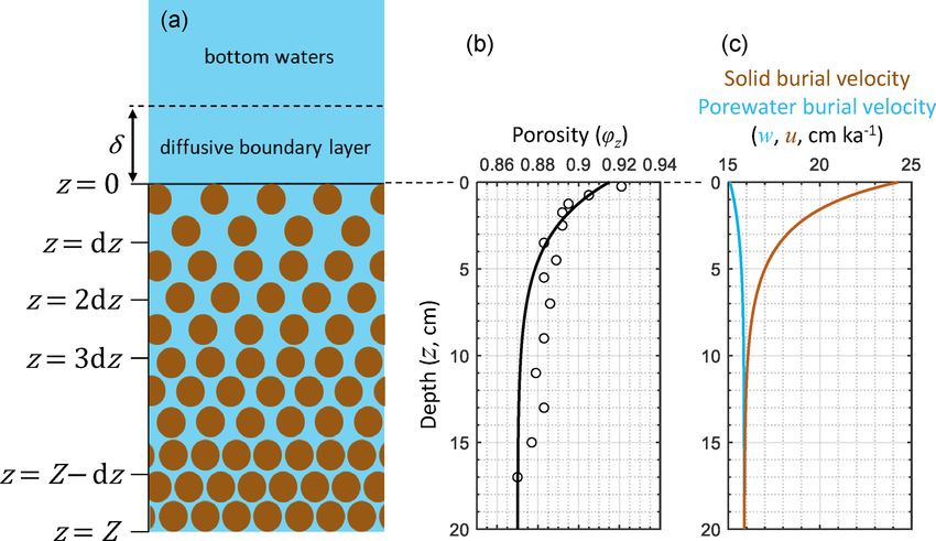
O. Sulpis et al.: RADIv1 2107
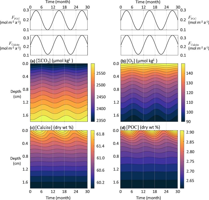
Figure 1. Schematic of RADI’s vertical structure alongside steady-state depth profiles of porosity ϕz (see Eqs. 3 and 4), porewater (u, solid
light blue line) and solid (w, solid brown line) burial velocities at in situ conditions taken at station 7 of Sayles et al. (2001). Burial velocity
varies with depth due to porosity, as described in Sect. 2.3. The open circles in the porosity profile are porosity measurements from Sayles et
al. (2001).
clude an inventory of model variables and parameters and a few days to study the response of the sedimentary system
list of nomenclature for chemical species, respectively. to high-frequency cyclic phenomena such as tides. For ini-
tial conditions, the user can choose between predefined uni-
2.1 Model structure and fundamental equation form values (e.g., set all concentrations to zero) or a set of
saved concentrations (e.g., from a previous simulation that
RADI uses the same set of reactive-transport partial differen- has reached steady state). T is the total simulation time, dt is
tial equations as implemented in CANDI (Boudreau, 1996b), the temporal resolution, i.e., the interval between each time
i.e., for each solute component, step, and t refers to the array of modeled time points. All
time units are in years (a). The interface between the sur-
∂ν 1 ∂ ∂ν X
= ϕd − ϕuν + α(vw − v) + R, (1) face sediment and overlying seawater, conventionally set at
∂t ϕ ∂z ∂z a sediment depth z = 0, represents the top layer of RADI’s
and for each solid component, vertical axis (Fig. 1). The bottom layer of the model is at a
sediment depth Z. Between these limits, n layers are present,
each being separated by a constant vertical gap dz. Depth
X
∂ν 1 ∂ ∂ν
= ϕs b − ϕs wν + R, (2) units are in meters. The values assigned to dz and dt depend
∂t ϕs ∂z ∂z
on the nature of the problem and on the kinetics of the chem-
where v is the concentration of a given component, t is time, ical reactions. In the present study, all cases use dz = 2 mm
ϕ is sediment porosity, ϕs is the solid–volume fraction, d is and dt = 1/128 000 a, i.e., ∼ 4 min. If a lower dz is used, dt
the effective molecular diffusion coefficient, b is the biotur- needs to be lowered as well to preserve numerical stability.
bation coefficient, z is depth, u is the porewater burial ve- In general, the ratio dz/dt should be kept below a value of
locity, w is the solid burial velocity, α is the irrigation coeffi- 256 m a−1 . If dz is divided by two, dt needs to be divided
cient, vw is the concentration of a solute in the bottom waters, by two as well, and the speed at which RADI runs will be
and 6R is the net production rate from all biogeochemical reduced by a factor of four.
reactions for a given component. Each of these terms will RADI operates on a static, user-defined porosity profile.
be described in detail later in this section. These partial dif- Sediment porosity, ϕz in Fig. 1, refers to the porewater vol-
ferential equations are solved numerically using the method ume fraction in the sediment (dimensionless) and typically
of lines described in Boudreau (1996b). Instead of search- decreases exponentially with sediment depth due to steady-
ing for steady-state solutions directly, RADI computes the state compaction. The sediment porosity profile is parame-
concentrations of a set of solids and solutes at each depth terized following Boudreau (1996b) as follows:
and time step following a time vector set by the user. The
user determines the simulation time depending on the ob-
jectives, e.g., multimillennial to predict a steady state, or a ϕz = ϕ∞ + (ϕ0 − ϕ∞ )e−βz , (3)
https://doi.org/10.5194/gmd-15-2105-2022 Geosci. Model Dev., 15, 2105–2131, 2022
2108                                                                                                       O. Sulpis et al.: RADIv1

Table 1. Nomenclature of model parameters and variables.

              Variable     Model notation        Description                                               Equation no.
              General
              Z            z_max                 Total height of the sediment column
              dz           z_res                 Depth resolution
              z            depths                Array of modeled depths within the sediment
              T            stoptime              Total simulation time
              dt           interval              Time steps
              t            timesteps             Array of modeled time points
              ϕz           phi                   Porewater porosity                                        3
              β            phiBeta               Porosity attenuation coefficient                          3
              ϕs,z         phiS                  Solid volume fraction                                     4
              θ2           tort2                 Squared tortuosity                                        24
              Fv           Fvar                  Solid deposition flux
              vw           var_w                 Bottom waters solute concentration
              δ            dbl                   Diffusive boundary layer thickness
              Tw           T                     Temperature
              Advection
              u            u                     Porewater burial velocity                                 17
              w            w                     Solid burial velocity                                     15, 16, 18
              Peh,z        Peh                   Half of the cell Péclet number                            22
              σz           sigma                 Number from Fiadero and Veronis (1977)                    21
              Reactions
              c/p          RC                    Redfield ratio for carbon
              n/p          RN                    Redfield ratio for nitrogen
              p/p          RP                    Redfield ratio for phosphorus
              Kv           Kvar                  Half-saturation constant for a given electron acceptor
              Kv0          Kvari                 Inhibition constant for a given electron acceptor
              kreaction    kvar                  Rate constant for a given chemical reaction
              fv,z         fvar                  Fractions of organic matter degraded by a given oxidant   7, 8
              ηdiss. ca.   order_diss_ca         Reaction order for calcite dissolution                    12
              ηdiss. ar.   order_diss_ar         Reaction order for aragonite dissolution                  13
              ηprec. ca.   order_prec_ca         Reaction order for calcite precipitation                  14
              ca          OmegaCa               Seawater saturation state with respect to calcite         12, 14
              ar          OmegaAr               Seawater saturation state with respect to aragonite       13
              Diffusion
              dz (v)       D_var_tort2           Effective molecular diffusion coefficient                 23, 27
              dz ◦ (v)     D_var                 Free-solution molecular diffusion coefficient             23
              bz           D_bio                 Bioturbation coefficient                                  25, 26
              λb           lambda_b              Characteristic bioturbation depth                         26
              Irrigation
              αz           alpha                 Irrigation coefficient                                    30, 31
              λi           lambda_i              Characteristic depth for irrigation                       31

where ϕ∞ is the porosity at great depth, ϕ0 is the porosity at        fraction (ϕs , dimensionless) is defined as follows:
the sediment–water interface, and β is an attenuation coeffi-
                                                                      ϕs,z = 1 − ϕz ,                                           (4)
cient (in m−1 ). A typical deep-sea sediment porosity profile
is shown in Fig. 1. Here the measured porosity profile at sta-        and increases with sediment depth (as compaction forces
tion 7 of cruise NBP98-2 (Sayles et al., 2001) is fit using           squeeze porewaters out).
ϕ∞ = 0.87, ϕ0 = 0.915, and β = 33 m−1 . The solid volume                Within this grid and for each time step, RADI com-
                                                                      putes the concentrations of 11 solute variables (TAlk, 6CO2 ,

Geosci. Model Dev., 15, 2105–2131, 2022                                                 https://doi.org/10.5194/gmd-15-2105-2022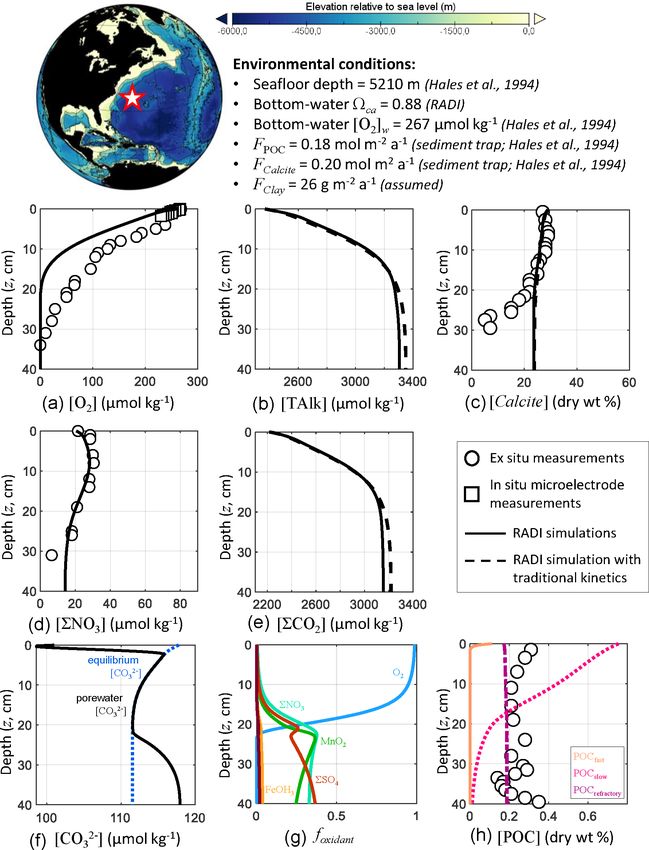
O. Sulpis et al.: RADIv1                                                                                                                           2109

Table 2. Nomenclature of modeled chemical species. All variables are concentrations, expressed in mol per cubic meter of solid for solid
species and mol per cubic meter of water for solute species.

                                   Variable v                  Model notation         Description
                                   [O2 ]                       dO2                    Dissolved oxygen
                                   [TAlk]                      dalk                   Total alkalinity
                                   [6CO2 ]                     dtCO2                  Dissolved inorganic carbon
                                   [Ca2+ ]                     dCa                    Dissolved calcium
                                   [6NO3 ]                     dtNO3                  Dissolved inorganic nitrogen
                                   [6SO4 ]                     dtSO4                  Dissolved inorganic sulfate
                                   [6PO4 ]                     dtPO4                  Dissolved inorganic phosphorus
                                   [6NH4 ]                     dtNH4                  Dissolved inorganic nitrogen
                                   [6H2 S]                     dtH2S                  Dissolved inorganic sulfide
                                   [Fe2+ ]                     dFe                    Dissolved iron
                                   [Mn2+ ]                     dMn                    Dissolved manganese
                                   [POCrefractory ]            proc                   Refractory particulate organic carbon
                                   [POCslow ]                  psoc                   Slow-decay particulate organic carbon
                                   [POCfast ]                  pfoc                   Fast-decay particulate organic carbon
                                   [Calcite]                   pcalcite               Calcite
                                   [Aragonite]                 paragonite             Aragonite
                                   [MnO2 ]                     pMnO2                  Manganese (IV) oxide
                                   [Fe(OH)3 ]                  pFeOH3                 Iron (III) hydroxide
                                   [Clay]                      pclay                  Clay∗
                                 ∗ We consider all clay minerals to be montmorillonite (Al H O Si ; molar mass is equal to
                                                                                          2 2 12 4
                                 360.31 g mol−1 ).

O2 , Ca2+ , 6NO3 , 6SO4 , 6PO4 , 6NH4 , 6H2 S, Fe2+ , and                              are grouped into three categories: (i) organic matter degra-
Mn2+ ) and 8 solid variables (Calcite, Aragonite, Fe(OH)3 ,                            dation, (ii) oxidation of reduced metabolites (organic matter
MnO2 , Clay, and three kinds of particulate organic carbon,                            degradation byproducts), and (iii) dissolution or precipitation
collectively termed POC). Note that clay is simply modeled                             of calcium carbonate minerals. RADI has been designed for
as a non-reactive solid that is included because the clay ac-                          early diagenesis in deep-sea sediments, and thus formation
cumulation flux to the sediment–water interface participates                           and re-oxidation of metal sulfide minerals are not considered.
in the calculation of the solid burial velocity; see Sect. 2.3.
Concentration units are in mol per square meter of water for                           2.2.1     Organic matter degradation
solutes and in mol per square meter of solid for solid species.
For each modeled solute or solid concentration v at time t                             Organic carbon deposited on the seafloor originates mainly
and sediment depth z, the following equation applies:                                  from primary production in the upper ocean or on land and
                                                                                       (to a lesser extent) from the ocean interior via chemoautotro-
v(t+dt),z = vt,z + [R(vt,z ) + A(vt,z ) + D(vt,z ) + I (vt,z )] · dt ,      (5)        phy. Despite the differences in origin, detrital organic matter
where R(vt,z ) quantifies the rate of change of vt,z due to                            found in marine sediments typically has the same composi-
chemical reactions, A(vt,z ) quantifies the rate of change of                          tion: ∼ 60 % proteins, ∼ 20 % lipids, ∼ 20 % carbohydrates,
vt,z due to advection, D(vt,z ) quantifies the rate of change of                       and a fraction of other compounds (Hedges et al., 2002; Bur-
vt,z due to molecular and bio-diffusion, and I (vt,z ) quanti-                         dige, 2007; Middelburg, 2019). Here, the stoichiometry of or-
fies the rate of change of vt,z due to bio-irrigation. In general,                     ganic matter is represented by the coefficients c (for carbon),
only the subscript z variables are explicitly written out in this                      n (for nitrogen), and p (for phosphorus). By default, the c : p
paper for variables and parameters that vary with depth. The                           ratio is set to 106 : 1 and the n : p ratio set to 16 : 1, follow-
t variables are implicit but excluded for clarity.                                     ing the Redfield ratio that describes the average composition
                                                                                       of phytoplankton biomass (Redfield, 1958), but these values
2.2    Reactions                                                                       can easily be adjusted. In RADI, c/p is denoted RC, n/p
                                                                                       is denoted RN, and p/p is denoted RP, which is unity. Or-
In RADI, biogeochemical reactions operate on solutes and                               ganic matter is also simplified here as an elementary carbo-
solids throughout the entire sediment column, including the                            hydrate (CH2 O). In reality, loss of H and O during biosynthe-
very top and bottom layers. R(vz ) is the net rate at which vz                         sis of proteins, lipids, and polysaccharides occurs (Anderson,
is being consumed (negative R) or produced (positive R) by                             1995; Hedges et al., 2002; Middelburg, 2019), which results
these reactions. Biogeochemical reactions in RADI (Table 3)                            in an effective molar ratio of O2 consumed to C degraded of

https://doi.org/10.5194/gmd-15-2105-2022                                                                       Geosci. Model Dev., 15, 2105–2131, 2022
2110                                                                                                                      O. Sulpis et al.: RADIv1

Table 3. Diagenetic reactions, reaction rates, and reaction contributions to porewater.

 Reaction                                                          Rate [mM a−1 ]                                         1TAlk                 16CO2
 Organic matter degradation
 (CH2 O)(NH3 ) n (H3 PO4 ) p + O2                                  (kPOCfast [POCfast ] + kPOCslow [POCslow ])fO2         +n/c − p/c                 +1
                c          c
 ↔ CO2 + nc NH3 + pc H3 PO4 + H2 O
 (CH2 O)(NH3 ) n (H3 PO4 ) p + 0.8 NO3 −                           (kPOCfast [POCfast ] + kPOCslow [POCslow ])f6NO3       +0.8 + n/c − p/c           +1
                c          c
 ↔ 0.2 CO2 + 0.4 N2 + 0.8 HCO3 − + nc NH3 + pc H3 PO4 + 0.6 H2 O
 (CH2 O)(NH3 ) n (H3 PO4 ) p + 2 MnO2 + 3 CO2 + H2 O               (kPOCfast [POCfast ] + kPOCslow [POCslow ])fMnO2       +4 + n/c − p/c             +1
                c          c
 ↔ 4 HCO3 − + 2 Mn2+ + nc NH3 + pc H3 PO4
 (CH2 O)(NH3 ) n (H3 PO4 ) p + 4 Fe(OH)3 + 7 CO2                   (kPOCfast [POCfast ]+kPOCslow [POCslow ])fFe(OH)3      +8 + n/c − p/c             +1
               c           c
 ↔ 8 HCO3 − + 4 Fe2+ + nc NH3 + pc H3 PO4 + 3 H2 O
 (CH2 O)(NH3 ) n (H3 PO4 ) p + 0.5 SO4                             (kPOCfast [POCfast ] + kPOCslow [POCslow ])f6SO4       +1 + n/c − p/c             +1
                c          c
 ↔ HCO3 − + 0.5 H2 S + nc NH3 + pc H3 PO4
 (CH2 O)(NH3 ) n (H3 PO4 ) p                                       (kPOCfast [POCfast ] + kPOCslow [POCslow ])fCH4        +n/c − p/c               +0.5
                c          c
 ↔ 0.5 CO2 + 0.5 CH4 + nc NH3 + pc H3 PO4
 Redox reactions
 Fe2+ + 0.25 O2 + 2 HCO3 − + 0.5 H2 O ↔ Fe(OH)3 + 2 CO2            kFe ox [Fe2+ ][O2 ]                                    −2                           0
 Mn2+ + 0.5 O2 + 2 HCO3 − ↔ MnO2 + 2 CO2 + H2 O                    kMn ox [Mn2+ ][O2 ]                                    −2                           0
 H2 S + 2 O2 + 2 HCO3 − ↔ SO4 2− + 2 CO2 + 2 H2 O                  kS ox [6H2 S][O2 ]                                     −2                           0
 NH3 + 2 O2 + HCO3 − ↔ NO3 − + CO2 + 2 H2 O                        kNH ox [6NH4 ][O2 ]                                    −2                           0
 CaCO3 dissolution and precipitation
 CaCO3 ↔ Ca2+ + CO3 2−                                             [Calcite] · kdiss. ca. · (1 − ca )ηdiss. ca.          +2                         +1
 CaCO3 ↔ Ca2+ + CO3 2−                                             [Aragonite] · kdiss. ar. · (1 − ar )ηdiss. ar.        +2                         +1
 Ca2+ + CO3 2− ↔ CaCO3                                             kprec. ca. · (ca   − 1)ηprec. ca.                     −2                         −1

∼ 1.2 during aerobic respiration (Anderson and Sarmiento,                     tion rate decreases with depth because the quantity of or-
1994) instead of 1 as assumed here (Table 3).                                 ganic matter and the relative proportions of fast- and slow-
   Observations show that some organic compounds are pref-                    decay materials decline with depth. Organic matter is de-
erentially degraded and become selectively depleted (Cowie                    graded following the sequential utilization of available ox-
and Hedges, 1994; Lee et al., 2000). As a result, the bulk                    idants. The oxidant limitation is represented by a Michaelis–
reactivity of organic matter decreases with increasing age                    Menten-type (also termed “Monod”) function, in which each
(Middelburg, 1989). Degradation of organic matter deposited                   oxidant has an associated half-saturation constant (Koxidant in
at the seafloor typically follows a sequential utilization of                 mol m−3 ) that symbolizes the oxidant concentration at which
available oxidants, O2 , NO3 − , MnO2 , Fe(OH)3 , and SO4 2− ,                the process proceeds at half its maximal speed (Soetaert et
followed by methanogenesis (Froelich et al., 1979; Berner,                    al., 1996b). The presence of some oxidants may also inhibit
1980; Arndt et al., 2013). All organic matter degradation re-                 other metabolic pathways; this is represented by an inhibi-
actions implemented in RADI are shown in Table 3.                                                0
                                                                              tion constant (Koxidant  in mol m−3 ) that is specific to each
   To account for the decrease in organic matter degrada-                     oxidant. These limiting and inhibitory functions have been
tion rate with sediment depth, we separate organic matter                     widely used (Boudreau, 1996b; Van Cappellen and Wang,
into fractions of different reactivity, and we assign a rate                  1996; Soetaert et al., 1996b; Couture et al., 2010), they allow
constant to each of the degradable fractions. Following Jør-                  a single equation to be used for each component across the
gensen (1978), Westrich and Berner (1984), and Soetaert et                    entire model depth range, and they also permit some over-
al. (1996b), three different classes of organic matter are con-               lap between the different pathways, as observed in nature
sidered: refractory, slow-decay, and fast-decay organic mat-                  (Froelich et al., 1979). In RADI, the overall degradation of
ter. The refractory organic matter class is not reactive during               fast- or slow-decay organic carbon occurs at the following
the timescales considered here. The fast- and slow-decay or-                  rate:
ganic matter fractions each have a depth-dependent, oxidant-
independent reactivity. The overall organic matter degrada-                   RPOCfast or slow ,z = foxidant,z · kPOCfast or slow · [POCfast or slow ]z (6)

Geosci. Model Dev., 15, 2105–2131, 2022                                                                 https://doi.org/10.5194/gmd-15-2105-2022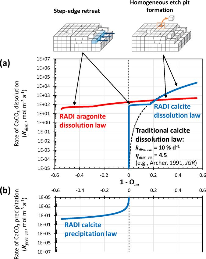
O. Sulpis et al.: RADIv1                                                                                                              2111

where kPOC is the rate constant for the degradation of a given            numbers 1.3 × 10⁻⁴ and 1.5 × 10⁻¹ have been tuned to best
type of organic carbon (fast- or slow-decay types, expressed              fit observations of both a Southern Ocean station and a North
in a−1 ), [POCfast or slow ] is the concentration of organic car-         Atlantic station; see Sect. 3.
bon (fast- or slow-decay) in sediments, and fOx. is the sum
of the fractions of organic carbon degraded by each oxidant               2.2.2   Oxidation of organic matter degradation
(dimensionless, always equal to one), given by                                    by-products
foxidant,z = fO2 ,z + f6NO3 ,z + fMnO2 ,z + fFe(OH)3 ,z
                                                                          Organic matter degradation reactions primarily change oxi-
            + f6SO4 ,z + fCH4 ,z ,                                  (7)   dants (e.g., O2 , NO3 − , MnO2 , Fe(OH)3 , SO4 2− ) into their
where                                                                     reduced forms (e.g., H2 O, N2 , Mn2+ , Fe2+ , H2 S; Table 3). If
              [O2 ]z                                                      oxygen is introduced into the system or the reduced metabo-
     fO2 ,z =            ,                                         (8a)   lites diffuse upwards in oxic porewaters, then these reduced
            KO2 + [O2 ]z
                                                                          byproducts are converted back into their oxidized form and
                [6NO3 ]z                                                  the energy contained in them becomes available to the micro-
 f6NO3 ,z =
            K6NO3 + [6NO3 ]z                                              bial community, though these energetics are not considered
                 KO0 2                                                    in RADI.
            × 0            ,                                       (8b)      Here, four redox reactions involving organic matter degra-
             KO2 + [O2 ]z
                                       0
                                                                          dation byproducts are implemented (Table 3): oxidation of
                   [MnO2 ]z          K6NO  3                              Fe2+ , Mn2+ , 6H2 S, and 6NH3 , respectively. These four
  fMnO2 ,z =                      0
                KMnO2 + [MnO2 ]z K6NO3
                                       + [6NO 3 ]z                        reactions consume porewater total alkalinity (TAlk) but do
                        KO0 2                                             not alter porewater 6CO2 (Table 3), thus locally acidify-
                ×                    ,                             (8c)   ing porewaters. Here, we use the TAlk definition of Dickson
                    KO0 2 + [O2 ]z                                        (1981), in which TAlk is defined as “the number of moles
                                             0
                                           KMnO                           of hydrogen ion equivalent to the excess of proton accep-
                     [Fe(OH)3 ]z                 2
fFe(OH)3 ,z =                           0                                 tors (bases formed from weak acids with a dissociation con-
                KFe(OH)3 + [Fe(OH)3 ]z KMnO  + [MnO2 ]z
                                           2                              stant K ≤ 10−4.5 and zero ionic strength) over proton donors
                           0
                          K6NO                    KO0 2
                              3                                           (acids with K > 10−4.5 ) in one kilogram of sample.” This
                ×    0                                         ,   (8d)
                    K6NO 3
                           + [6NO3 ]z KO0 2 + [O2 ]z                      scheme should be sufficient for all open-ocean applications
                                           0                              but may not be suitable for coastal and anoxic environments
                   [6SO4 ]z            KFe(OH)
  f6SO4 ,z =                                    3                         with extensive metal sulfide mineral turnover, which require
                                  0
                K6SO4 + [6SO4 ]z KFe(OH)   + [Fe(OH)
                                         3
                                                    3 ]z                  a more complete set of redox reactions such as that from the
                           0
                          KMnO                         0
                                                      K6NO                CANDI model of Boudreau (1996b). Additional components
                               2                           3
                ×    0                 0                                  and reactions can easily be implemented in future versions
                    KMnO   + [MnO2 ]z K6NO   + [6NO3 ]z
                         2                 3                              (see Sect. 5). The rate constants for these four redox reactions
                        KO0 2                                             are taken from Boudreau (1996b) and reported in Table 4.
                ×                    ,                             (8e)
                    KO0 2 + [O2 ]z
                         0                         0                      2.2.3   CaCO3 dissolution and precipitation
                        K6SO 4
                                                  KFe(OH)3
   fCH4 ,z =     0                 0
                K6SO 4
                       + [6SO4 ]z KFe(OH) 3
                                            + [Fe(OH)3 ]z                 RADI includes two CaCO3 polymorphs: low Mg calcite and
                           0
                          KMnO                         0
                                                      K6NO                aragonite, but more could be added in future versions, e.g.,
                               2                           3
                ×    0                 0                                  high Mg calcite and/or vaterite. Calcite and aragonite both
                    KMnO   + [MnO2 ]z K6NO   + [6NO3 ]z
                         2                 3                              have different dissolution kinetics, in which their dissolu-
                        KO0 2                                             tion rates increase as the undersaturation state of seawater
                ×                    .                             (8f)   with respect to calcite (1 − ca,z ) or aragonite (1 − ar,z ) in-
                    KO0 2 + [O2 ]z
                                                                          creases (Keir, 1980; Walter and Morse, 1985; Sulpis et al.,
Half-saturation and inhibition constants for each oxidant                 2017; Dong et al., 2019; Naviaux et al., 2019b). Here, z
used in RADI are given in Table 4. The degradation rate con-              is the sediment-depth-dependent saturation state of seawater
stant of organic carbon, kPOCfast or slow , is computed as a func-        with respect to calcite or aragonite, computed as [Ca2+ ]z ·
tion of the flux of organic carbon reaching the seafloor and is           [CO3 2− ]z /Ksp
                                                                                        ∗ , where K ∗ is the stoichiometric solubility
                                                                                                     sp
sediment depth dependent (Archer et al., 2002):                           constant of calcite or aragonite at in situ temperature, pres-
kPOCfast = (1.5 × 10⁻¹ )(FPOC · 102 )0.85 ,                        (9a)   sure, and salinity, as given in Mucci (1983) and Millero
                         −4              2 0.85                           (1995). At each time step, z is computed using porewater
kPOCslow = (1.3 × 10          )(FPOC · 10 )       ,                (9b)
                                                                          [Ca2+ ]z and [CO3 2− ]z from the previous time step, the latter
where FPOC is the total flux of organic carbon reaching the               being calculated as a function of TAlk and the proton con-
seafloor (i.e., fast, slow, and refractory, in mol m−2 a−1 ). The         centration [H+ ]. At each model time step, the total hydrogen

https://doi.org/10.5194/gmd-15-2105-2022                                                     Geosci. Model Dev., 15, 2105–2131, 2022
2112 O. Sulpis et al.: RADIv1
Table 4. Suggested values for model parameters.
Parameter Model notation Value Unit Source
KO2 /KO0 KdO2/KdO2i 3/10 µM Soetaert et al. (1996b)
2
K6NO3 /K6NO0 KdtNO3/KdtNO3i 30/5 µM Soetaert et al. (1996b)
3
KMnO2 = KMnO 0 KpMnO2/KpMnO2i 42.4 mM Van Cappellen and Wang (1996)1
2
0
KFe(OH)3 = KFe(OH) KpFeOH3/KpFeOH3i 265 mM Van Cappellen and Wang (1996)1
3
K6SO4 = K6SO 0 KdtSO4/KdtSO4i 1.6 mM Van Cappellen and Wang (1996)1
4
kFe ox kFeox 106 mM−1 a−1 Boudreau (1996b)2
kMn ox kMnox 106 mM−1 a−1 Boudreau (1996b)2
kS ox kSox 3 ×10⁵ mM−1 a−1 Boudreau (1996b)2
kNH ox kNHox 104 mM−1 a−1 Boudreau (1996b)2
β phiBeta 33 m−1 Tuned
λb lambda_b 0.08 m Archer et al. (2002)
λi lambda_i 0.08 m Archer et al. (2002)
1 Assuming a solid density of 2.65 g cm−3 . 2 Values for the “deep sea”.
ion concentration [H+ ] is computed from TAlk and CO2
P
have previously been implemented to describe calcite disso-
using a single Newton–Raphson iteration from the previous lution rates (e.g., Archer et al., 2002) but in most cases used
time step (Humphreys et al., 2022): a high reaction order and a tuned rate constant independent
of solution chemistry (Fig. 2). Such discretizations are con-
[H+ ]t = [H+ ]t−1 venient but lack a mechanistic description of the controls on
[TAlk]([H+ ]t−1 , [ CO2 ]) − [TAlk] calcite dissolution in seawater (Adkins et al., 2021).
P
− , (10) The latest advances using isotope-labeling approaches to
d[TAlk]([H+ ]t−1 , [ CO2 ])/d[H+ ]t−1
P
study carbonate dissolution kinetics show abrupt changes
where [H+ ]t is the new [H+ ] value and [H+ ]t−1 + in dissolution mechanism depending on solution saturation
P is the [H ]
+
from the previous time step. TAlk([H ]t−1 , CO2 ) is the state with either calcite or aragonite (Subhas et al., 2017;
total alkalinity Dong et al., 2019; Naviaux et al., 2019a, b). Close to equi-
P computed from user-specified total dissolved
silicate, [ PO4 ] and total borate calculated from salinity librium, dissolution occurs primarily at sites on the crystal
(Uppström, 1974), plus equilibrium constants for silicic acid surfaces that are most exposed to the solution, e.g., steps
(Sillén et al., 1964) and phosphoric acid (Yao and Millero, and kinks. Further away from equilibrium, dissolution etch
1995). Its derivative is computed following the approach of pits are activated at surface sites associated with defects and
CO2SYS; see Humphreys et al. (2022). The carbonate ion impurity atoms. Far away from equilibrium, there is enough
concentration is then computed as follows: free energy for dissolution etch pits to occur anywhere on
the mineral surface, without the aid of crystal defects (Ad-
[ CO2 ] × K1∗ × K2∗
P
2− kins et al., 2021). However, at temperatures most relevant
[CO3 ] = ∗ , (11)
K1 × K2∗ + K1∗ × [H+ ]t + [H+ ]2t to the deep oceans, ∼ 5 ◦ C or less, the defect-assisted dis-
solution mechanism is skipped (Naviaux et al., 2019b) and
where K1∗ and K2∗ are the first and second dissociation con- only the step-edge retreat (close to equilibrium) and homo-
stants for carbonic acid, respectively, taken from Lueker et geneous etch-pit formation (far away from equilibrium) dis-
al. (2000). solution regimes remain (Naviaux et al., 2019b) (Fig. 2). For
The dissolution rates (Rdiss , in mol m−3 a−1 ) of calcite both aragonite and calcite, while homogeneous etch-pit for-
(solid blue line in Fig. 2a) and of aragonite (solid red line mation is indeed associated with a high-order dependency
in Fig. 2a) as a function of (1 − ca ) are empirically defined on the solution saturation state, step-edge retreat dissolu-
as follows: tion rates dominating near equilibrium show very little de-
pendence on seawater saturation (Dong et al., 2019; Navi-
Rdiss. ca.,z = [Calcite] · kdiss. ca. · (1 − ca )ηdiss. ca. , (12) aux et al., 2019a). This could have significant consequences
ηdiss. ar. for the predicted carbonate dissolution rate near equilib-
Rdiss. ar.,z = [Aragonite] · kdiss. ar. · (1 − ar ) . (13)
rium: saturation-state-independent step-edge retreat dissolu-
In these expressions, the dissolution rate constant (kdiss , in tion will always be predicted to be faster close to equilib-
a−1 ) and the reaction order (ηdiss , unitless) are mineral spe- rium than dissolution associated with a high reaction order
cific. The dissolution rate constants implicitly account for because a high reaction order forces the dissolution rate to
each mineral’s specific surface area. Similar formulations
Geosci. Model Dev., 15, 2105–2131, 2022 https://doi.org/10.5194/gmd-15-2105-2022O. Sulpis et al.: RADIv1 2113
tuned to best fit the observations in the two stations presented
in Sect. 3. We use kdiss. ca. = 6.3 × 10⁻³ a−1 for 0.828 <
ca < 1, kdiss. ca. = 20 a−1 for ca ≤ 0.828, kdiss. ar. = 3.8 ×
10−3 a−1 for 0.835 < ar < 1, and kdiss. ar. = 4.2 × 10⁻² a−1
for ar ≤ 0.835. Both calcite and aragonite dissolution rate
constants are lower than the values reported in the orig-
inal publications. We suspect that (i) the reactive surface
area of grains in sediments is much smaller than their spe-
cific surface area measured using adsorption isotherms via
the Brunauer–Emmett–Teller (BET) method and (ii) unac-
counted dissolution inhibitors are present in sediments, such
as dissolved organic carbon (Naviaux et al., 2019a). A com-
parison of the steady-state [CO3 2− ] and [Calcite] porewater
profiles predicted by RADI using the tuned rate constants
implemented in RADIv1 and the original rate constants is
shown in Fig. S1 in the Supplement.
Calcite precipitation is also included in the model and its
rate (solid blue line in Fig. 2b) is parameterized with the fol-
lowing function:
Rprec. ca.,z = kprec. ca. · (ca − 1)ηprec. ca. , (14)
where kprec. ca is the precipitation rate constant set to
0.4 mol m−3 a−1 and η is equal to 1.76. The precipitation re-
action order is taken from Zuddas and Mucci (1998), cor-
rected for a seawater-like ionic strength of 0.7 mol kg−1 . The
Figure 2. (a) Dissolution rate of calcite as computed using Eq. (12) precipitation and dissolution rate continuum implemented in
and [Calcite] = 104 mol m−3 (solid blue line), and dissolution RADI (see Fig. 2) is very different from what a classic model
rate of aragonite as computed using Eq. (13) and [Aragonite] = with only calcite dissolution following high reaction order ki-
104 mol m−3 (solid red line). Note that for each dissolution rate pro- netics would display. For comparison, the dissolution rate of
file, two different rate constants (kdiss ) and reaction orders (ηdiss ) calcite using a dissolution rate constant kdiss of 10 % d−1 and
are used, depending on the seawater saturation state, with each ac-
a reaction order η of 4.5, as implemented in most diagenetic
counting for a separate dissolution mechanism, i.e., step-edge re-
treat or homogeneous-edge pit formation. The dashed black line
models, including Archer (1991), is shown in Fig. 2a. The
stands for a “traditional” dissolution rate profile obtained using value of 10 % d−1 for the rate constant was chosen because it
[Calcite] = 104 mol m−3 , a single dissolution rate constant for the makes the “traditional” calcite dissolution law overlap with
entire (1 − ca ) range kdiss = 10 % d−1 , and a reaction order ηdiss the RADI dissolution law so that any differences between
of 4.5. (b) Precipitation rate of calcite as computed from Eq. (14). the two can be attributed to enhanced dissolution caused by
Note that dissolution rates are normalized here per total solid sed- step-edge retreat close to equilibrium. Mechanistic interpre-
iment volume and not per CaCO3 surface area as in traditional ki- tations of the “kinks” in the dissolution rate profiles and of a
netics studies. non-zero dissolution rate near equilibrium still require more
research, but the implications of these features for our under-
standing of marine CaCO3 cycles can be explored with the
converge to zero as the solution gets closer to equilibrium present model.
(Fig. 2).
Naviaux et al. (2019a) derived reaction orders for two 2.3 Advection
separate regions of the (1 − ca ) spectrum: the ca thresh-
The solid burial velocity at the sediment–water interface, w0
old value dividing these two regions was ca. critical ≈ 0.8.
in m a−1 , is given by
Here, based on the results of Naviaux et al. (2019a), we
set ηdiss. ca. = 0.11 for 0.828 < ca < 1 and ηdiss. ca. = 4.7 for X Fv · Mv .
ca ≤ 0.828. The ca critical value used here is slightly higher w0 = ϕs,0 , (15)
ρv
than the ∼ 0.8 value given in Naviaux et al. (2019a) in order
to have a smooth transition between defect-assisted and ho- where Fv is the flux of a solid species at the sediment–water
mogeneous dissolution. For aragonite, based on the results of interface (mol m−2 a−1 ), Mv is the molar mass of that solid
Dong et al. (2019), we set ηdiss. ar. = 0.13 for 0.835 < ar < (g mol−1 ), and ρv is its solid density (g m−3 ). The solid and
1 and ηdiss. ar. = 1.46 for ar ≤ 0.835. The rate constants are porewater burial velocity at greater depth are assumed to be
https://doi.org/10.5194/gmd-15-2105-2022 Geosci. Model Dev., 15, 2105–2131, 20222114 O. Sulpis et al.: RADIv1
equal and are computed as follows: 2.4 Diffusion
w∞ = u∞ = w0 ϕs,0 /ϕs,∞ . (16) The diffusion flux of any species depends on its effective dif-
Thus, the porewater burial velocity, u, at all depths is fusion coefficient, dz (v), which varies with depth within the
sediment.
uz = u∞ ϕ∞ /ϕz , (17) For each solute, free-solution diffusion coefficients, de-
and the solid burial velocity, w, is noted dz ◦ (v), were computed at in situ temperatures (Li and
Gregory, 1974; Boudreau, 1997; Schulz, 2006). For solute
wz = w∞ ϕs,∞ /ϕs,z . (18) variables representing several individual species (e.g., 6PO4 ,
Depth profiles of u and w are shown in Fig. 1, computed from 6CO2 ), the diffusion coefficient of the dominant species was
the solid fluxes at station 7 of cruise NBP98-2 (Sayles et al., considered. Given the high proportion of HCO3 − relative to
2001); see Sect. 3.2. In Fig. 1, the sharp porosity decline in CO3 2− and CO2 (aq) in seawater and porewaters (see Fig. S2
the top centimeters of the sediments causes the solid fraction in the Supplement), the diffusion coefficient of HCO3 − was
at ∼ 5 cm depth to be roughly 50 % higher than just below adopted for both TAlk and 6CO2 . However, this approach
the interface. This leads to a solid burial velocity decrease of may not be suited for sedimentary environments in which pH
about the same magnitude (Fig. 1). is lower than 7 because a greater proportion of dissolved inor-
Advection is implemented following Boudreau (1996b), ganic species would then be under the form of carbonic acid,
where the advection rate (Az , in mol m−3 a−1 ) for solutes is i.e., CO2 (aq) , which has a higher diffusion coefficient than
given by HCO3 − (Fig. S2). Free-solution diffusion coefficients, their
! temperature dependencies, and their sources are reported in
dz (v) dϕz ◦ d 1/θz2 Table 5. The diffusion of solutes in the porewaters is slower
Az (v) = − uz − · − d (v) · than in an equivalent volume of water as a result of the phys-
ϕz dz dz
ical barriers caused by the presence of solid grains in a sedi-
v(z+dz ) − v(z−dz )
· , (19) ment. To correct for this effect, we follow Boudreau (1996b)
2dz and compute the effective diffusion coefficient for a given
where dz is the effective diffusion coefficient for a given so- solute as follows:
lute at a given depth (in m2 a−1 ), d◦ is the “free-solution”
dz (v) = d ◦ (v) θz2 ,
molecular diffusion coefficient for a given solute (in m2 a−1 ), (23)
and θz is the depth-dependent tortuosity (unitless) defined
in Sect. 2.4. For solids, a more sophisticated weighted- where so-called tortuosity (θ ) is defined as follows
difference scheme is employed (Fiadeiro and Veronis, 1977; (Boudreau, 1996a):
Boudreau, 1996b): p
θz = 1 − 2 ln (ϕz ) . (24)
dbz bz dϕs,z
Az (v) = − wz − − ·
dz ϕs,z dz
For each solid, effective diffusion occurs through the mix-
(1 − σz )v(z+dz) + 2σz vz − (1 + σz )v(z−dz)
· , (20) ing action of burrowing microorganisms, quantified using a
2dz bioturbation coefficient that decreases with depth. Archer et
where bz is the depth-dependent bioturbation coefficient al. (2002) used a dataset including 53 sediment sites ranging
(m2 a−1 ) and in depth from 47 to 5668 m to derive an optimal bioturbation
rate profile, in which the rate of bioturbation increases with
σz (v) = 1/ tanh(Peh,z ) − 1/Peh,z , (21)
increasing flux of total organic carbon reaching the seafloor
where (FPOC ) and attenuates in low-oxygen conditions. This pat-
tern was also observed by Smith et al. (1997) and Smith and
Peh,z = wz · dz/2bz . (22)
Rabouille (2002). As in Archer et al. (2002), we couple both
The parameter Peh is half of the cell Péclet number, which bioturbation and irrigation to the incoming carbon deposition
expresses the influence of advection relative to bioturbation flux (Fig. 3) rather than water depth or sediment accumula-
across a distance separating two points of the grid, centered tion rate (Boudreau, 1994; Middelburg et al., 1997; Soetaert
at the depth z. If bioturbation dominates (Peh
1), e.g., et al., 1996c), although all these quantities are related to each
near the sediment–water interface, σz tends toward zero and other. From an ecological perspective, more carbon to the
a centered-difference discretization is implemented. If ad- seafloor represents more food available to benthic commu-
vection dominates (Peh
1), e.g., deeper in sediments, σz nities, hence more biological transport. Linking bioturbation
tends toward unity and backward-difference discretization activity to carbon deposition flux also allows for a direct cou-
prevails; see Eq. (20). This differencing scheme, originally pling with Earth system models simulating carbon sinking
developed by Fiadeiro and Veronis (1977), maintains stabil- fluxes in the ocean. Following Archer et al. (2002), we ex-
ity in the entire sediment column (Boudreau, 1996b). press the surficial bioturbation mixing rate (b0 , in m2 a−1 ) as
Geosci. Model Dev., 15, 2105–2131, 2022 https://doi.org/10.5194/gmd-15-2105-2022O. Sulpis et al.: RADIv1 2115
Table 5. Temperature-dependent molecular diffusion coefficients (m2 a−1 ).
Diffusion coefficient Value Source
dz ◦ (TAlk) 0.015179 + 0.000795 × Tw Boudreau (1997), Schulz (2006)1
dz ◦ (6CO2 ) 0.015179 + 0.000795 × Tw Boudreau (1997), Schulz (2006)1
dz ◦ (Ca2+ ) 0.011771 + 0.000529 × Tw Li and Gregory (1974)
dz ◦ (O2 ) 0.031558 + 0.001428 × Tw Boudreau (1997), Schulz (2006)
dz ◦ (6NO3 ) 0.030863 + 0.001153 × Tw Li and Gregory (1974)2
dz ◦ (6SO4 ) 0.015779 + 0.000712 × Tw Li and Gregory (1974)3
dz ◦ (6PO4 ) 0.009783 + 0.000513 × Tw Boudreau (1997), Schulz (2006)4
dz ◦ (6NH4 ) 0.030926 + 0.001225 × Tw Li and Gregory (1974)5
dz ◦ (6H2 S) 0.028938 + 0.001314 × Tw Boudreau (1997), Schulz (2006)
dz ◦ (Fe2+ ) 0.001076 + 0.000466 × Tw Li and Gregory (1974)
dz ◦ (Mn2+ ) 0.009625 + 0.000481 × Tw Li and Gregory (1974)
1 value for HCO − ion, 2 Value for NO − ion. 3 Value for SO 2− ion. 4 Value for HPO 2− ion. 5 Value for NH +
3 3 4 4 4
ion.
follows: Aller, 2001). Mathematically, this is parameterized as a non-
local exchange function, i.e., a first-order kinetic reaction:
b0 = (2.32 × 10⁻⁶ )(FPOC × 102 )0.85 , (25)
It,z (v) = αz (vw − vz ) , (29)
where FPOC is expressed in mol m−2 a−1 . The bioturbation
mixing rate at all depths (bz , in m2 a−1 ) is where αz is an irrigation coefficient common to all solutes
(expressed in a−1 ). Following Archer et al. (2002), who
2 [O2 ]w
bz = b0 e−(z/λb ) , (26) used a dataset of 53 sediment sites comprised of microelec-
[O2 ]w + 0.02 trode oxygen profiles and chamber oxygen fluxes across the
where the characteristic depth λb = 8 cm, following Archer sediment–water interface to derive an irrigation rate profile,
et al. (2002), and [O2 ]w is the oxygen concentration in the we express the surficial irrigation coefficient as a function of
bottom waters. This depth-dependent bioturbation mixing the organic carbon deposition flux and the oxygen concentra-
rate is common to all solids, and its depth distribution is tion of the overlaying waters:
shown in Fig. 3 as a function of in situ [O2 ]w and FPOC . The 2 −400
effective diffusion coefficient for solids is then set as follows: tan−1 5FPOC ×10
400
α0 = 11 + 0.5 − 0.9
dz (v) = bz . (27) π
20[O2 ]w FPOC × 102 −[O2 ]w
+ · 2
· e 0.01 (30)
The (bio)diffusion is implemented in RADI following the [O2 ]w + 0.01 FPOC × 10 + 30
centered difference discretization scheme from Boudreau
and the irrigation coefficient at all depths as follows:
(1996b). At sediment depth z, where 0 < z < Z, for both so-
lutes and solids: 2
αz = α0 e−(z/λi ) , (31)
2
Dz (v) = dz (v) · (v(z−dz) − 2vz + v(z+dz) )/(dz) , (28)
where the characteristic depth λi is 5 cm (Archer et al., 2002).
where dz (v) is the relevant effective diffusion coefficient. The depth distribution of the irrigation coefficient is shown
in Fig. 3 as a function of in situ [O2 ]w and FPOC .
2.5 Irrigation
2.6 Boundary conditions
The mixing of solutes caused by burrow flushing or venti-
lation occurs through an ensemble of processes collectively Modeling of advection and diffusion processes requires ap-
termed irrigation. Macroscopic burrows are often present propriate boundary conditions in the layers above and below
in the seafloor sediment, with a complex three-dimensional (z−dz and z+dz, respectively). Effective values of each vari-
structure and filled with oxygenated water that is ventilated able immediately adjacent to the modeled depth domain are
for aerobic respiration. In a one-dimensional framework, this calculated following Boudreau (1996b) and used to compute
causes apparent internal sources or sinks of porewater solutes the effects of advection and diffusion in the top and bottom
at particular depths (Boudreau, 1984; Emerson et al., 1984; layers using the same equations as within the sediment itself.
https://doi.org/10.5194/gmd-15-2105-2022 Geosci. Model Dev., 15, 2105–2131, 20222116 O. Sulpis et al.: RADIv1
Figure 3. Bioturbation mixing rate bz and irrigation coefficients αz as a function of sediment depth z, organic carbon deposition flux FPOC ,
and dissolved oxygen concentration in the bottom waters [O2 ]w .
At the sediment–water interface, RADI enables prescribed or subsurface weathering are included in future versions,
solid fluxes and a diffusive boundary layer control for so- a “constant” flux boundary condition might need to be in-
lutes. Following Boudreau (1996b), we calculate advection cluded.
and diffusion at z = 0 for solutes and solids as follows:
2.7 Julia and MATLAB/GNU Octave implementations
2θ 2 dz
v(−dz) = vdz + z (vw − v0 ), (32)
δ We have implemented RADI both in Julia (Humphreys and
and Sulpis, 2021) and in MATLAB/GNU Octave (Sulpis et al.,
2021). Both implementations use similar nomenclature and
2dz Fv provide identical results. Documentation for both is available
v(−dz) = vdz + − w0 v0 , (33)
b0 ϕs,0z from https://radi-model.github.io (last access: March 2022).
The Julia implementation is available from https://github.
respectively. Here, θ is the tortuosity, δ is the boundary layer
com/RADI-model/Radi.jl (last access: March 2022), and
thickness (expressed in m; see Fig. 1), and vw is the solute
the MATLAB/GNU Octave implementation is available
concentration above the diffusive boundary layer, i.e., in the
from https://github.com/RADI-model/Radi.m (last access:
bottom waters. At the sediment depth z = Z, v(Z+dz) falls
outside the depth range of the model. The bottom bound- March 2022).
Julia (https://julialang.org, last access: March 2022) is a
ary condition demands that concentration gradient disappear,
high-level, high-performance, and cross-platform program-
which can be translated by the following for both solutes and
ming language that is free and open source (Bezanson et
solids:
al., 2017). Its high performance stems primarily from just-
v(Z+dz) = v(Z−dz) . (34) in-time (JIT) compilation of code before execution, which
has been built-in since its origin. RADI uses Julia’s multiple-
This “no-flux” bottom boundary condition should be appro- dispatch paradigm, a core feature of the language, which im-
priate here because we set Z so that all action occurs at proves the readability of the code and reduces the scope for
shallower depth. However, if anaerobic methane oxidation errors. Specifically, each modeled component of the sedi-
Geosci. Model Dev., 15, 2105–2131, 2022 https://doi.org/10.5194/gmd-15-2105-2022O. Sulpis et al.: RADIv1 2117
ment column is either a porewater solute or a solid. These ing measured deposition fluxes and bottom-water conditions
components are initialized in the model as variables ei- could explain observations while tuning only the inorganic
ther of Solute or Solid type. Advection and diffusion and organic reactivity constants.
are governed by different equations for porewater solutes
than for solids, but the same top-level functions (advect! 3.1 Northwestern Atlantic Ocean
and diffuse!) can be used within RADI to calculate the
effects of these processes for both component types; the First, RADI was compared to the porewater and sed-
multiple-dispatch paradigm ensures that the correct equa- iment composition measurements of station no. 9 de-
tions are automatically used on the basis of the type of the scribed in Hales et al. (1994), located in the northwest-
input variable. While the model has been designed to solve a ern Atlantic Ocean (24.33◦ N, 70.35◦ W) at a 5210 m
single profile at a time, Julia’s support for parallelized com- depth. The bottom-water TAlk and 6CO2 were 2342 and
putation (across multiple processors) would also support effi- 2186 µmol kg−1 , respectively, bottom-water in situ temper-
cient computations across a series or grid of vertical profiles. ature was 2.2 ◦ C, salinity was 34.9, and oxygen concentra-
As of version R2015b, MATLAB also features JIT com- tion was 266.6 µmol kg−1 (Hales et al., 1994). The computed
pilation with a corresponding execution speed-up. However, bottom-water saturation state with respect to calcite was
MATLAB is an expensive, proprietary software, which lim- 0.88. The only CaCO3 polymorph reaching the seafloor was
its how widely it can be used. The MATLAB implementation assumed to be calcite. The calcite flux to the seafloor was set
also runs in GNU Octave (https://www.gnu.org/software/ to 0.20 mol m−2 a−1 (20.02 g m−2 a−1 ) and the POC flux to
octave/, last access: March 2022), which is a free and open- 0.18 mol m−2 a−1 , which correspond to the low end of fluxes
source clone of MATLAB. However, GNU Octave executes measured by sediment traps on the continental slope (Hales
more slowly than MATLAB for a variety of reasons, includ- et al., 1994). The clay flux was set to a value of 26 g m−2 a−1
ing a lack of JIT compilation. to fit the calcite sediment surface concentration measured by
For a model that necessarily includes long simulations Hales et al. (1994). The porosity at the sediment–water inter-
with relatively short time steps, computational speed is an face was set to that measured by Sayles et al. (2001) in the
important consideration. Our testing indicates that the Ju- Southern Pacific Ocean station; see Fig. 1. Following the dif-
lia implementation runs ∼ 3 times faster than the MATLAB fusive boundary layer distribution from Sulpis et al. (2018),
(R2020a) implementation and ∼ 70 times faster than the δ at the station location was set to 938 µm. This value rep-
GNU-Octave implementation. resents an annual-mean estimate derived using a number of
Simultaneously developing the model in two languages assumptions, e.g., considering the sediment–water interface
allowed us to quickly identify and remedy bugs and typo- to be a horizontal surface and neglecting sediment roughness.
graphical errors in both implementations. Each was coded A complete description of the environmental parameters for
independently, with equations and parameterizations written this North Atlantic station, along with their sources, is avail-
out from the original sources, thus avoiding code copy-and- able in Table S1 in the Supplement.
paste errors. Frequent comparisons were made throughout RADI was run using the environmental conditions de-
this process to ensure that the results were consistent. For scribed above and the steady-state concentration profiles of
a typographical error to survive to the final models would O2 , 6NO3 , calcite, and POC were compared with observa-
therefore require an identical mistake to have been made in- tions. Complete methods for solute and solids measurements
dependently in both implementations. The risk of such errors are described in Hales et al. (1994). Briefly, porewater O2
is thus substantially reduced by our dual-language approach. concentration was measured both in situ using microelec-
Where errors were identified, in some cases they were subtle trodes and on board (along with 6NO3 ) from the retrieved
enough that they may otherwise not have been noticed, while box core (Hales et al., 1994). The steady-state calcite, TAlk
still causing meaningful errors in final model results. and 6CO2 profiles were compared to those obtained from
a RADI simulation with “traditional”, 4.5-order calcite dis-
solution kinetics (see Fig. 2) with all other variables being
3 Model evaluation unchanged.
RADI predicts a porewater O2 concentration decreas-
To evaluate the performance of RADI, we used in situ data ing from the bottom-water value to zero at ∼ 20 cm depth
obtained at three different locations and compared our pre- (Fig. 4). In the top 2 cm, the RADI porewater O2 predictions
dictions to the measured porewater and sediment solid-phase near the surface are in good agreement with the in situ micro-
composition profiles. We used these comparisons to tune the electrode measurements. The RADI-predicted [O2 ] is lower
CaCO3 dissolution and POC degradation rate constants; all than that measured on board, but [6NO3 ] is well reproduced
other parameters were assigned a priori using values from the by RADI. RADI predicts that organic matter respiration is
literature. Thus, we did not aim to reproduce observations as mainly aerobic (see Table 3a) until about 20 cm depth. Be-
accurately as possible by tuning a wide selection of param- tween 20 and 35 cm depth, 6NO3 is the preferred oxidant
eters. Instead, we evaluated whether a generic approach us- for organic matter degradation (see Table 3b), which leads
https://doi.org/10.5194/gmd-15-2105-2022 Geosci. Model Dev., 15, 2105–2131, 2022You can also read