Revising the merger scenario of the galaxy cluster Abell 1644: a new gas poor structure discovered by weak gravitational lensing
←
→
Page content transcription
If your browser does not render page correctly, please read the page content below
MNRAS 000, 1–16 (2020)                                                   Preprint 22 May 2020                Compiled using MNRAS LATEX style file v3.0

                                               Revising the merger scenario of the galaxy cluster Abell 1644: a new
                                               gas poor structure discovered by weak gravitational lensing

                                               R. Monteiro-Oliveira,1? L. Doubrawa,1,2 R. E. G. Machado,2 G. B. Lima Neto,1
                                               M.
                                               1
                                                  Castejon1 and E. S. Cypriano1
                                                   Universidade de São Paulo, Inst. de Astronomia, Geofísica e Ciências Atmosféricas, Depto. de Astronomia, R. do Matão 1226, 05508-090 São Paulo, Brazil
                                               2 Universidade   Tecnológica Federal do Paraná, Rua Sete de Setembro 3165, 80230-901 Curitiba, Brazil
arXiv:2004.13662v2 [astro-ph.GA] 21 May 2020

                                               Accepted XXX, Received YYY in original form ZZZ

                                                                                        ABSTRACT
                                                                                        The galaxy cluster Abell 1644 ( z̄ = 0.047) is known for its remarkable spiral-like X-ray emis-
                                                                                        sion. It was previously identified as a bimodal system, comprising the subclusters, A1644S and
                                                                                        A1644N, each one centred on a giant elliptical galaxy. In this work, we present a comprehensive
                                                                                        study of this system, including new weak lensing and dynamical data and analysis plus a tailor-
                                                                                        made hydrodynamical simulation. The lensing and galaxy density maps showed a structure in
                                                                                        the North that could not be seen on the X-ray images. We, therefore, rename the previously
                                                                                        known northern halo as A1644N1 and the new one as A1644N2. Our lensing data suggest that
                                                                                        those have fairly similar masses: M200 N1 = 0.90+0.45 × 10¹⁴ and M N2 = 0.76+0.37 × 10¹⁴ M ,
                                                                                                                                         −0.85               200       −0.75
                                                                                        whereas the southern structure is the main one: M200   S = 1.90+0.89 × 10¹⁴ M . Based on the
                                                                                                                                                         −1.28
                                                                                        simulations, fed by the observational data, we propose a scenario where the remarkable X-ray
                                                                                        characteristics in the system are the result of a collision between A1644S and A1644N2 that
                                                                                        happened ∼1.6 Gyr ago. Currently, those systems should be heading to a new encounter, after
                                                                                        reaching their maximum separation.
                                                                                        Key words: gravitational lensing: weak – dark matter – clusters: individual: Abell 1644 –
                                                                                        large-scale structure of Universe

                                               1     INTRODUCTION                                                               observational signature of self-interaction of the dark matter and can
                                                                                                                                provide an astrophysical tool for computing its cross section (σ/m;
                                               The formation of galaxy clusters through the merger of smaller
                                                                                                                                e.g. Harvey et al. 2014, 2015). Whether or not such a detachment
                                               structures is one of the most energetic events known in the Uni-
                                                                                                                                have been actually detected on data is a matter of debate (Monteiro-
                                               verse, involving an amount of energy of about 1064 erg (Sarazin
                                                                                                                                Oliveira et al. 2017a; Wittman et al. 2018b).
                                               2004). However, since this process runs over a long period of time
                                               (1 − 4 Gyr; e.g. Machado et al. 2015), it does not constitute a cat-                   Even when the merger does not belong to the dissociative class
                                               aclysmic event. Nevertheless, merging clusters are a fundamental                 (Dawson 2013), interesting observational features can arise from
                                               cornerstone of large-scale structure formation as predicted by our               cluster interactions. For instance, the gravitational perturbation due
                                               standard cosmological scenario (e.g., Lacey & Cole 1993; Springel                to an off-axis encounter with a smaller structure may stir the cool
                                               et al. 2005) and have an ubiquitous signature, the presence of sub-              gas from the cluster core. This mechanism is known as gas sloshing
                                               structure on clusters of galaxies (e.g., Beers et al. 1982; Jones &              (Markevitch et al. 2001; Markevitch & Vikhlinin 2007) and may
                                               Forman 1999; Andrade-Santos et al. 2012).                                        give rise to a spiral of low-entropy cool gas that stems from the
                                                     In spite of the merger process among galaxy clusters being                 cluster core reaching out to as much as a few hundred kpc. Such
                                               spread over a long period of time, the moments immediately after                 spirals, which are detectable as an excess in X-ray emission, are
                                               the pericentric passage are particularly interesting. It has been seen           not so rare. Based on deep Chandra observations, Laganá et al.
                                               that each cluster component – dark matter, intracluster gas and                  (2010) showed that this phenomenon may indeed be quite common
                                               galaxies – behaves in particular ways during the collision, and a                in the nearby universe. One prominent example of this kind of
                                               spatial detachment between them can be observed just after the                   object is Abell 2052 (Blanton et al. 2011), which has also been
                                               pericentric passage (Markevitch et al. 2004). It has been claimed                modelled by hydrodynamical N-body simulations as an off-axis
                                               that a detachment between galaxies and dark matter would be an                   collision (Machado & Lima Neto 2015). In the Perseus cluster,
                                                                                                                                detailed features of the sloshing cold front have also been studied
                                                                                                                                with dedicated simulations (Walker et al. 2018). More recently, a
                                               ?    E-mail: rogerionline@gmail.com                                              novel technique has allowed measurements of bulk flows of the

                                               © 2020 The Authors
2      Monteiro-Oliveira et al.

Table 1. A1644 mass according to several methods. RVD stands for radial    Table 2. Characteristics of our imaging data observed at Dark Energy Cam-
velocity dispersion; WGL for weak gravitational lensing.                   era. The deepest r 0 band was chosen as the basis for our weak lensing
                                                                           analysis.
Region              M200               Method           Reference
                       −1 M )
                (1014 h70                                                        Band   Total exposure (h)    Mean air mass     Seeing (arcsec)

Overall               6.0           RVD plus TX     Ettori et al. (1997)         g0             0.5                1.20              1.21
                                                                                 r0             1.0                1.07              1.09
Overall            4.50−0.75
                       +0.80
                                        RVD        Girardi et al. (1998)
                                                                                 i0             0.4                1.12              1.08
Overall            6.9 ± 1.0          Caustic†      Tustin et al. (2001)
Overall           10.40−0.94
                       +1.01
                                    RVD – NFW       Lopes et al. (2018)
Overall♦          3.99+1.39
                      −1.59
                                    WGL – NFW       This work (Sec. 3)     generated the observed spiral-like structure. Based on a comparison
                                                                           with generic hydrodynamical simulations (Ascasibar & Markevitch
A1644N1            3.8 ± 0.6         M500 × TX     Johnson et al. (2010)
                                                                           2006), they estimated that the pericentric passage between A1644S
A1644N1            0.90+0.45
                       −0.85
                                    WGL – NFW       This work (Sec. 3)     and A1644N happened about 700 Myr ago.
A1644S             4.6 ± 0.6         M500 × TX     Johnson et al. (2010)           In spite of the wealth of analysis already devoted to A1644, a
                                                                           mapping of the total mass distribution is still lacking in the literature.
A1644S             1.90+0.89
                       −1.28
                                    WGL – NFW       This work (Sec. 3)     One plausible reason is that weak lensing studies of such low-
A1644N2?           0.76+0.37
                       −0.75
                                    WGL – NFW       This work (Sec. 3)     redshift systems are challenging due to the intrinsic low signal (e.g.
                                                                           Cypriano et al. 2001, 2004). Nevertheless, we have successfully
†Inside a radius R = 2.4 Mpc                                               recovered the mass distribution of a galaxy cluster at a similar
♦This value corresponds to the sum of all mass clumps identified by us     redshift (Abell 3376; Monteiro-Oliveira et al. 2017b).
  as A1644 members.                                                                This paper presents the first weak lensing study fully dedicated
? New structure found in this work.
                                                                           to A1644. From deep and large field-of-view multiband images
                                                                           (g 0 , r 0 , and i 0 ), we recovered the mass distribution of the cluster.
                                                                           Complementarily, the redshift catalogue available in the literature
intracluster medium (ICM), offering direct evidence of gas sloshing        allowed us to revisit the cluster dynamics in order to solve the
in the potential wells of Coma and Perseus (Sanders et al. 2020).          inconsistency between the distinct cluster morphologies proposed
      In this work, we will devote our attention to the nearby galaxy      previously by either X-ray or radial velocity observations. From
cluster Abell 1644 (hereafter A1644; z̄ = 0.047, Tustin et al. 2001),      these combined analyses (weak gravitational lensing plus cluster
which we show in Fig. 1. An Einstein X-ray image by Jones &                dynamics), we were able to characterize dynamically each compo-
Forman (1999) showed A1644 as a bimodal structure. Johnson et al.          nent of the system, including substructures that were not identified
(2010) named the components after their positions as A1644S, the           in previous studies. To go beyond our present understanding of this
main (southern) structure, and A1644N on the North side. Both have         cluster’s dynamical history, we have performed a tailor-made hy-
their X-ray peaks spatially coincident with a giant elliptical galaxy      drodynamical simulation in order to describe the timeline of the
or their respective brightest cluster galaxies (BCGs). Reiprich et al.     collision. This tool is fundamental to link the observational findings
(2004a), using XMM-Newton data, argued that we are seeing the              of this paper and the remarkable X-ray features seen in A1644 to
system after an off-axis collision of those substructures. In Table 1      the process of large-scale structure formation.
we present a compilation of estimated masses for A1644 available                   This paper is organized in the following way. In Section 2
in the literature.                                                         we perform the photometric analysis. The reconstruction of the
      Regarding the optical components, the substructures of A1644         mass field through the weak gravitational lensing is introduced in
are somewhat less clearly visible. Whereas Dressler & Shectman             Section 3. The dynamical view, based on the redshift catalogue
(1988) found evidence for substructure in A1644 based on the anal-         is presented next, in Section 4. The set-up as well as the results
ysis of 92 redshifts, Girardi et al. (1997) classified A1644 as a single   of our hydrodynamical simulation showing the best model for the
system, based on an analysis combining both galaxy positions and           collisions that occurred in A1644 are in Section 5. Finally, our main
redshifts. A similar conclusion was proposed by Tustin et al. (2001)       findings are discussed in Section 6 and summarised in Section 7.
who measured redshifts for 144 cluster members. They found a                       Throughout this paper we adopt the standard ΛCDM cosmol-
rather larger than expected radial velocity dispersion, σ ∼ 1000           ogy, represented by Ωm = 0.27, ΩΛ = 0.73, Ωk = 0 and h = 0.7.
km s−1 , which suggested a system out of the equilibrium state (e.g.       At the mean cluster redshift of z = 0.047, we then have a plate scale
Monteiro-Oliveira et al. 2018; Pandge et al. 2019). However, the           of 1 arcsec equal 0.926 kpc and an angular diameter distance of
authors found no evidence for the presence of substructure in this         191.1 Mpc (Wright 2006).
cluster, in contrast with the scenario suggested by X-ray observa-
tions.
      High spatial resolution observations with the Chandra satel-
lite analysed by Johnson et al. (2010) provided straightforward ar-        2     PHOTOMETRIC ANALYSIS
guments in favour of the post-collision state of A1644. Notably,
                                                                           2.1    Imaging data
the authors detected the presence of a cold front (Markevitch &
Vikhlinin 2007) at the edge of the Southern subcluster with a spiral       The present imaging data were obtained on February 1, 2014 with
morphology. They proposed a merger scenario where an off-axis              the Dark Energy Camera (DECam) mounted at the Victor Blanco
passage of A1644N by A1644S was responsible for pushing the                4m-telescope (Proposal ID: 2013B-0627 within the SOAR Tele-
gas of the latter out the bottom of its gravitational potential well.      scope time exchange program; PI: Gastão Lima Neto). The obser-
This gas was driven into an oscillating motion (sloshing) which            vational details are shown in Table 2.

                                                                                                                          MNRAS 000, 1–16 (2020)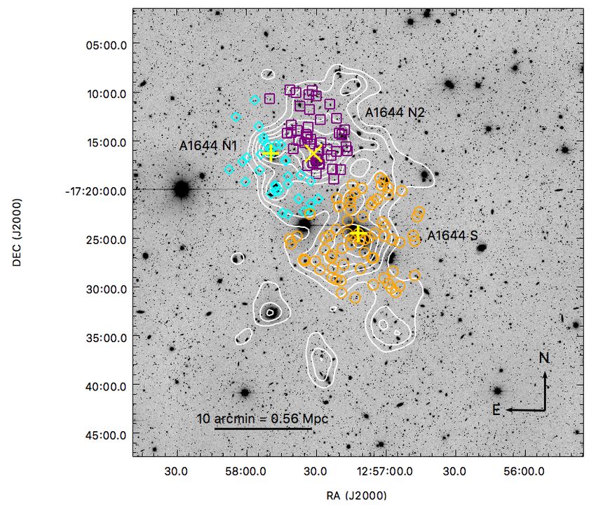
A new scenario for Abell 1644                      3

Figure 1. Optical image of the A1644 field in the r 0 band, taken with the Dark Energy Camera at Victor Blanco telescope. The red contours correspond the
Chandra X-ray image. The X-ray emission is bimodal and each peak coincides with the position of a giant elliptical galaxy (BCG S and BCG N), located at the
centre of the main (A1644S) and northern (A1644N1) structures. The new substructure found by weak lensing (Sec. 3) is labelled as A1644N2 (blue diamond).
Green and cyan dashed boxes delimit the regions used the identification of the cluster red sequence galaxies (Sec. 2). The black dashed line box encloses the
region of interest (48 arcmin2 ), which we will analyse throughout the paper.

      We used standard procedures (Valdes et al. 2014) for image re-              index lower than 0.8 and (ii.) r 0 > 19.0 with their full width at
duction/combination and astrometric calibration. The latter resulted              half-maximum (FWHM) greater than 1.3 arcsec, a value 0.2 arcsec
in a positional rms for Adelman-McCarthy (2011) catalogue stars                   above the seeing to ensure the selection of well-resolved objects.
of 0.6 ± 0.5 arcsec, which is more than enough for the purposes of
the current analysis.
                                                                                  2.2   Identification of the red sequence cluster galaxies
      Observations were made under non-photometric conditions.
This is acceptable as accurate absolute photometric calibration is                Galaxies correspond only to ∼ 5% of the total cluster mass but their
not a strong requirement for lensing, which is more concerned with                correlation in the projected space is one of the few ways to trace a
galaxy shapes and positions. In order to get an approximate cal-                  cluster in the optical band. Another useful tracer of the red cluster
ibration we used average values of the airmass extinction coeffi-                 members is their well-known correlation in the colour-colour map
cients provided by the observatory staff (Walker, private commu-                  (e.g. Medezinski et al. 2010, 2018). We identified the A1644 red-
nication), which resulted in the following zero point magnitudes:                 sequence locus on an (r 0 − i 0 ) × (g 0 − r 0 ) diagram by applying a
g0 = 31.31 ± 0.05, r0 = 31.53 ± 0.05 and i0 = 31.73 ± 0.04.                       statistical subtraction method (more details in Monteiro-Oliveira
      We used SExtractor in double image mode to create object                    et al. 2017b).
catalogues. Detections were made in the deeper r 0 image. Galaxies                      We used the galaxies within the green boxes in Fig. 1 as a
were then selected with two criteria: (i.) r 0 ≤ 19.0 CLASS_STAR                  representation of the field population and the ones inside the cyan

MNRAS 000, 1–16 (2020)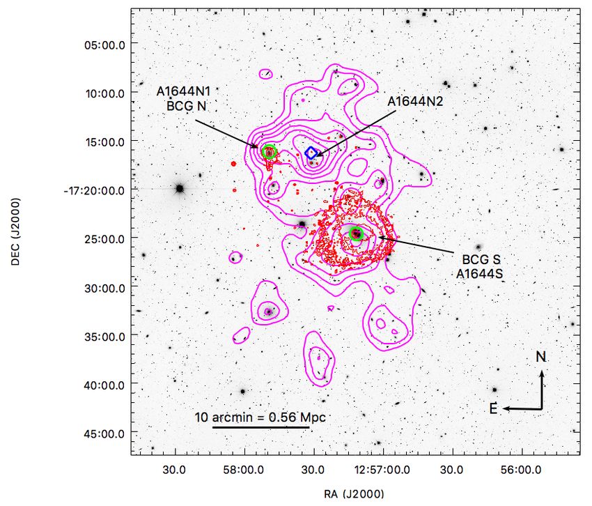
4       Monteiro-Oliveira et al.

Figure 2. Colour-colour diagram of the galaxies located at the innermost
region of the cluster field (cyan box of Fig. 1). Due to the fact that they present
homogeneous photometric properties, the red cluster member galaxies form              Figure 3. Optical image overlaid with contours of the cluster member lu-
a density peak in this space, thus defining the cluster member locus. In this         minosity map (magenta) and of the X-ray emission (red). Both BCG S and
plot, galaxies are brighter than r 0 = 19.5, considering the magnitude limit          BCG N (green circles) lie in local peaks of the luminosity map. Furthermore,
for selection of cluster members. The inset panel presents the same plot with         this shows a third relevant concentration west of A1644N1, within the Chan-
the same linear grey-scale, but for the galaxies in the control areas (green          dra field but with no visible X-ray emission. We named this substructure as
boxes in Fig. 1).                                                                     A1644N2. As we show in the text (Sec. 3.2), this galaxy concentration coin-
                                                                                      cides with the position of a dark matter clump (blue diamond). In addition,
                                                                                      we found other less significant clumps surrounding the central region. This
                                                                                      image is of the black box area defined in Fig. 1.
box as field plus cluster populations. This central region presents
a galaxy density excess in relation to the control (field) ones up to
magnitude r 0 = 19.5, which we than took as a faint limit for A1644
red-sequence galaxies. In Fig. 2 we show this density excess in the                   3.1   Source selection and shape measurement
colour-colour space. The region with the highest excess corresponds                   The background or source galaxies images constitute the raw mate-
to the locus of the A1644 early-type galaxies.                                        rial for weak lensing studies because those respond to the gravita-
     There is a total of 613 galaxies on this colour-colour locus over                tional lensing effect caused by the galaxy cluster mass. This effect
the entire optical image. We call those ‘photometric members’, yet                    manifests as a slight shape distortion on the images of the aforemen-
knowing that this sample is not free of contamination and that it                     tioned galaxies. Therefore, a careful selection of source galaxies is
does not include blue members. Their r 0 projected galaxy luminos-                    crucial for a successful weak lensing analysis.
ity distribution is presented in Fig. 3. This ‘luminosity map’ is a                         A1644 is located at a very low redshift ( z̄ = 0.047, see Sec. 4),
30 arcsec pixel-based image done by smoothing each galaxy by a                        therefore we expect most galaxies in our image to be in the clus-
bidimensional, circular Plummer profile (or an index 5 polytrope)                     ter background. In fact, for a galaxy cluster at a similar distance,
kernel with a core radius of 1 arcmin, following O’Mill et al. (2015)                 we found that foreground galaxies correspond to less than 0.2%
and Machado & Lima Neto (2015).                                                       of the CFHTLS1 catalogue (Monteiro-Oliveira et al. 2017b). This
     Although we will perform a more quantitative analysis of the                     prompted us to consider as source all galaxies fainter than r 0 = 21
red cluster galaxy luminosity peaks after the lensing analysis in                     and not in the red cluster locus on the colour-colour space (Fig. 2).
Sec. 3.2, there are obvious features in Fig. 3 that should be pointed                 Remembering that we could not detect an excess associated with
out. There X-ray maxima (A1644S and A1644N1) have their lumi-                         clusters galaxies fainter than r 0 = 19, we should have a very com-
nosity counterparts. There is one very prominent peak in the red                      plete and uncontaminated source sample.
member luminosity map with no X-ray counterpart. We label this                              To estimate the average surface critical density, that depends
substructure as A1644N2.                                                              on both the cluster and source redshifts, we applied the same cuts
                                                                                      on the CFHTLS catalogue, with photometric redshifts, and found
                                                                                      Σcr = 9.6 × 10⁹ M kpc−2 .
3   WEAK LENSING ANALYSIS                                                                   The next step is to map the point spread function (PSF), which
                                                                                      affects all image shapes across the r 0 band image used for shape
We used weak lensing techniques to recover the projected mass dis-                    measurements. To do that, we identified bright unsaturated stars
tribution on the A1644 field as estimate masses of its substructures,                 spread across the field, split them into nine frames and modelled
following the procedures we used in the study of other merging clus-                  their shapes with the Bayesian code im2shape (Bridle et al. 1998).
ters Monteiro-Oliveira et al. (2017a,b, 2018). Below we describe the                  Besides modelling individual objects as a sum of Gaussians with
data characteristics, treatment, and modelling. For a review of the
fundamentals of lensing, we refer the reader to excellent reviews
that can be found in the literature, such as Mellier (1999), Schnei-                  1 Canada-France-Hawaii Telescope Legacy Survey; http://www.cfht.
der (2005), and Meylan et al. (2006).                                                 hawaii.edu/Science/CFHTLS/

                                                                                                                                      MNRAS 000, 1–16 (2020)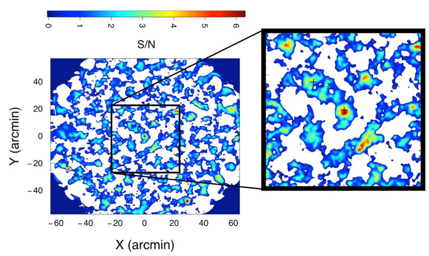
A new scenario for Abell 1644                   5
an elliptical basis, this code also deconvolves the effects of the local              Table 3. Relevant quantities for the weak lensing convergence map recon-
PSF.                                                                                  struction.
      For the PSF mapping, the star profiles are modelled as single
Gaussians and no PSF deconvolution is done. The main results of                                             Ng (gal. arcmin−2 )      10.7
this process are the ellipticity components e1 , e2 , and a size param-                                     ICF FWHM (arcmin)        2.8
eter, related to the seeing. Then, the discrete sample of parameters                                        σκ ?                    0.011
was spatially interpolated across the field with the thin plate spline
                                                                                                       ?   Noise level in the convergence map.
regression (Nychka et al. 2014) built-in R environment (R Core
Team 2014) to create a continuous function. Stellar data with dis-
crepant values were removed in 3 iterative steps; at each step, objects
                                                                                      spatially coincident with the BCG S. Also, BCG N is superposed
with the 10 per cent largest absolute residuals were discarded. The
                                                                                      with an arched clump that stretches mainly in the east-west direction.
measured stellar ellipticities and respective residuals after the spatial
                                                                                      Besides, there is some amount of significance halfway between the
interpolation are presented in Fig. 4.
                                                                                      two BCGs, whose pertinence to the targeted galaxy cluster will be
      The averaged ellipticity of all field was he1 i = 0.014 with
                                                                                      better investigated.
σe1 = 0.010 and he2 i = 0.001 with σe2 = 0.010. As stars are points
sources for all practical aspects all deviations from null values are
due to the PSF effect. As illustrated by Fig. 4, our model performed                  3.2.2   Convergence map
a good match with the data as shown by the very small averaged
residual (10−5 ) and standard deviation (0.003).                                      To create a convergence (κ) or projected mass map of the field we
      Given the PSF field at each point of the image, we used                         resorted to the maximum entropy algorithm (Seitz et al. 1998) of
im2shape over galaxies, modelling them as two Gaussians with                          the Bayesian code LensEnt2 (Marshall et al. 2002). It works by
the same elliptical base. Now the software produces PSF-free ellip-                   maximizing the evidence of the reconstructed mass field in relation
ticities and respective uncertainties. The latter are used as a quality               to the data. In order to take into account the noisiness of individual
criterion. Objects with σe > 2 or those having evidence of blending                   measurements and prevent overfitting. LensEnt2 uses a Gaussian
were removed from the source sample.                                                  intrinsic correlation function (ICF). We have tested reconstructions
                                                                                      done with a σICF ∈ [70 : 210] arcsec range.
                                                                                            For each realization of a mass map, given the ICF width, we did
3.2     The projected mass distribution                                               an automatic peak search (which is described next) and compared
3.2.1    The signal-to-noise shear map                                                the number of detected clumps above 1σ, 2σ, and 3σ. We found that
                                                                                      the number of peaks detected above 3σ remained approximately the
The ellipticities of the galaxies can be seen as noisy probes of the                  same for σICF ≥ 170 arcsec (∼ 2.8 arcmin), which we adopted as
shear field, as each galaxy has its own non-lensing related elliptic-                 bona fide. The convergence map is presented in Fig. 6 and the mass
ity. The shear field can then, through techniques, be turned into a                   reconstruction characteristics are shown in Table 3.2.2.
convergence field or a mass map. Here we created a signal-to-noise                          The S/N and the convergence maps are qualitatively very sim-
ratio (S/N) map of structures by averaging the tangential ellipticity                 ilar, both showing a wealth of structures. Some common features
e+ in relation of a grid of points, for the Nθ0 galaxies inside a radius              stand out, however; in particular, the peaks #2 and #6 of the κ map,
θ 0 , as prescribed by the mass aperture statistic (Schneider 1996),                  which are also present in the S/N map, and can be associated with
          √ Í N θ0                                                                    A1644S and A1644N1, respectively, which we already identified
            2         e+i (θ i )QNFW (θ i, θ 0 )
S/N = 2 hi=1                                  i 1/2 ,                (1)              in the member luminosity and X-ray maps. The situation is not so
          σe       N θ0                                                               clear for the remaining peaks and will be further investigated.
                                      , θ
                 Í         2
                        Q
                   i=1 NFW
                                 (θ i     0 )

where θ i is the position of the i th source galaxy and σe is the                     3.2.3   Characterization of the mass peaks
quadratic sum of the measured error and the intrinsic ellipticity
uncertainty, estimated as 0.35 for our data. We adopted the NFW                       To compute the exact position of each mass clump or peak centre,
filter (Schirmer 2004),                                                               we applied an automatic procedure. First, the algorithm searched
                                                                                      for local maxima in the convergence map within a moving circular
QNFW (θ i, θ 0 ) = [1 + e a−bχ(θi ,θ0 ) + e−c+dχ(θi ,θ0 ) ]−1 ×                       window with 2.3 arcmin radius, which allows measuring individual
                                               tanh[ χ(θ i, θ 0 )/ χc ]               peak statistics (e.g. κ̄) without any overlapping.
                                                                            ,   (2)         The peak centre position is then defined as the pixel-weighted
                                               πθ 02 [ χ(θ i, θ 0 )/ χc ]
                                                                                      mean inside the circular region. Its significance ν is the ratio between
with χ = θ i /θ 0 , which describes approximately an NFW shear                        the local maxima κmax and the noise level σκ . To measure the
profile. Hetterscheidt et al. (2005) suggest, as optimized parameters                 latter, we have performed 100 realizations of the mass distribution
for halo detection, a = 6, b = 150, c = 47, d = 50, and χc = 0.15,                    removing the cluster lens signal. This was done by rotating each
which we adopted. We also considered the radius θ 0 = 8 arcmin.                       galaxy ellipticity by a random angle [0,180[. This procedure also
The resulting S/N map can be seen in Fig. 5.                                          allowed us to identify spurious peaks caused by noise fluctuations.
      In a case like A1644, which is not a very massive cluster and                         The averaged noise level can be seen in Table 3.2.2 and a
is situated at a low redshift, that does not favour the lensing signal,               summary of the detected and expected number of spurious peaks
its structures do not stand out in the shear S/N map. In such a                       are in Table 4. As we can see, the probability to detect a spurious
case several smaller mass background structures plus line-of-sight                    peak above 4σκ is almost zero. In Table 5, we describe the most
superpositions (Yang et al. 2013; Liu & Haiman 2016) can create                       significant (ν > 4) peaks within the convergence map. Some of
similar S/N features in the map and thus the noisy appearance we                      those maybe be related to A1644 but most should be typical field
see in Fig. 5. None the less the map shows a clear high S/N clump                     features of such maps (Yang et al. 2013; Liu & Haiman 2016).

MNRAS 000, 1–16 (2020)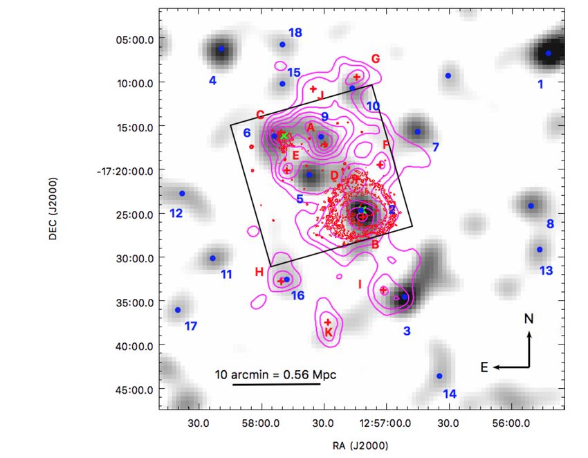
6       Monteiro-Oliveira et al.

Figure 4. PSF ellipticity. The black dots are the raw components e1 and e2 obtained from the stars and the red ones the residuals between those and the PSF
elliticity map for the 9 segments that composes a full DECam image. Dashed circles enclose 95% of the data. The averaged residuals are 10−5 for e1 and e2
with a standard deviation of 0.003 for both.

3.2.4   Correlation with cluster luminosity map                                  of 1.2 arcmin radius. We found 11 clumps (labelled A–K) with
                                                                                 significance greater than 3.5σ 2 (σ being the standard deviation
The most straightforward way to identify which of the peaks in the               of all pixels). We also computed the nearest mass clump and the
convergence map belong to A1644 is to identify possible counter-                 respective distance. These values are presented in Table 6. In Fig. 6
parts in the luminosity map. It assumes that mass and (optical) light
will follow each other, which tends to hold even for merging clusters
(Clowe et al. 2004, 2006).
      We search for peaks in the red-sequence map in a similar                   2 This slightly lower threshold was chosen so that we could find viable
manner than we did in the κ map, this time with a circular window                counterparts for all κ peaks.

                                                                                                                                MNRAS 000, 1–16 (2020)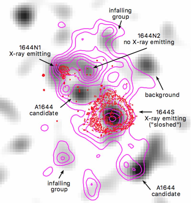
A new scenario for Abell 1644                    7

Figure 5. Signal-to-noise map obtained through the mass aperture statistic highlighting A1644 central region (Fig. 1), according to the cluster member
luminosity distribution. White regions correspond to negative S/N. The position of the two BCGs and the galaxy clump A1644N2 are marked with “+” and
“×”, respectively. The field is densely populated by mass peaks, most of them, however, due to the background large-scale structure.

Table 4. Summary of our search for mass peaks in the convergence map.         does not change significantly when we vary the smoothing scale.
                                                                              For smaller scales (5, 10 and 15 arcsec) clump A is subdivided into
                                                                              two others which became the first and second most significant. For
        Threshold interval     Number of       Expected number of
              (σκ )          detected peaks      spurious peaks               larger scales (30 and 40 arcsec), clumps A and C are merged into a
                                                                              single and most significant clump.
              [2, 3[               4                2.2 ± 2.9                       On a lower significance level, we can find two other A1644
              [3, 4[               5                0.2 ± 0.5
                                                                              substructures by associations between peaks in the red members
               ≥4                  18              0.01 ± 0.10
                                                                              luminosity and mass density maps: G-#10 offset by 78 kpc) and H-
                                                                              #16 (39 kpc). Both are on the outskirts of the A1644’s core formed
                                                                              by S, N1 and N2 substructures. They are both outside the Chandra
we show the r 0 projected galaxy luminosity distribution overlapped           image field of view.
with the projected mass map.                                                        All other galaxy concentrations are, at least, 145 kpc away
      From Fig. 6 and Table 6 we can see that A1644S and A1644N1              from the nearest mass clump, about three times more than A-#9,
are, as expected, noticeable. They are associated with the luminosity         B-#2 and C-#6, and thus their physical associations cannot be taken
peaks B (#2) and C (#6), respectively, which offset of only 42 and            for granted. E-#5 is one of such cases. It is within the core of the
49 kpc3 between luminosity and projected density peaks.                       cluster and is one of the highest peaks of the density mass map. It
      The most prominent peak in the luminosity map (A), is the               is also well inside the Chandra field of view and has no detectable
one we named A1644N2 in Sec. 2.2. It is clearly associated with               X-ray emission.
the mass density peak #9, only 51 kpc (55 arcsec) away. Due to the                  Another case is I-#3. It resembles H-#16 and G-#10 by being
absence of any detectable X-ray emission from this region on the              outside the cluster core and the X-ray image as well. The projected
Chandra image (Fig. 3), A1644N2 can be characterized as gas-poor,             distance between mass and light centres is indeed larger (146 kpc),
if not gas-free.                                                              but as it is in a much less crowded region of the field, their associa-
      Despite the absence of a dominant red galaxy, as seen in                tion seems plausible.
A1644S and A1644N1, there is a large number of galaxies in
                                                                                    In Section 4 we will use the radial velocity of cluster members
A1644N2. The significance rank of luminosity presented in Table 6
                                                                              in an attempt to solve, among other issues, the question about the
                                                                              pertinence or not of the aforementioned haloes to A1644.
3   Projected distances assuming A1644 redshift.                                    In order to check whether some of the mass map density peaks

MNRAS 000, 1–16 (2020)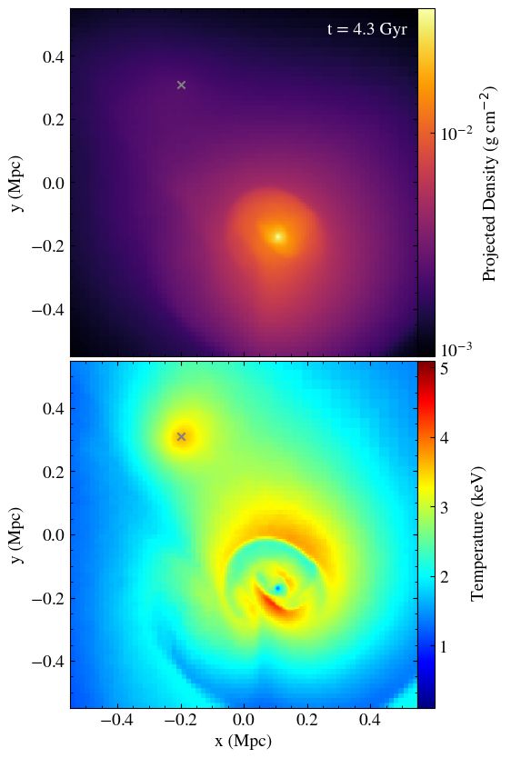
8 Monteiro-Oliveira et al.
Table 5. Statistics of the identified mass clumps. The first five columns refer to the clump ID [1], the peak centre coordinates [2–3], the peak significance
ν = κmax /σκ [4] and the mean convergence inside a circular region [5]. The mass modelled according to our model are presented in column [6] where absent
values correspond to those peaks for which our model was not able to produce reliable results (mostly because of the relatively low significance and the location
close to field border). Relevant comments on each mass clump are shown in the last column [7].
Clump α (J2000) δ (J2000) ν κ̄ (< 2.3 arcmin) M200 (1014 M ) Comments
1 12:55:42 -17:06:47 13.0 0.081 – Border/background
2 12:57:12 -17:24:47 10.6 0.071 1.90+0.89
−1.28
A1644S
3 12:56:51 -17:34:41 9.9 0.065 3.37+1.40
−2.06
A1644 candidate
4 12:58:19 -17:06:21 8.7 0.053 – Border/background
5 12:57:37 -17:20:44 8.0 0.054 0.87+0.43
−0.82
A1644 candidate
6 12:57:54 -17:16:20 7.4 0.055 0.90+0.45
−0.85
A1644N1
7 12:56:45 -17:15:48 7.2 0.048 0.81+0.40
−0.74
background
8 12:55:51 -17:24:15 6.4 0.042 – Border/background
9 12:57:31 -17:16:21 6.2 0.046 0.76+0.37
−0.75
A1644N2
10 12:57:16 -17:10:51 5.6 0.036 0.56+0.28
−0.55
A1644 candidate
11 12:58:23 -17:30:13 5.4 0.034 – Border/background
12 12:55:46 -17:29:14 4.6 0.035 – Border/background
13 12:58:38 -17:22:48 4.6 0.032 – Border/background
14 12:56:34 -17:43:40 4.4 0.033 – Border/background
15 12:57:50 -17:10:20 4.3 0.029 – background
16 12:58:40 -17:36:10 4.2 0.034 – A1644 candidate
17 12:57:48 -17:32:42 4.2 0.029 – Border/background
18 12:57:50 -17:05:52 4.1 0.028 – Border/background
would be associated with some massive background structure, we component g+ by the lensing convolution kernel,
looked for associations between them and overdensities in the back-
y2 − x2 −2x y
ground galaxy sample. We failed to find any. Our interpretation is, D1 = 2 , D2 = 2 , (3)
therefore, that most of the κ peaks not associated with A1644 should x + y2 x + y2
be due to constellations of (. 1013 M ) background haloes which where x and y are the Cartesian coordinates relative to the lens
dominate the population of low peaks in the field (e.g. Yang et al. centre which was considered at the respective mass peak position.
2013; Liu & Haiman 2016; Wei et al. 2018). The resulting reduced shear that will affect the image of each
source galaxy can be written as
NÕ
clumps
gi = gik , (4)
3.3 Mass estimation k=1
with i ∈ {1, 2}. As we modelled the mass peaks in the region of
3.3.1 Mass field modelling
interest, Nclumps = 18.
The weak lensing masses of the individual mass clumps are in The model adopted is as a single circular NFW profile per
general better recovered by fitting physically motivated profiles. In clump or halo (Navarro et al. 1996, 1997). The χ2 -statistic is then
crowded fields, such as the one we are dealing with, it can be done
NÕ
individually as there will be clear covariances between the several
2
sources Õ
[gi (M200, c) − ei, j ]2
χ2 = , (5)
substructures. Here we will fit simultaneously 18 structures, which
j=1 i=1 σint
2 + σ2
obs
we will treat as dark matter haloes centred on the peaks with ν > 4 i, j
found in the κ map. where gi (M200, c) is the reduced shear (Eq. 4) produced by all the
The weak gravitational lensing effect induced on each source NFW haloes over the position of a given source galaxy, M200 is the
galaxy is a combination of those generated by each of the individual mass within a radius where the mean enclosed density is equal to
mass clumps. Here, we will adopt a simplified model in which all of 200× the critical density of the Universe, c is the halo concentration
them are located at the same cluster redshift. It is easier, in this case, parameter, ei, j is the measured ellipticity parameter per galaxy,
to deal with the Cartesian components of the reduced shear, g1 and σobsi, j is its measurement uncertainty and σint is the shape noise,
g2 , which are obtained by projecting the lens generated tangential taken as ∼ 0.35 for our data.
MNRAS 000, 1–16 (2020)A new scenario for Abell 1644 9
Figure 6. Mass-luminosity correlation. Projected mass map (grey-scale) overlaid with the luminosity density distribution of red cluster members (magenta
contours). Blue dots mark the mass peak centres (labelled 1–18) whereas the red “+” are placed at the galaxy clumps centre (A–H). BCGs positions are marked
with green “×” symbols. The black box shows the X-ray Chandra image field of view.
The likelihood can now be written as 3.3.2 Model assessment
χ2 Before stating the results, given the complexity of this field, mostly
ln L ∝ − . (6)
2 driven by the low signal from the very nearby cluster, we felt the need
There are 2 × Nclumps free parameters in our model which can to further ensure the reliability of the whole modelling procedure.
lead to instabilities in the final model. We thus opt to reduce this We created a synthetic reduced shear field by positioning NFW
number in half by adopting the M200 − c relation by Duffy et al. lenses at the same position of the eighteen detected mass density
(2008): peaks plus a population of source galaxies also at the same position
as the ones in our background sample.
−0.084
M200 For this model, we got the mass of A1644S from the X-ray
c = 5.71 (1 + z)−0.47 . (7) mass by Johnson et al. (2010)4 . The remaining masses were set by
2 × 10¹² h−1 M
multiplying this value to the ratio of the peak heights (ν/ν A1644S ;
Given that the above relation having a scatter, we opt to not include Table 5). The reduced shear components for each galaxy were then
it in our model in order to keep the parameter space to a minimum, set as the sum of the contributions of each of the lenses. We did not
given the complexity of the field. add anything else to take into account the shape or measurement
Finally, the posterior can be written as noises.
Pr(M200 |data) ∝ L(data|M200 ) × P(M200 ), (8)
where we adopted an uniform prior P(M200 ), 0 < M200 ≤ 8 × 10¹⁵ 4 The value was converted from M500 to M200 = 4.65×10¹⁴ M (following
M . an NFW profile) to be used here.
MNRAS 000, 1–16 (2020)10 Monteiro-Oliveira et al.
Table 6. Characteristics of the peaks found in the luminosity map of red- of the model assumptions with the real clumps, for example, the
sequence galaxies. Columns are, respectively: ID, position, significance in absence of axisymmetry and/or a deviation from the theoretical
units of σ (standard deviation of all pixels), the nearest mass peak ID and profile.
the respective projected distance assuming A1644 redshift. The haloes directly related to the X-ray emission, A1644S
(#2) and A1644N1 (#6), have masses of 1.90+0.89 −1.28
× 1014 M
+0.45 14
and 0.90−0.85 × 10 M , respectively. Both are considerably
Clump α δ S Nearest Distance
smaller than X-ray measurements presented by Johnson et al. (2010)
ID (J2000) (J2000) (σ) mass clump (kpc)
(A1644S: 4.6 ± 0.6; A1644N1: 3.8 ± 0.6). The discrepancy is no-
A 12:57:30 -17:17:12 5.8 #9 51 ticeable but not a total surprise as the A1644 ICM is out of hy-
B 12:57:11 -17:25:32 5.0 #2 42 drodynamical equilibrium and this surely affects the X-ray mass
estimation.
C 12:57:50 -17:15:51 4.9 #6 49 As for A1644N2 (#9) we got M200 = 0.76+0.37 −0.75
× 1014 M .
D 12:57:14 -17:21:12 4.4 #2 201 Therefore, the core of A1644 has a combined mass of 3.99+1.39−1.59
×
E 12:57:48 -17:20:11 4.2 #5 145 1014 M , corresponding to the sum of the S+N1+N2 posteriors.
F 12:57:03 -17:19:32 4.1 #7 314 Adding the candidate clump #5, the value increases to 5.11+1.32
−1.44
×
1014 M .
G 12:57:14 -17:09:32 3.8 #10 78
Substructure #3 came out of the analysis as the single most
H 12:57:51 -17:32:51 3.6 #16 39 massive clump of the field, although with rather large error bars:
I 12:57:02 -17:33:52 3.6 #3 146 3.37+1.40
−2.06
× 1014 M . It was rather unexpected, given that its con-
vergence peak is almost the same height as #2 (A1644S), whose
J 12:57:35 -17:10:52 3.5 #15 195
nominal mass value is almost half of it. Also there are not so many
K 12:57:28 -17:37:32 3.5 #16 372 cluster galaxies associated with it, assuming a I-#3 connection, nor
any hints of a background structure in the photometry data. From
the κ map (Fig. 6) it seems that it may have an extension or (pro-
jected) neighbours to the NW direction, which might enhance its
Given the high degree of idealisation idealization of this sim-
mass somewhat.
ulation, one should expect all the results to be very close to the true
Regarding the A1644 candidate structures, our model was not
ones, and it happens for those with higher peak heights and on the
able to recover the mass of #16. The masses of #5 and #10 are
0.87+0.43 × 10¹⁴ and 0.56+0.28
core of the cluster.
−0.82 −0.55
× 1014 M , respectively.
However, in some cases, the recovered representative mass
value5 was considerably larger than the reference (> 35%). We
mention, as an example, the case of clump #14 whose measured
mass was 56% larger than stated in the synthetic catalogue. These 4 DYNAMICAL ANALYSIS
mass clumps have in common: (i) their relative low significance ν From the radial velocities available in the literature we explore the
and/or (ii) their proximity to the border of the region considered for complex dynamical picture of A1644. We are particularly inter-
modelling. Based on these arguments, we decided not to consider ested in verifying whether the mass substructures found through
the MCMC results for the clumps with ν < 5.5, nor those located our photometric plus weak lensing analysis are actually dynamical
close to the borders. structures bound to the main cluster.
3.3.3 Results 4.1 Identification of the spectroscopic cluster members
We restricted the source galaxies used in the model to those con- The field of A1644 has been exhaustively observed by the WIde-
tained in the central region of interest (Fig. 1). Then, we sampled field Nearby Galaxy-cluster Survey (WINGS; Fasano et al. 2006).
the posterior (Eq. 8) using the MCMC algorithm with a simple As a result, a simple search on the NASA Extragalactic Database
Metropolis sampler MCMCmetrop1R (Martin et al. 2011) built in (NED)6 has revealed a total of 360 galaxies with available redshifts
R environment. We generated four chains with 105 iterations each located inside a circular region of 33 arcmin centred on A1644S.
one, removing the first 104 as “burn-in”. The final convergence, After searching on our galaxy catalogue, we have found photometric
checked through the potential scale factor R implemented in the counterparts for 341 objects whose redshift distribution can be seen
Coda library (Plummer et al. 2006), is attested within 68 per cent in Fig. 7.
c.l. (R ≈ 1). A simple approach to select the cluster spectroscopic members
The results, median of the marginalized values of M200 , can consists of the application of the 3-σ clipping method (Yahil &
be seen in Table 5. All the posteriors are unimodal, although not Vidal 1977). Despite its simplicity, this procedure is sufficiently
symmetrical (and hence the difference in the plus and minus uncer- accurate to remove the most obvious outliers of the sample (Wojtak
tainties) and not degenerate. The higher correlations are still small – et al. 2007). The resulting sample consisted of 249 galaxies with
namely between the masses of A1644S and #5 (-0.25) and A1644S z̄ = 0.0471 ± 0.0002 and σv /(1 + z̄) = 1017 km s−17 (hatched
and #3 (-0.21). region in Fig. 7). According to the Anderson-Darling test, the null
As we can observe in Table 5 the ratio of fitted mass to mass
uncertainty is smaller than the detection (e.g. Martinet et al. 2016).
6 https://ned.ipac.caltech.edu/
One possible mechanism responsible for that is the non-conformity
7 The (1 + z)−1 factors that appears multiplying velocity dispersions or
differences are there to compensate for the cosmological stretching of ve-
5 Corresponding to the median of each marginalized posterior. locities.
MNRAS 000, 1–16 (2020)A new scenario for Abell 1644 11
of the galaxies in substructures are spatially coincident with the
mass clumps G-#10 and H-#16, previously identified as subcluster
candidates. Thus, their high dynamical deviation with respect to the
other members strongly suggest that both belong to a non-virialised
regions being most probably infalling groups (Einasto et al. 2018).
4.2 Identifying the subclusters with Mclust
The R-based package Mclust (Chris Fraley & Scrucca 2012) en-
compasses functions designed to perform multidimensional normal
mixture modelling based on the analysis of finite mixture of distri-
butions. It works by searching for the optimized clustering of the
data using models with variable shape, orientation and volume. A
prior restricting the number of normal components is allowed. The
output includes number and characteristics of the components plus
the individual memberships. More details about the use of Mclust
to search for substructures in the observable phase space of a cluster
can be found in Einasto et al. (2012).
Figure 7. Redshift distribution in A1644 region. We have selected the spec- At this point we already established that A1644 is composed
troscopic cluster members after a 3σ-clipping procedure. The selected mem-
of several substructures, probably in merger, but its 1D velocity
bers are highlighted by hashing lines and are shown in more detail in the
upper right panel. The 249 selected members have z̄ = 0.0471 ± 0.0002
distribution is very consistent with normalcy. It is a hint that the
with σv /(1 + z) = 1017 km s−1 . subclusters’ motions are taking place almost parallel to the plane of
the sky (e.g. Monteiro-Oliveira et al. 2018; Wittman et al. 2018a).
As a consequence, one-dimensional methods, i.e. those based only
on the radial velocity information, will certainly fail to assign con-
hypothesis of Gaussianity cannot be discarded for this sample within
fidently the galaxies to a host subcluster. In fact, as a confirmation,
a confidence level of 95% (p − value = 0.21). This is in agreement
1D-Mclust pointed out that the single-component model is strongly
with recent findings of Lopes et al. (2018).
favoured in relation to a bimodal distribution in the redshift space
Although the overall distribution of redshifts is Gaussian it
as revealed by Bayesian information criteria (Kass & Raftery 1995)
does not necessarily mean that there are no substructures present.
as ∆BIC = 16.
To search for those, we have applied the well-known ∆-test (Dressler
Given this scenario, we directed our efforts to the analysis of
& Shectman 1988), that looks for structures in both velocity space
the spatial distribution of cluster members within the cluster core.
and projected position, and are described by the following equations:
The sample used here consists of the projected position (α and δ) of
combined photometric red-sequence and spectroscopic members.
Nnb + 1
1/2
Since this data is spread across all the field, we have restricted our
δi = [(v̄l − v̄) 2
+ (σl − σ) 2
] (9)
σ2 region of interest to the inner part, selecting only the galaxies inside
two circular regions, each one with a radius of 7 arcmin, centred on
N
the BCG S and on the mid-point between A1644N1 and A1644N2.
Õ
∆= δi . (10) See Fig. 9 for the positions of the 163 galaxies of this sample.
i=1
The application of 2D-Mclust showed the data are best de-
scribed as a bimodal distribution. This model is strongly favoured
For a cluster hosting any substructures, Dressler & Shectman (1988) with respect to the second-best model with three groups, as pointed
suggest ∆ ≥ N as the expected statistics. However, Hou et al. (2012) out by ∆BIC = 12. In both scenarios the two main groups contain
have proposed an improved index based on the p − value < 0.01 most of the sample. In the case with three groups, the third one has a
to identify a substructure (see Monteiro-Oliveira et al. 2017a, for a few galaxies on the SE direction of A1644S (or clump B-#1; Fig. 6).
more complete description of this statistic). The outcome is a cut in the sample along the SE–NW direction, sep-
The application of the ∆-test in our sample returned ∆ = 339 arating A1644S at one side and A1644N1/N2 at the other (orange
with a p-value of 0.007, both pointing to the presence of substruc- points versus cyan and purple on Fig. 9). This division is consistent
tures. The spatial distribution of the spectroscopic members overlaid with the position of the most significant galaxy clumps according
with the ∆-test results is shown as a “bubble plot” (Fig. 8). to Table 6. We also performed the exercise to include the redshift
The ∆-test does not identify which individual galaxies belong information9 for a tri-dimensional analysis with 3D-Mclust. The
to a substructure. In Monteiro-Oliveira et al. (2017a), however, result was a return to unimodality.
we envisaged a process to do so by searching for a threshold δc In order to understand the dynamical process that formed the
(equation 9). All galaxies having δi ≥ δc 8 were therefore considered complex A1644 as we see today, we are interested in estimating the
part of some substructure and then excluded of the main sample relative velocities between the clumps we found both by photometry
(galaxies marked with “×” in Fig. 8). and weak lensing. In order to do that, we reran 2D-Mclust over the
We ended up with 210 galaxies in the main sample with similar northern sample it already identified and imposed a division in two
average and dispersion than the original 249 members sample. Most groups. These results are presented in Fig. 9 (cyan versus purple
8 We have adopted δ c = 2 which has been shown to be a good threshold to
remove the substructures. 9 For those galaxies for which this information is available.
MNRAS 000, 1–16 (2020)12 Monteiro-Oliveira et al.
Figure 8. Bubble plot produced with ∆-test results. The filled circles indicate each galaxy position and their radius are proportional to e δ i meaning that the
larger this value, the more relevant the substructure is. To make their positions clear, two “+” signals are placed at the BCGs locations. The mass clump IDs
are placed at the exact place of the corresponding centre. The colour bar represents the peculiar velocities vi − v̄ and “×” indicates the galaxies classified as
belonging to some substructure according to our δi ≥ 2 criterion. Our final sample consisted of 210 galaxies characterized by the same mean redshift and
velocity dispersion of the initial sample. Note that this region is somewhat larger than those defined in Fig. 1.
points) and now we have clear samples that can be associated with only. In the simulation presented here, A1644N1 is not included.
each of the three main core structures (S, N1, and N2). For a more detailed analysis of the set of simulations, the reader
In Table 7, we show redshifts and velocity dispersions from is referred to an accompanying paper (Doubrawa et al. 2020), in
the redshifts we have for each of those samples. In Table 8, we show which we explore the outcomes of alternative scenarios and discuss
the differences in (rest-frame) velocities. As expected we find small their relative advantages and disadvantages. In this section, we will
separations between them, in the velocity space, not inconsistent describe the main features of one plausible model.
with zero given the uncertainties. To have an acceptable scenario, some constraints must be sat-
isfied by the simulations: the virial masses and virial radii estimated
in this paper; the spiral morphology of cold gas, with an extent of ap-
proximately 200 kpc; the observed projected separation of ∼550 kpc
5 HYDRODYNAMICAL SIMULATIONS
between the structures; and simultaneously A1644N2 must have a
In this section, we employ N-body hydrodynamical simulations to low fraction of gas to be nearly undetectable in X-ray observations.
evaluate whether the newly discovered structure A1644N2 could be Taking the new virial mass estimates, 1.9 × 10¹⁴ M for
responsible for the collision that gave rise to the sloshing spiral. A1644S and 0.76×10¹⁴ M for A1644N2, we create two spherically
Several simulations were performed in search of a model that repro- symmetric galaxy clusters that are initially in hydrostatic equilib-
duces some of the desired morphological features of A1644. Here rium. The method for generating initial conditions is similar to those
we present one model that successfully recovers the spiral morphol- used in Machado & Lima Neto (2015). Each cluster is created with
ogy of A1644S: it is an encounter between A1644S and A1644N2 2 × 10⁶ particles, divided equally between gas and dark matter, fol-
MNRAS 000, 1–16 (2020)A new scenario for Abell 1644 13
Table 7. Statistics of galaxy groups found with 2D-Mclust.
A1644S A1644N1 A1644N2
Number of galaxies 42 17 17
z̄ 0.0472 ± 0.0006 0.0476 ± 0.0007 0.0460 ± 0.0012
σv /(1 + z̄) ( km s−1 ) 1146+211
−59
886+261
−85
1376+402
−134
adequate shape and extent. Fig. 10 shows the projected density,
and the emission-weighted temperature map of the hydrodynamical
simulation at t = 4.3 Gyr, highlighting the presence of A1644N2
with the symbol ×.
After the first pericentric passage, A1644N2 loses almost all
of its gas, making it difficult to identify in X-ray observations. It
retains about 0.1−1 per cent of its initial gas mass. In order to obtain
a projected separation of approximately 550 kpc between clusters,
at the best match of morphology, the orbital plane was inclined by
i ≈ 30◦ with respect to the plane of the sky. This is compatible with
the low line-of-sight velocity found by the observational analysis
(Table 8). We can estimate this relative velocity between A1644S
and A1644N2 through the displacement between the clusters cores
in the z-axis inside a short time step around t = 4.3 Gyr. This
approach results in a line-of-sight velocity of ∼ 100 km s−1 , in
agreement with the low values expected in a merging system near
their maximum separation.
Our goal was to recover the morphological features observed in
A1644 through hydrodynamical simulations. To judge the adequacy
of the simulation results, most comparisons were made by qualita-
Figure 9. Galaxy classification suggested by double application of 2D- tive visual inspection of the morphology. The model presented is
Mclust. The picture shows the spatial distribution of the members of one of the possible combinations of the collision parameters. With
A1644S (orange), A1644N1 (cyan), and A1644N2 (purple) overlaid with this scenario, we were able to reproduce, in a best instant, several
the numerical density contours of the combined sample containing both of the simulation constraints, such as morphology, temperature and
spectroscopic and photometric members (white lines). For comparison, “+” extent of the sloshed gas, projected separation and low X-ray emis-
are placed at BCGs positions and “×” marks the position of the mass clump sion of A1644N2, with the virial masses and radii derived from the
A1644N2.
gravitational weak lensing analysis. Our current plausible model
is thus the scenario in which A1644N2 is the disturber that in-
duced the sloshing. Other scenarios involving A1644N1 instead of
Table 8. Dynamics of the subclusters A1644S, A1644N1, and A1644N2 A1644N2 did not give rise to results as satisfactory as the model
modelled by 2D-Mclust. Projected distances were computed based on the presented here. Alternative simulations are explored in more detail
respective mass peak positions. All error bars correspond to 68 per cent c.l. in Doubrawa et al. (2020).
Pairs δv/(1 + z̄) (km s−1 ) Projected distance (kpc)
S–N1 137 ± 278 723 6 DISCUSSION
S–N2 334 ± 378 531
N1–N2 471 ± 397 298 We presented here a comprehensive analysis of the nearby merg-
ing galaxy cluster Abell 1644. With a combination of observational
and computational techniques, we were able to propose a new de-
scription for the preceding collision events which led to the current
lowing the procedure described in Machado & Lima Neto (2013). state. We put forth a scenario in which the remarkable spiral-like
Simulations were carried out with Gadget-2 (Springel 2005). Ini- structure seen in the X-ray emission of A1644S arose as a result of
tially the clusters are separated by 3 Mpc along the x-axis, with the interaction with the newly discovered subcluster A1644N2 and
an impact parameter of b = 800 kpc, and initial relative velocity not due to A1644N1 as suggested by previous studies.
of −700 km s−1 in the x direction (at t = 0). The evolution of the From large field-of-view images taken in three broad-bands,
system is followed by 5 Gyr. we built a careful selection of the galaxy samples. The luminosity
The desired configuration is achieved at t = 4.3 Gyr, that is, map of the red cluster sequence galaxies (Fig. 3) brought the first
1.6 Gyr after the pericentric passage and 0.5 Gyr after reaching the hint that the cluster morphology should be somewhat more com-
maximum separation of 770 kpc. This model presents temperature plex than previously claimed. Besides the two prominent galaxy
maps that are in good qualitative agreement with the expected ranges clumps related to each BCG (A1644S and A1644N1), a third one,
presented in Reiprich et al. (2004b) and Johnson et al. (2010). not reported in previous studies, was found slightly to the West
Similarly, the spiral morphology of cool gas in A1644S displays of BGC N (A1644N2). Surrounding these central concentrations,
MNRAS 000, 1–16 (2020)14 Monteiro-Oliveira et al.
Figure 11. Proposed scenario for the merging cluster A1644. The weak
lensing mass map (gray-scale) is overlaid with the r 0 projected galaxy lumi-
nosity distribution (magenta contours) and X-ray emission (red contours).
The main subcluster, A1644S has a spiral-like pattern in its ICM distribution
caused by the passage the gas-poor subcluster A1644N2, found in this work.
The cluster core is also formed by the X-ray emitting subcluster A1644N1.
There are also two infalling galaxy groups in the cluster vicinity. We clas-
sified as A1644 candidates two significant mass clumps surrounded by red
galaxies.
Figure 10. Top panel: Projected density map for the merger simulation
between A1644S and A1644N2, at t = 4.3 Gyr. Bottom panel: Pro- ing mass maps (Dietrich et al. 2012). The three main structures are
jected emission-weighted temperature. The symbol marks the presence of separated from each other by 723 kpc (S–N1), 531 kpc (S–N2), and
A1644N2, nearly undetectable on the density map. 298 kpc (N1–N2). The total mass content of A1644 is evaluated in,
at least, M200 = 3.99+1.39
−1.59
× 1014 M .
From the catalogue of radial velocities available in the litera-
two others can be found in the cluster outskirts. Further analysis ture, we were able to provide some insights about the dynamics of
based on their radial velocities, showed that they consist of infalling A1644. Regarding the three main subclusters, we found that they are
groups. There are also two galaxy clumps located reasonably close not so apart in relation to the line of sight, having δv/(1 + z̄) < 470
to significant mass concentrations, but with no spatial coincidence. km s−1 (Table 8) and, within the uncertainties, compatible with a
With our analysis, we cannot categorically state if they are part of negligible separation (e.g. Wittman et al. 2018a).
the cluster, though it could be possible. Conservatively, we clas- One probe of the perturbed state of a system is how its veloc-
sified both as A1644 candidates. However, for the description of ity dispersion was boosted during the merger process (e.g. Pinkney
the merger process among the main subclusters, the presence of et al. 1996; Takizawa et al. 2010; Monteiro-Oliveira et al. 2018). For
such structures can be disregarded as a first approximation. These an idealized isolated system, the pre-merger velocity dispersion σpre
findings are illustrated in Fig.11. can be estimated from an empirical relation M200 –σv (e.g. Biviano
In this work, we presented the first weak-gravitational lensing et al. 2006). To do this, we considered the entire sample of 4 × 10⁵
recovered projected mass distribution of the extremely low-z merg- mass values from the MCMC mass modelling (Sec. 3.3.3). We found
ing cluster Abell 1644. Since this technique does not assume any 656+146
−109
km s−1 for A1644S, 528+135 −107
km s−1 for A1644N1 and
+132 −1
502−101 km s for A1644N2. After the pericentric passage, the ve-
prior about the dynamical state, it is a powerful tool to recover the
total mass of cluster haloes. The projected mass map corroborates locity dispersion σobs is easily obtained (see Table 7). Therefore, the
the scenario indicated by the projected galaxy luminosity distribu- boost factors f ≡ σobs /σpre , are fS = 1.8+0.4 , f = 1.7+0.6
−0.6 N1 −0.7
and
tion, with each of the three main galaxy concentrations related to +0.9
fN2 = 2.8−1.2 , respectively for A1644S, A1644N1 and A1644N2.
a respective mass clump. In A1644S, the BCG matches exactly the The amount of events where the final velocity dispersion was not
mass clump centre whereas A1644N1 is displaced only 56 kpc in greater than unity (i.e. σpre was not enhanced by the collision) was
relation to that. However, projected separations up to ∼ 100 kpc 2 per cent, 10 per cent and 2 per cent for A1644S, A1644N1, and
are not statistically significant because is also comparable with the A1644N2, respectively. However, these results should be consid-
expected effect caused by shape noise and smoothing of weak lens- ered with parsimony since velocity dispersion, specially from the
MNRAS 000, 1–16 (2020)You can also read