RGB-D image-based Object Detection: from Traditional Methods to Deep Learning Techniques
←
→
Page content transcription
If your browser does not render page correctly, please read the page content below
Chapter 3
                                         RGB-D image-based Object Detection: from
                                         Traditional Methods to Deep Learning
                                         Techniques

                                         RGB-D Image Analysis and Processing
arXiv:1907.09236v1 [cs.CV] 22 Jul 2019

                                         Isaac Ronald Ward, Hamid Laga, and Mohammed Bennamoun

                                         Abstract Object detection from RGB images is a long-standing problem in image
                                         processing and computer vision. It has applications in various domains including
                                         robotics, surveillance, human-computer interaction, and medical diagnosis. With
                                         the availability of low cost 3D scanners, a large number of RGB-D object detection
                                         approaches have been proposed in the past years. This chapter provides a compre-
                                         hensive survey of the recent developments in this field. We structure the chapter into
                                         two parts; the focus of the first part is on techniques that are based on hand-crafted
                                         features combined with machine learning algorithms. The focus of the second part is
                                         on the more recent work, which is based on deep learning. Deep learning techniques,
                                         coupled with the availability of large training datasets, have now revolutionized the
                                         field of computer vision, including RGB-D object detection, achieving an unprece-
                                         dented level of performance. We survey the key contributions, summarize the most
                                         commonly used pipelines, discuss their benefits and limitations, and highlight some
                                         important directions for future research.

                                         3.1 Introduction

                                         Humans are able to efficiently and effortlessly detect objects, estimate their sizes and
                                         orientations in the 3D space, and recognize their classes. This capability has long
                                         been studied by cognitive scientists. It has, over the past two decades, attracted a lot
                                         of interest from the computer vision and machine learning communities mainly be-

                                         Isaac Ronald Ward
                                         University of Western Australia, e-mail: isaac.ward@uwa.edu.au
                                         Hamid Laga
                                         Murdoch University, Australia, and The Phenomics and Bioinformatics Research Centre, Univer-
                                         sity of South Australia, e-mail: H.Laga@murdoch.edu.au
                                         Mohammed Bennamoun
                                         University of Western Australia, e-mail: mohammed.bennamoun@uwa.edu.au

                                                                                                                                   1
2                              Isaac Ronald Ward, Hamid Laga, and Mohammed Bennamoun

cause of the wide range of applications that can benefit from it. For instance, robots,
autonomous vehicles, and surveillance and security systems rely on accurate de-
tection of 3D objects to enable efficient object recognition, grasping, manipulation,
obstacle avoidance, scene understanding, and accurate navigation.
    Traditionally, object detection algorithms operate on images captured with RGB
cameras. However, in the recent years, we have seen the emergence of low-cost 3D
sensors, hereinafter referred to as RGB-D sensors, that are able to capture depth
information in addition to RGB images. Consequently, numerous approaches for
object detection from RGB-D images have been proposed. Some of these methods
have been specifically designed to detect specific types of objects, e.g. humans, faces
and cars. Others are more generic and aim to detect objects that may belong to one
of many different classes. This chapter, which focuses on generic object detection
from RGB-D images, provides a comprehensive survey of the recent developments
in this field. We will first review the traditional methods, which are mainly based
on hand-crafted features combined with machine learning techniques. In the second
part of the chapter, we will focus on the more recent developments, which are mainly
based on deep learning.
    The chapter is organized as follows; Section 3.2 formalizes the object detection
problem, discusses the main challenges, and outlines a taxonomy of the different
types of algorithms. Section 3.3 reviews the traditional methods, which are based on
hand-crafted features and traditional machine learning techniques. Section 3.4 fo-
cuses on approaches that use deep learning techniques. Section 3.5 discusses some
RGB-D-based object detection pipelines and compares their performances on pub-
licly available datasets, using well-defined performance evaluation metrics. Finally,
Section 3.6 summarizes the main findings of this survey and discusses some poten-
tial challenges for future research.

3.2 Problem statement, challenges, and taxonomy

Object detection from RGB-D images can be formulated as follows; given an
RGB-D image, we seek to find the location, size, and orientation of objects of in-
terest, e.g. cars, humans, and chairs. The position and orientation of an object is
collectively referred to as the pose, where the orientation is provided in the form of
Euler angles, quaternion coefficients or some similar encoding. The location can be
in the form of a 3D bounding box around the visible and/or non-visible parts of each
instance of the objects of interest. It can also be an accurate 2D/3D segmentation,
i.e. the complete shape and orientation even if only part of the instance is visible.
In general, we are more interested in detecting the whole objects, even if parts of
them are not visible due to clutter, self-occlusions, and occlusion with other objects.
This is referred to as amodal object detection. In this section, we discuss the most
important challenges in this field (Section 3.2.1) and then lay down a taxonomy for
the state-of-the-art (Section 3.2.2).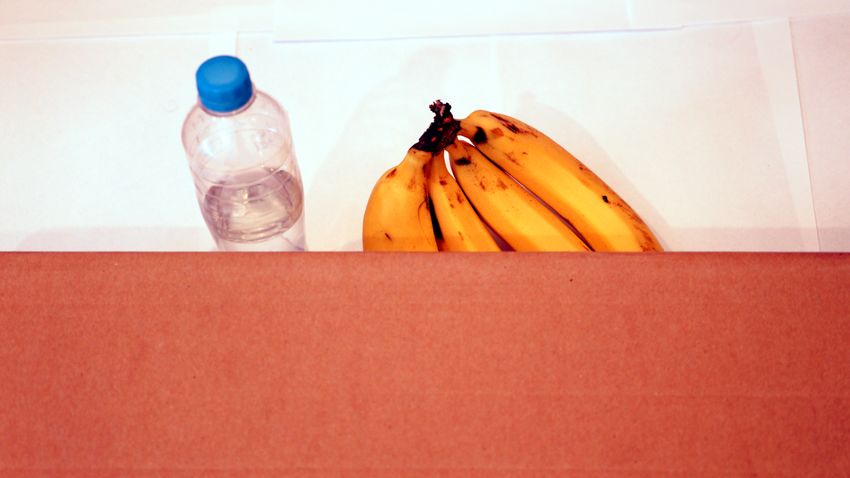
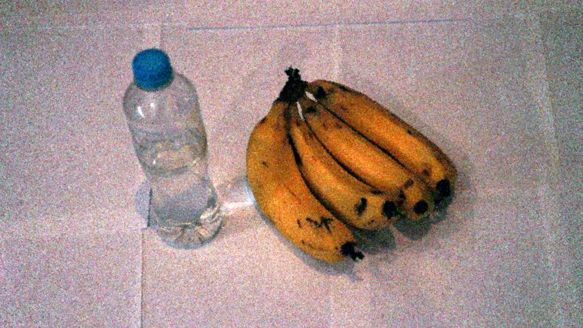
3 A Survey on RGB-D image-based Object Detection                                       3

  (a)                           (b)                           (c)

  (d)                           (e)                           (f)

Fig. 3.1: Illustration of some extrinsic challenges in object detection. (a) Objects of
interest are clearly separated from each other and from the uniform background. (b)
Two objects partially occluded by a cardboard box. (c) Sensor noise that might affect
images. (d) An overexposed image. (e) An underexposed image. (f) A cluttered
image, which hinders the detection of smaller and occluded objects.

3.2.1 Challenges

Though RGB-D object detection has been extensively investigated, there are a num-
ber of challenges that efficient solutions should address. Below, we classify these
challenges into whether they are due to intrinsic or extrinsic factors. Extrinsic fac-
tors refer to all the external factors that might affect object detection (see Fig. 3.1).
Extrinsic challenges include:
• Occlusions and background clutter. The task of object detection algorithms is
  to not only localize objects in the 3D world, but also to estimate their physical
  sizes and poses, even if only parts of them are visible in the RGB-D image.
  In real-life situations, such occlusions can occur at anytime, especially when
  dealing with dynamic scenes. Clutter can occur in the case of indoor and outdoor
  scenes. While biological vision systems excel at detecting objects under such
  challenging situations, occlusions and background clutter can significantly affect
  object detection algorithms.
• Incomplete and sparse data. Data generated by RGB-D sensors can be incom-
  plete and even sparse in some regions, especially along the z−, i.e. depth, direc-
  tion. Efficient algorithms should be able to detect the full extent of the object(s)
  of interest even when significant parts of it are missing.
• Illumination. RGB-D object detection pipelines should be robust to changes in
  lighting conditions. In fact, significant variations in lighting can be encountered
  in indoor and outdoor environments. For example, autonomously driving drones
  and domestic indoor robots are required to operate over a full day-night cycle
  and are likely to encounter extremes in environmental illumination. As such, the
  appearance of objects can be significantly affected not only in the RGB image

4                              Isaac Ronald Ward, Hamid Laga, and Mohammed Bennamoun

    (a)                        (b)                           (c)

    (d)                        (e)                           (f)

Fig. 3.2: Illustration of some intrinsic challenges in object detection. (a-c) Intra-
class variations where objects of the same class (chair) appear significantly different.
(d-f) Inter-class similarities where objects belonging to different classes (cat, cougar
& lion) appear similar.

  but also in the depth map, depending on the type of 3D sensors used for the
  acquisition.
• Sensor limitations. Though sensor limitations classically refer to colour image
  noise that occurs on imaging sensors, RGB-D images are also prone to other
  unique sensor limitations. Examples include spatial and depth resolution. The
  latter limits the size of the objects that can be detected. Depth sensor range limi-
  tations are particularly noticeable, e.g. the Microsoft Kinect, which is only suffi-
  ciently accurate to a range of approximately 4.5m [79]. This prevents the sensor
  from adequately providing RGB-D inputs in outdoor contexts where more ex-
  pensive devices, e.g. laser scanners, may have to be used [56].
• Computation time. Many applications, e.g. autonomous driving, require real-
  time object detection. Despite hardware acceleration, using GPUs, RGB-D-based
  detection algorithms can be slower when compared to their 2D counterparts. In
  fact, adding an extra spatial dimension increases, relatively, the size of the data.
  As such, techniques such as sliding windows and convolution operations, which
  are very efficient on RGB images, become significantly more expensive in terms
  of computation time and memory storage.
• Training data. Despite the wide-spread use of RGB-D sensors, obtaining large
  labelled RGB-D datasets to train detection algorithms is more challenging when
  compared to obtaining purely RGB datasets. This is due to the price and com-
  plexity of RGB-D sensors. Although low cost sensors are currently available, e.g.
  the Microsoft Kinect, these are usually more efficient in indoor setups. As such,
  we witnessed a large proliferation of indoor datasets, whereas outdoor datasets
  are fewer and typically smaller in size.
3 A Survey on RGB-D image-based Object Detection                                      5

Intrinsic factors, on the other hand, refer to factors such as deformations, intra-class
variations, and inter-class similarities, which are properties of the objects themselves
(see Fig. 3.2):
• Deformations. Objects can deform in a rigid and non-rigid way. As such, detec-
  tion algorithms should be invariant to such shape-preserving deformations.
• Intra-class variations and inter-class similarities. Object detection algo-
  rithms are often required to distinguish between many objects belonging to many
  classes. Such objects, especially when imaged under uncontrolled settings, dis-
  play large intra-class variations. Also, natural and man-made objects from dif-
  ferent classes may have strong similarities. Such intra-class variations and inter-
  class similarities can significantly affect the performance of the detection algo-
  rithms, especially if the number of RGB-D images used for training is small.
This chapter discusses how the state-of-the-art algorithms addressed some of these
challenges.

3.2.2 Taxonomy

Figure 3.3 illustrates the taxonomy that we will follow for reviewing the state-of-
the-art techniques. In particular, both traditional (Section 3.3) and deep-learning
based (Section 3.4) techniques operate in a pipeline of two or three stages. The first
stage takes the input RGB-D image(s) and generates a set of region proposals. The
second stage then refines that selection using some accurate recognition techniques.
It also estimates the accurate locations (i.e. centers) of the detected objects, their
sizes, and their pose. This is referred to as the object’s bounding box. This is usually
sufficient for applications such as object recognition and autonomous navigation.
Other applications, e.g. object grasping and manipulation, may require an accurate
segmentation of the detected objects. This is usually performed either within the
second stage of the pipeline or separately with an additional segmentation module,
which only takes as input the region within the detected bounding box.
    Note that, in most of the state-of-the-art techniques, the different modules of the
pipeline operate in an independent manner. For instance, the region proposal module
can use traditional techniques based on hand-crafted features, while the recognition
and localization module can use deep learning techniques.
    Another important point in our taxonomy is the way the input is represented and
fed into the pipeline. For instance, some methods treat the depth map as a one-
channel image where each pixel encodes depth. The main advantage of this repre-
sentation is that depth can be processed in the same way as images, i.e. using 2D
operations, and thus there is a significant gain in the computation performance and
memory requirements. Other techniques use 3D representations by converting the
depth map into either a point cloud or a volumetric grid. These methods, however,
require 3D operations and thus can be significantly expensive compared to their 2D
counterparts.
6                                 Isaac Ronald Ward, Hamid Laga, and Mohammed Bennamoun

                                                     Region selection
                           Candidate region
                          proposal generation
                                                    Region description
    Traditional methods
                          Object detection and
                              recognition

                           Region proposal
                                                                                 Volumetric
                           networks (RPNs)

                                                      Architectures             2D and 2.5D
      Deep learning        Object recognition
        methods            networks (ORNs)
                                                     Pose estimation             Multi-view

                           Multi-modal fusion
                                                       Early fusion
                                schemes

                                                       Late fusion
                           Loss functions and
                          performance metrics
                                                       Deep fusion

                                                     Other schemes

    Fig. 3.3: Taxonomy of the state-of-the-art traditional and deep learning methods.

   The last important point in our taxonomy is the fusion scheme used to merge
multi-modal information. In fact, the RGB and D channels of an RGB-D image
carry overlapping as well as complementary information. The RGB image mainly
provides information about the colour and texture of objects. The depth map, on
the other hand, carries information about the geometry (e.g. size, shape) of objects,
although some of this information can also be inferred from the RGB image. Exist-
ing state-of-the-art techniques combine this complementary information at different
stages of the pipeline (see Fig 3.3).

3.3 Traditional Methods

The first generation of algorithms that aim to detect the location and pose of objects
in RGB-D images relies on hand-crafted features1 combined with machine learn-
ing techniques. They operate in two steps: (1) candidate region selection, and (2)
detection refinement.
1Here we defined hand-crafted or hand-engineered features as those which have been calculated
over input images using operations which have been explicitly defined by a human designer (i.e.
hand-crafted), as a opposed to learned features which are extracted through optimization proce-
dures in learning pipelines.
3 A Survey on RGB-D image-based Object Detection                                        7

3.3.1 Candidate region proposals generation

The first step of an object detection algorithm is to generate a set of candidate re-
gions, also referred to as hypotheses, from image and depth cues. The set will form
the potential object candidates and should cover the majority of the true object loca-
tions. This step can be seen as a coarse recognition step in which regions are roughly
classified into whether they contain the objects of interest or not. While the classi-
fication is not required to be accurate, it should achieve a high recall so that object
regions will not be missed.

3.3.1.1 Region selection

The initial set of candidate regions can be generated by using (1) bottom-up
clustering-and-fitting, (2) sliding windows, or (3) segmentation algorithms.
   Bottom-up clustering-and-fitting methods start at the pixel and point level,
and iteratively cluster such data into basic geometric primitives such as cuboids.
These primitives can be further grouped together to form a set of complex object
proposals. In a second stage, an optimal subset is selected using some geometric,
structural, and/or semantic cues. Jiang and Xiao [35] constructed a set of cuboid
candidates using pairs of superpixels in an RGB-D image. Their method starts by
partitioning the depth map, using both colour and surface normals, into superpixels
forming piecewise planar patches. Optimal cuboids are then fit to pairs of adjacent
planar patches. Cuboids with high fitting accuracy are then considered as potential
candidate hypotheses. Representing objects using cuboids has also been used in [8,
39, 51]. Khan et al. [39] used a similar approach to fit cuboids to pairs of adjacent
planar patches and also to individual planar patches. The approach also distinguishes
between scene bounding cuboids and object cuboids.
   These methods tend, in general, to represent a scene with many small compo-
nents, especially if it contains objects with complex shapes. To overcome this issue,
Jiang [34] used approximate convex shapes, arguing that they are better than cuboids
in approximating generic objects.
   Another approach is to use a sliding window method [15, 80, 81] where de-
tection is performed by sliding, or convolving, a window over the image. At each
window location, the region of the image contained in the window is extracted, and
these regions are then classified as potential candidates or not depending on the
similarity of that region to the objects of interest. Nakahara et al. [57] extended this
process by using multi-scale windows to make the method robust to variations in the
size of objects that can be detected. Since the goal of this step is to extract candidate
regions, the classifier is not required to be accurate. It is only required to have a high
recall to ensure that the selected candidates cover the majority of the true object lo-
cations. Thus, these types of methods are generally fast and often generate a large
set of candidates.
   Finally, segmentation-based region selection methods [6, 9] extract candidate
regions by segmenting the RGB-D image into meaningful objects and then con-

8                              Isaac Ronald Ward, Hamid Laga, and Mohammed Bennamoun

sidering segmented regions separately. These methods are usually computationally
expensive and may suffer in the presence of occlusions and clutter.

3.3.1.2 Region description

Once candidate regions have been identified, the next step is to describe these re-
gions with features that characterize their geometry and appearance. These descrip-
tors can be used to refine the candidate region selection, either by using some su-
pervised recognition techniques, e.g. Support Vector Machines [80], Adaboost [16],
and hierarchical cascaded forests [6], or by using unsupervised procedures.
   In principle, any type of features which can be computed from the RGB image
can be used. Examples include colour statistics, Histogram of Oriented Gradients
(HOG) descriptor [13], Scale-Invariant Feature Transform (SIFT) [14], the Chamfer
distance [7], and Local Binary Patterns (LBPs) [31]. Some of these descriptors can
be used to describe the geometry if computed from the depth map, by treating depth
as a grayscale image. Other examples of 3D features include:
• 3D normal features. These are used to describe the orientation of an object’s
  surface. To compute 3D normals, one can pick n nearest neighbors for each point,
  and estimate the surface normal at that point using principal component analysis
  (PCA). This is equivalent to fitting a plane and choosing the normal vector to the
  surface to be the normal vector to that plane, see [41].
• Point density features [80]. It is computed by subdividing each 3D cell into
  n × n × n voxels and building a histogram of the number of points in each voxel.
  Song et al. [80] also applied a 3D Gaussian kernel to assign a weight to each
  point, canceling the bias of the voxel discretization. After obtaining the histogram
  inside the cell, Song et al. [80] randomly pick 1000 pairs of entries and compute
  the difference within each pair, obtaining what is called the stick feature [76]. The
  stick feature is then concatenated with the original count histogram to form the
  point density feature. This descriptor captures both the first order (point count)
  and second order (count difference) statistics of the point cloud [80].
• Depth statistics. This can include the first and second order statistics as well as
  the histogram of depth.
• Truncated Signed Distance Function (TSDF) [59]. For a region divided into
  n × n × n voxels, the TSDF value of each voxel is defined as the signed distance
  between the voxel center and the nearest object point on the line of sight from
  the camera. The distance is clipped to be between −1 and 1. The sign indicates
  whether the voxel is in front of or behind a surface, with respect to the camera’s
  line of sight.
• Global depth contrast (GP-D) [67]. This descriptor measures the saliency of a
  superpixel by considering its depth contrast with respect to all other superpixels.
• Local Background Enclosure (LBE) descriptor [22]. This descriptor, which
  is also used to detect salient objects, is designed based on the observation that
  salient objects tend to be located in front of their surrounding regions. Thus, the
  descriptor can be computed by creating patches, via superpixel segmentation [2],

3 A Survey on RGB-D image-based Object Detection                                     9

  and considering the angular density of the surrounding patches which have a sig-
  nificant depth difference to the center patch (a difference beyond a given thresh-
  old). Feng et al. [22] found that LBE features outperform depth-based features
  such as anisotropic Center-Surround Difference (ACSD) [36], multi-scale depth
  contrast (LMH-D) [60], and global depth contrast (GP-D) [67], when evaluated
  on the RGBD1000 [60] and NJUDS2000 [36] RGB-D benchmarks.
• Cloud of Oriented Gradients (COG) descriptor [70]. It extends the HOG de-
  scriptor, which was originally designed for 2D images [10, 24], to 3D data.
• Histogram of Control Points (HOCP) descriptor [73, 74]. A volumetric de-
  scriptor calculated over patches of point clouds featuring occluded objects. The
  descriptor is derived from the Implicit B-Splines (IBS) feature.
In general, these hand-crafted features are computed at the pixel, super-pixel, point,
or patch level. They can also be used to characterize an entire region by aggregating
the features computed at different locations on the region using histogram and/or
Bag-of-Words techniques, see [41]. For instance, Song et al. [80] aggregate the 3D
normal features by dividing, uniformly, the half-sphere into 24 bins along the az-
imuth and elevation angles. Each bin encodes the frequency of the normal vectors
whose orientation falls within that bin. Alternatively, one can use a Bag-of-Words
learned from training data to represent each patch using a histogram which encodes
the frequency of occurrences of each code-word in the patch [80].

3.3.2 Object detection and recognition

Given a set of candidate objects, one can train, using the features described in Sec-
tion 3.3.1, a classifier that takes these candidates and classifies them into either
true or false detections. Different types of classifiers have been used in the liter-
ature. Song and Xiao [80] use Support Vector Machines. Asif et al. [6] use hier-
archical cascade forests. In general, any type of classifiers, e.g. AdaBoost, can be
used to complete this task. However, in many cases, this approach is not sufficient
and may lead to excessive false positives and/or false negatives. Instead, given a
set of candidates, other approaches select a subset of shapes that best describes the
RGB-D data whilst satisfying some geometrical, structural and semantic constraints.
This has been formulated as the problem of optimizing an objective function of the
form [34, 35]:
                                E(x) = Ed (x) + Er (x),                         (3.1)
where x is the indicator vector of the candidate shapes, i.e. x(i) = 1 means that the
i−th shape is selected for the final subset. Khan et al. [39] extended this formulation
to classify RGB-D superpixels as cluttered or non-cluttered, in addition to object
detection. As such, another variable y is introduced. It is a binary indicator vector
whose i−th entry indicates whether the i−th superpixel is cluttered or not. This has
also been formulated as the problem of optimizing an objective function of the form:
10 Isaac Ronald Ward, Hamid Laga, and Mohammed Bennamoun
U(x, y) = E(x) +U(y) +Uc (x, y). (3.2)
Here, E(x) is given by Equation (3.1). U(y) also consists of two potentials:
U(y) = Ud (y) +Ur (y), (3.3)
where the unary term Ud is the data likelihood of a superpixel’s label, and the pair-
wise potential Ur encodes the spatial smoothness between neighboring superpixels.
The third term of Equation (3.2) encodes compatibility constraints, e.g. enforcing
the consistency of the cuboid labelling and the superpixel labelling.
The data likelihood term Ed . This term measures the cost of matching the can-
didate shape to the data. For instance, Jiang et al. [35] used cuboids for detection,
and defined this term as the cost of matching a cuboid to the candidate shape. On
the other hand, Jiang [34] used convex shapes, and defined Ed as a measure of con-
cavity of the candidate shape. Several other papers take a learning approach. For
instance, Khan et al. [39] computed seven types of cuboid features (volumetric oc-
cupancy, colour consistency, normal consistency, tightness feature, support feature,
geometric plausibility feature, and cuboid size feature), and then predicted the local
matching quality using machine learning approaches.
The data likelihood term Ud . Khan et al. [39] used a unary potential that cap-
tures, on each superpixel, the appearance and texture properties of cluttered and
non-cluttered regions. This is done by extracting several cues including image and
depth gradient, colour, surface normals, LBP features, and self-similarity features.
Then, a Random Forest classifier was trained to predict the probability of a region
being a clutter or a non-clutter.
The regularization terms Er and Ur . The second terms of Equations (3.1)
and (3.3) are regularization terms, which incorporate various types of constraints.
Jian [34] define this term as:
Er (x) = αN(x) + β I(x) − λ A(x), (3.4)
where α, β , and λ are weights that set the importance of each term. N(x) is the
number of selected candidates, I(x) measures the amount of intersection (or overlap)
between two neighboring candidate shapes, and A(x) is the amount of area covered
by the candidate shapes projected onto the image plane. Jiang and Xiao [35], and
later Khan et al. [39], used the same formulation but added a fourth term, O(x),
which penalizes occlusions.
For the superpixel pairwise term of Equation (3.3), Khan et al. [39] defined a
contrast-sensitive Potts model on spatially neighboring superpixels, which encour-
aged the smoothness of cluttered and non-cluttered regions.
The compatibility term Uc . Khan et al. [39] introduced the compatibility term
to link the labelling of the superpixels to the cuboid selection task. This ensures
consistency between the lower level and the higher level of the scene representation.
It consists of two terms: a superpixel membership potential, and a superpixel-cuboid3 A Survey on RGB-D image-based Object Detection 11 occlusion potential. The former ensures that a superpixel is associated with at least one cuboid if it is not a cluttered region. The latter ensures that a cuboid should not appear in front of a superpixel which is classified as clutter, i.e. a detected cuboid cannot completely occlude a superpixel on the 2D plane which takes a clutter label. Optimization. The final step of the process is to solve the optimization problem of Equations (3.1) or (3.3). Jian [34] showed that the energy function of Equation (3.1) can be linearized and optimized using efficient algorithms such as the branch-and- bound method. Khan et al. [39], on the other hand, transformed the minimization problem into a Mixed Integer Linear Program (MILP) with linear constraints, which can be solved using the branch-and-bound method. 3.4 Deep Learning Methods Despite the extensive research, the performance of traditional methods is still far from the performance of the human visual system, especially when it comes to detecting objects in challenging situations, e.g. highly-cluttered scenes and scenes with high occlusions. In fact, while traditional methods perform well in detecting and producing bounding boxes on visible parts, it is often desirable to capture the full extent of the objects regardless of occlusions and clutter. Deep learning-based techniques aim to overcome these limitations. They generally operate following the same pipeline as the traditional techniques (see Section 3.3), i.e. region proposals extraction, object recognition, and 3D bounding box location and pose estimation. However, they replace some or all of these building blocks with deep learning net- works. This section reviews the different deep learning architectures that have been proposed to solve these problems. Note that these techniques can be combined with traditional techniques; e.g. one can use traditional techniques for region proposals and deep learning networks for object recognition, bounding box location and pose refinement. 3.4.1 Region proposal networks In this section, we are interested in amodal detection, i.e. the inference of the full 3D bounding box beyond the visible parts. This critical step in an object detection pipeline is very challenging since different object categories can have very different object sizes in 3D. Region Proposal Networks (RPNs) are central to this task since they reduce the search space considered by the remainder of the object detection pipeline. We classify existing RPNs into three different categories. Methods in the first category perform the detection on the RGB image and then, using the known cam- era projection matrix, lift the 2D region to a 3D frustum that defines a 3D search
12                            Isaac Ronald Ward, Hamid Laga, and Mohammed Bennamoun

space for the object. In general, any 2D object detector, e.g. [53], can be used for
this task. However, using deep CNNs allows the extraction of rich features at vary-
ing degrees of complexity and dimensionality, which is beneficial for the purpose
of RGB-D object detection tasks. In fact, the success of the recent object detection
pipelines can be largely attributed to the automatic feature learning aspect of con-
volutional neural networks. For instance, Qi et al. [62] used the Feature Pyramid
Networks (FPN) [52], which operate on RGB images, to detect region proposals.
Lahoud and Ghanem [45], on the other hand, use the 2D Faster R-CNN [69] and
VGG-16 [77], pre-trained on the 2D ImageNet database [72], to position 2D bound-
ing boxes around possible objects with high accuracy and efficiency. These methods
have been applied for indoor and outdoor scenes captured by RGB-D cameras, and
for scenes captured using LIDAR sensors [12].
    The rational behind these methods is that the resolution of data produced by most
3D sensors is still lower than the resolution of RGB images, and that 2D object
detectors are mature and quite efficient. RGB-based detection methods, however,
do not benefit from the additional information encoded in the depth map.
    The second class of methods aim to address these limitations. They treat depth
as an image and perform the detection of region proposals on the RGB-D image
either by using traditional techniques or by using 2D convolutional networks. For
instance, Gupta et al. [29], and later Deng and Latecki [15], computed an improved
contour image from an input RGB-D image. An improved contour image is defined
as the contour image but augmented with additional features such as the gradient,
normals, the geocentric pose, and appearance features such as the soft edge map
produced by running the contour detector on the RGB image. They then generalize
the multiscale combinatorial grouping (MCG) algorithm [5, 61] to RGB-D images
for region proposal and ranking. Note that both the hand-crafted features as well as
the region recognition and ranking algorithms can be replaced with deep learning
techniques, as in [62].
    Chen et al. [12] took the point cloud (produced by LIDAR sensors) and the RGB
image, and produced two types of feature maps: the bird’s eye view features and the
front view features. The bird’s eye view representation is encoded by height, inten-
sity, and density. First, the point cloud is projected and discretized into a 2D grid
with a fixed resolution. For each cell in the grid, the height feature is computed as
the maximum height of the points in that cell. To encode more detailed height infor-
mation, the point cloud is divided equally into m slices. A height map is computed
for each slice, thus obtaining m height maps. The intensity feature is defined as the
reflectance value of the point which has the highest height in each cell. Finally, a
network that is similar to the region proposal network of [68] was used to generate
region proposals from the bird’s eye view map.
    These methods require the fusion of the RGB and depth data. This can be done
by simply concatenating the depth data with the RGB data and using this as input
to the RPN. However, depth data encodes geometric information, which is distinct
from the spatial and colour information provided by monocular RGB images. As
such, Alexandre et al. [3] found that fusing amodal networks with a majority voting
scheme produced better results in object recognition tasks, with an improvement of
3 A Survey on RGB-D image-based Object Detection 13
29% when compared to using simple RGB and depth frame concatenation. Note
that, instead of performing fusion at the very early stage, e.g. by concatenating the
input modalities, fusion can be performed at a later stage by concatenating features
computed from the RGB and D maps, or progressively using the complementarity-
aware fusion network of Chen et al. [11], see Section 3.4.3.
The third class of methods take a 3D approach. For instance, Song and Xia [81]
projected both the depth map and the RGB image into the 3D space forming a
volumetric scene. The 3D scene is then processed with a fully 3D convolutional
network, called a 3D Amodal Region Proposal Network, which generates region
proposals in the form of 3D bounding boxes at two different scales. Multi-scale
RPNs allow the detection of objects of different sizes. It performs a 3D sliding-
window search with varying window sizes, and produces an objectness score for
each of the non-empty proposal boxes [4]. Finally, redundant proposals are removed
using non-maximum suppression with an IoU threshold of 0.35 in 3D. Also, the
approach ranks the proposals based on their objectness score and only selects the
top 2000 boxes to be used as input to the object recognition network.
3D detection can be very expensive since it involves 3D convolutional opera-
tions. In fact, it can be more than 30 times slower than its 2D counterpart. Also,
the solution space is very large since it includes three dimensions for the location
and two dimensions for the orientation of the bounding boxes. However, 3D voxel
grids produced from depth maps are generally sparse as they only contain informa-
tion near the shape surfaces. To leverage this sparsity, Engelcke et al. [18] extended
the approach of Song et al. [80] by replacing the SVM ensemble with a 3D CNN,
which operates on voxelized 3D grids. The key advantage of this approach is that
it leverages the sparsity encountered in point clouds to prevent huge computational
cost that occurs with 3D CNNs. In this approach, the computational cost is only
proportional to the number of occupied grid cells rather than to the total number of
cells in the discretized 3D grid as in [84].
3.4.2 Object recognition networks
Once region proposals have been generated, the next step is to classify these regions
into whether they correspond to the objects we want to detect or not, and subse-
quently refine the detection by estimating the accurate location, extent, and pose
(position and orientation) of each object’s bounding box. The former is a classi-
fication problem, which has been well solved using Object Recognition Networks
(ORNs) [6, 17, 75]. An ORN takes a candidate region, and assigns to it a class label,
which can be binary, i.e. 1 or 0, to indicate whether it is an object of interest or not,
or multi-label where the network recognizes the class of the detected objects.
There are several ORN architectures that have been proposed in the literature
[12, 15, 28, 55, 81]. In this section, we will discuss some of them based on (1)
whether they operate on 2D or 3D (and subsequently whether they are using 2D or14 Isaac Ronald Ward, Hamid Laga, and Mohammed Bennamoun 3D convolutions), and (2) how the accurate 3D location and size of the bounding boxes are estimated. 3.4.2.1 Network architectures for object recognition (1) Volumetric approaches. The first class of methods are volumetric. The idea is to lift the information in the detected regions into 3D volumes and process them using 3D convolutional networks. For instance, Maturana et al. [55] used only the depth information to recognize and accurately detect the objects of interest. Their method first converts the point cloud within each 3D region of interest into a 32 × 32 × 32 occupancy grid, with the z axis approximately aligned with gravity. The point cloud is then fed into a 3D convolutional network, termed VoxNet, which outputs the class label of the region. Song and Xia [81] followed a similar volumetric approach but they jointly learned the object categories and the 3D box regression from both depth and colour information. Their approach operates as follows. For each 3D proposal, the 3D vol- ume from depth is fed to a 3D ConvNet, and the 2D colour patch (the 2D projection of the 3D proposal) is fed to a 2D ConvNet (based on VGG and pre-trained on ImageNet). The two latent representations learned by the two networks are then concatenated and further processed with one fully connected layer. The network then splits into two branches, each composed of one fully connected layer. The first branch is a classification branch as it produces the class label. The second branch es- timates the location and size of the 3D amodal bounding box of the detected object. This approach has two important features; first, it combines both colour and ge- ometry (through depth) information to perform recognition and regress the amodal bounding box. These two types of information are complementary and thus combin- ing them can improve performance. The second important feature is that it does not directly estimate the location and size of the bounding box but instead it estimates the residual. That is, it first takes an initial estimate of the size of the bounding box (using some prior knowledge about the class of shapes of interest). The network is then trained to learn the correction that one needs to apply to the initial estimate in order to obtain an accurate location and size of the bounding box. (2) 2D and 2.5D approaches. In the context of object detection, 2D approaches operate over the two spatial dimensions in the input (i.e. an RGB image), without exploiting the data encoded in depth images. 2.5D inputs refer to inputs with at- tached depth images, but importantly, these depth images are treated similarly to how colour images are (without exploiting 3D spatial relationships, i.e. using the depth frames as 2D maps where each pixel encodes the depth value). Finally, 3D approaches use the rich spatial data encoded in volumetric or point cloud repre- sentations of data (or any other representation which represents the data over three spatial dimensions). These 2D and 2.5D approaches are mainly motivated by the performance of the human visual system in detecting and recognizing objects just from partial 2D infor-
3 A Survey on RGB-D image-based Object Detection                                  15

mation. In fact, when the majority of an object area on the depth map is not visible,
the depth map only carries partial information. However, information encoded in the
2D image is rich, and humans can still perceive the objects and estimate their 3D
locations and sizes from such images [15]. 2D and 2.5D approaches try to mimic
the human perception and leverage the 2.5D image features directly using current
deep learning techniques.
    In particular, Deng and Latecki [15] followed the same approach as Song and
Xia [81] but operate on 2D maps using 2D convolutional filters. The main idea is to
regress the 3D bounding box just from the RGB and depth map of the detected 2D
regions of interests. Their approach replaces the 3D ConvNet of Song and Xia [81]
with a 2D ConvNet that processes the depth map. Thus, it is computationally more
efficient than the approaches which operate on 3D volumes, e.g. [15].
(3) Multi-view approaches. The 2D and 2.5D approaches described above can be
extended to operate on multi-view inputs. In fact, many practical systems, e.g. au-
tonomous driving, acquire RGB-D data from multiple view points. Central to multi-
view techniques is the fusion mechanism used to aggregate information from dif-
ferent views (see also Section 3.4.3), which can be multiple images and/or depth
maps captured from multiple view points. Some of the challenges which need to be
addressed include catering for images gathered at varying resolutions.
   Chen et al. [12] proposed a Multi-View 3D network (MV3D), a region-based
fusion network, which combines features from multiple views. The network jointly
classifies region proposals and regresses 3D bounding box orientations. The pipeline
operates in two stages: multi-view ROI pooling, and deep fusion. The former is
used to obtain feature vectors of the same length, since features from different
views/modalities usually have different resolutions. The deep fusion network fuses
multi-view features hierarchically to enable more interactions among features of the
intermediate layers from different views.

3.4.2.2 Pose estimation

One of the main challenges in amodal object detection from RGB-D images is how
to accurately estimate the pose of the bounding box of the detected object, even if
parts of the objects are occluded. Early works such as Song and Xia [81] do not
estimate orientation but use the major directions of the room in order to orient all
proposals. This simple heuristic works fine for indoor scenes, e.g. rooms. However,
it cannot be easily extended to outdoor scenes or scenes where no prior knowledge
of their structure is known.
    Another approach is to perform an exhaustive search of the best orientations over
the discretized space of all possible orientations. For example, Maturana et al. [55]
performed an exhaustive search over n = 12 orientations around the z axis and se-
lected the one with the largest activation. At training time, Maturana et al. [55]
augmented the dataset by creating n = 12 to n = 18 copies of each input instance,
each rotated 360o /n intervals around the z axis (assuming that the z axis is known).
16 Isaac Ronald Ward, Hamid Laga, and Mohammed Bennamoun
At testing time, the activations of the output layer over all the n copies are aggre-
gated by pooling. This approach, which can be seen as a voting scheme, has been
also used to detect landing zones from LIDAR data [54].
Gupta et al. [28] considered the problem of fitting a complete 3D object model
to the detected objects, instead of just estimating the location, orientation, and size
of the object’s bounding box. They first detect and segment object instances in the
scene and then use a convolutional neural network (CNN) to predict the coarse pose
of the object. Gupta et al. [28] then use the detected region (segmentation mask) to
create a 3D representation of the object by projecting points from the depth map.
The Iterative Closest Point (ICP) algorithm [71] is then used to align 3D CAD mod-
els to these 3D points.
Finally, some recent approaches regress pose in the same way as they perform
recognition, i.e. using CNNs. This is usually achieved using a region recognition
network, which has two branches of fully connected layers; one for recognition and
another one for bounding box regression [12, 15]. Existing methods differ in the way
the bounding boxes are parameterized. For instance, Cheng et al. [12] represent a
bounding box using its eight corners. This is a redundant representation as a cuboid
can be described with less information. Deng and Latecki [15] used a seven-entry
vector [xcam , ycam , zcam , l, w, h, θ ] where [xcam , ycam , zcam ] corresponds to the coordi-
nates of the bounding box’s centroid under the camera coordinate system. [l, w, h]
represents its 3D size, and θ is the angle between the principal axis and its orienta-
tion vector under the tilt coordinate system. Note that these methods do not directly
regress the pose of the bounding box. Instead, starting from an initial estimate pro-
vided by the Region Proposal Network, the regression network estimates the offset
vector, which is then applied to the initial estimate to obtain the final pose of the
bounding box.
3.4.3 Fusion schemes
In the context of RGB-D object detection, we aim to exploit the multiple modalities
that are present in RGB-D images, which carry complementary information (colour
and depth data). This, however, requires efficient fusion mechanisms. In this section,
we discuss some of the strategies that have been used in the literature.
(1) Early fusion. In this scheme, the RGB image and the depth map are concate-
nated to form a four-channel image [30]. This happens at the earliest point in the
network, i.e. before any major computational layers process the image. The con-
catenated image is then processed with 2D or 3D convolutional filters. This scheme
was adopted in [32] for the purpose of saliency detection.
(2) Late fusion. In this scheme, the RGB image and the depth map are processed
separately, e.g. using two different networks, to produce various types of features.
These features are then fused together, either by concatenation or by further process-
ing using convolutional networks. Eitel et al. [17], for example, used two networks,3 A Survey on RGB-D image-based Object Detection 17
one for depth and one for the RGB image, with each network separately trained on
ImageNet [40]. The feature maps output by the two networks are then concatenated
and presented to a final fusion network, which produces object class predictions.
This approach achieved an overall accuracy of 91.3% ± 1.4% on the Washington
RGB-D Object Dataset, see Table 3.3 for more details regarding pipeline perfor-
mance.
Note that, Chen et al. [12] showed that early and late fusion approaches perform
similarly when tested on the hard category of the KITTI dataset, scoring an average
precision of 87.23% and 86.88%.
(3) Deep fusion. Early and late fusion schemes are limited in that they only al-
low the final joint predictions to operate on early or deep representations, so useful
information can be discarded. Chen et al. [12] introduced a deep learning fusion
scheme, which fuses features extracted from multiple representations of the input.
The fusion pipeline uses element-wise mean pooling operations instead of simple
concatenations (as in early or late fusion). Chen et al. [12] showed that this fusion
mechanism improved performance by about 1% compared to early and late fusion.
(4) Sharable features learning and complementarity-aware fusion. The fusion
methods described above either learn features from colour and depth modalities
separately, or simply treat RGB-D as a four-channel data. Wang et al. [83] specu-
late that different modalities should contain not only some modal-specific patterns
but also some shared common patterns. They then propose a multi-modal feature
learning framework for RGB-D object recognition. First, two deep CNN layers are
constructed, one for colour and another for depth. They are then connected with
multimodal layers, which fuse colour and depth information by enforcing a common
part to be shared by features of different modalities. This produces features reflect-
ing shared properties as well as modal-specific properties from different modalities.
Cheng et al. [11] proposed a fusion mechanism, termed complementarity-aware
(CA) fusion, which encourages the determination of complementary information
from the different modalities at different abstraction levels. They introduced a CA-
Fuse module, which enables cross-modal, cross-level connections and modal/level-
wise supervisions, explicitly encouraging the capture of complementary informa-
tion from the counterpart, thus reducing fusion ambiguity and increasing fusion
efficiency.
3.4.4 Loss functions
In general, the region proposal network (RPN) and the object recognition network
(ORN) operate separately. The RPN first detects candidate regions. The ORN then
refines the detection by discarding regions that do not correspond to the objects
of interest. The ORN then further refines the location, size, and orientation of the
bounding boxes. As such, most of the state-of-the-art techniques train these net-
works separately using separate loss functions.18 Isaac Ronald Ward, Hamid Laga, and Mohammed Bennamoun
Loss functions inform the network on how poorly it completed its designated task
over each training batch using a scalar metric (referred to as the loss, cost, or inverse
fitness). The calculation of the loss should incorporate error that the algorithm ac-
cumulated during the completion of its task, as the network will change its weights
in order to reduce the loss, and thus the error. For example, in object classification
networks, the loss might be defined as the mean squared error between the one-hot
encoded ground truth labels, and the network’s output logits. For object detection
networks, the IoU (see Fig. 3.4) of the detected region and the ground truth region
may be incorporated. In this way the loss function design is task-dependant, and
performance increases have been observed to be contingent on the loss function’s
design [85]. Typically loss functions are hand-crafted, though weightings between
terms can be learned [37]. Naturally, numerous loss functions have been devised to
train networks to accomplish various tasks [38].
A common loss function that has been used for classification (in the RPN as
well as in the ORN) is the softmax regression loss. Let θ be the parameters of
the network, m the number of training samples, nc the number of classes, and
yi ∈ {1, · · · , nc } the output of the network for the training sample xi . The softmax
regression loss is defined as:
m nc
p(yi = k|xi ; θ ) .
L(θ ) = − ∑ ∑ 1(yi = k) log (3.5)
i=1 k=1
Here, 1(s) is equal to 1 if the statement s is true and 0 otherwise. This loss function
has been used by Gupta et al. [28] to train their region proposal network, which also
provides a coarse estimation of each object’s pose.
Song and Xia [81], on the other hand, trained their multiscale region proposal
network using a loss function that is a weighted sum of two terms: an objectness
term and a box regression term:
L(p, p∗ , t, t∗ ) = Lcls (p, p∗ ) + λ pL1_smooth (t, t∗ ), (3.6)
where p∗ is the predicted probability of this region being an object and p is the
ground truth, Lcls is the log loss over the two categories (object vs. non-object) [26],
and t is a 6-element vector, which defines the location and scale of the bounding
box of the region. The second term, which is the box regression loss term, is defined
using the smooth L1 function as follows:
(
0.5x2 if |x| < 1,
L1_smooth (x) = (3.7)
|x| − 0.5, otherwise.
Song and Xia [81] also used a similar loss function to train their ORN. The only dif-
ference is in the second term, which is set to zero when the ground-truth probability
p is zero. This is because there is no notion of a ground-truth bounding box for back-
ground RoIs. Hence, the box regression term is ignored. Finally, Maturana et al. [55]3 A Survey on RGB-D image-based Object Detection 19 used the multinomial negative log-likelihood plus 0.001 times the L2 weight norm for regularization. 3.5 Discussion and comparison of some pipelines In this section, we discuss some pipelines for object detection from RGB-D data and compare their performance on standard benchmarks. We will first review ex- amples of the datasets that have been used for training and testing the techniques (Section 3.5.1), discuss different performance evaluation metrics (Section 3.5.1), and finally compare and discuss the performance of some of the key RGB-D-based object detection pipelines (Section 3.5.3). 3.5.1 Datasets Many of the state-of-the-art algorithms rely on large datasets to train their mod- els and evaluate their performance. Both traditional machine learning and advanced deep learning approaches require labelled datasets in the form of RGB-D images and their corresponding ground-truth labels. The labels can be in the form of 2D bounding boxes highlighting the object regions in the RGB image and/or the depth map, oriented 3D bounding boxes (3DBBX) delineating the 3D regions of the ob- jects, and/or exact segmentations (in the form of segmentation masks) of the objects of interest. Table 3.1 summarizes the main datasets and benchmarks that are currently avail- able in the literature. Note that several types of 3D sensors have been used for the acquisition of these datasets. For instance, the SUN RGB-D dataset was constructed using four different sensors: the Intel RealSense 3D Camera, the Asus Xtion LIVE PRO, and Microsoft Kinect v1 and v2. Intel Asus and Microsoft Kinect v1 sen- sors use infrared (IR) light patterns to generate quantized depth maps, an approach known as structured light, whereas Microsoft Kinect v2 uses time-of-flight ranging. These sensors are suitable for indoor scenes since their depth range is limited to a few meters. On the other hand, The KITTI dataset, which includes outdoor scene categories, has been captured using a Velodyne HDL-64E rotation 3D laser scanner. Note that some datasets, such as the PASCAL3D+, are particularly suitable for testing the robustness of various algorithms to occlusions, since an emphasis was placed on gathering data with occlusions.
20                                 Isaac Ronald Ward, Hamid Laga, and Mohammed Bennamoun

Table 3.1: Examples of datasets used for training and evaluating object detection
pipelines from RGB-D images.

Name         Description                                 Size
KITTI        Cluttered driving scenarios recorded in 400 annotated dynamic scenes from the
2015 [56]    and around Karlsruhe in Germany.            raw KITTI dataset.
KITTI        As above.                                   389 image pairs and more than 200, 000
2012 [23]                                                3D object annotations.
SUN          Indoor houses and universities in North 10, 335 images, 800 object categories,
RGB-D [79]   America and Asia.                           and 47 scene categories annotated with
                                                         58, 657 bounding boxes (3D).
NYUDv2       Diverse indoor scenes taken from three 1, 449 RGB-D images over 464 scenes.
[58]         cities.
PASCAL3D+ Vehicular and indoor objects (augments 12 object categories with 3, 000 instances
[89]         the PASCAL VOC dataset [19]).               per category.
ObjectNet3D Indoor and outdoor scenes.                   90, 127 images sorted into 100 categories.
[88]                                                     201, 888 objects in these images and
                                                         44, 147 3D shapes.
RGBD1000 Indoor and outdoor scenes captured with 1, 000 RGB-D images.
[60]         a Microsoft Kinect.
NJUDS2000 Indoor and outdoor scenes.                     2, 000 RGB-D images.
[36]
LFSD [50] Indoor (60) and outdoor (40) scenes cap- 100 light fields each composed from raw
             tured with a Lytro camera.                  light field data, a focal slice, an all-focus
                                                         image and a rough depth map.
Cornell      Several images and point clouds of typical 1, 035 images of 280 different objects.
Grasping [1] graspable indoor objects taken at different
             poses.
ModelNet10 Object aligned 3D CAD models for the 10 9, 798 total instances split amongst 10
[87]         most common object categories found in object categories, each with their own
             the SUN2012 database [90].                  test/train split.
ModelNet40 Object aligned 3D CAD models for 40 12, 311 total instances split amongst 40
[87]         common household objects.                   object categories, each with their own
                                                         test/train split.
Caltech-     Single class object centric images with 9, 144 images sorted into 101 categories,
101 [20]     little or no clutter. Most objects are pre- with 40 to 800 images per category.
             sented in a stereotypical pose.
Caltech-     Single class images with some clutter.      30, 607 images sorted into 256 categories
256 [27]                                                 with an average of 119 images per cate-
                                                         gory.
Washington Turntable video sequences at varying 300 objects organized into 51 categories.
RGB-D [46] heights of common household objects.          Three video sequences per object.

3.5.2 Performance criteria and metrics

Object detection usually involves two tasks; the first is to assess whether the object
exists in the RGB-D image (classification) and the second is to exactly localize the
object in the image (localization). Various metrics have been proposed to evaluate
3 A Survey on RGB-D image-based Object Detection 21
(a) Intersection over Union (IoU). (b) Precision-recall.
Fig. 3.4: (a) Illustration of the Intersection over Union (IoU) metric in 2D. (b) Illus-
tration of how precision and recall are calculated from a model’s test results. Recall
is the ratio of correct predictions to total objects in the dataset. It measures how
complete the predictions are. Precision is the ratio of correct predictions to total
predictions made, i.e. how correct the predictions are.
the performance of these tasks. Below, we discuss the most commonly used ones,
see also [42].
Computation time. Object detection algorithms operate in two phases; the training
phase and the testing phase. While, in general, algorithms can afford having a slow
training phase, the computation time at runtime is a very important performance
criterion. Various applications may have different requirements. For instance, time-
critical applications such as autonomous driving and surveillance systems should
operate in real time. Other applications, e.g. offline indexing of RGB-D images and
videos, can afford slower detection times. However, given the large amount of in-
formation they generally need to process, real-time detection is desirable. Note that,
there is often a trade-off between computation time at runtime and performance.
Intersection over Union (IoU). It measures the overlap between a ground-truth
label and a prediction as a proportion of the union of the two regions, see Fig.
3.4. IoU is a useful metric for measuring the predictive power of a 2D/3D object
detector. IoU thresholds are applied to sets of detections in order to precisely define
what constitutes a positive detection. For example, an IoU > 0.5 might be referred
to as a positive detection. Such thresholds are referred to as overlap criterion.
Precision-recall curves. Precision and recall are calculated based on a model’s test
results, see Fig. 3.4. The precision-recall curve is generated by varying the threshold
which determines what is counted as a positive detection of the class. The model’s
precision at varying recall values are then plotted to produce the curve.
Average Precision (AP). It is defined as the average value of precision over the
interval from recall r = 0 to r = 1, which is equivalent to measuring the area under
the precision-recall curve (r here is the recall):
Z 1
AP = precision(r)dr. (3.8)
0You can also read