Session 6b: NEO Characterization - Chairs: Marina Brozovic | Stephen Lowry - UNOOSA
←
→
Page content transcription
If your browser does not render page correctly, please read the page content below
Session 6b: NEO Characterization
 Chairs: Marina Brozovic | Stephen Lowry

 Presenters: J. Masiero | M. Devogele | V. Reddy |
 D. Dunham | J. Roa Vicens
Characterization of Near-
 Earth Asteroids from
 NEOWISE survey data
 Joseph Masiero (Caltech/IPAC)
 27-Apr-2021
 Co-authors: A. Mainzer, J.M. Bauer, R.M. Cutri,
 T. Grav, J. Pittichová, E. Kramer, E.L. Wright
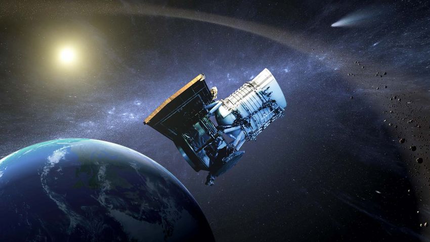
NEOWISE mission overview
• PI-led (PI: Amy Mainzer, U Arizona) under
 NASA PDCO Program (Lindley Johnson,
 Planetary Defense Officer)
• Utilizes WISE spacecraft brought out of
 hibernation in October 2013, following same
 survey pattern
• 3.4 and 4.6 µm bands (W1 and W2) at ~77K
• Terminator-following pole-to-pole orbit
• Surveys entire sky roughly every 6 months
• Mission goals:
 • Expand survey of NEOs at mid-infrared
 wavelengths using W1 and W2 channels
 • Obtain physical characterization (including
 diameters and albedos) of NEOs detected by
 NEOWISE
 • NEOWISE observations a key component to future
 mission planning (both human and robotic) as well
 as planetary defense preparation
 NASA JPL/Caltech
Sizes from Thermal Infrared
Seven years of NEOWISE survey

 Masiero et al. in prep

NEO size accuracy
 • Sizes from NEATM are
 spherical equivalent
 diameters

 • Using only 3.4 and 4.6
 microns, NEO diameter
 accuracy is ~30-40%

 • This is due to uncertainty
 in the beaming parameter
 for NEOs

 • When thermal peak is
 observed and beaming can
 be fit (e.g. cryogenic WISE
 mission) diameter
 accuracy improves to ~10-
 15%

 Masiero et al. in prep
Albedo Uncertainty
 • Albedos derived by combining thermal IR diameters with
 optical measurements

 • Uncertainties from both components drive final albedo
 uncertainty

 • For NEOs, observations made at high phases result in
 large H mag uncertainties unless G slope parameter is
 constrained

 • This drives the uncertainty on albedo

 • For the Main Belt, optical observations are at low phase
 angles, so uncertainty on H much smaller, and not
 comparable to NEOs

 • Caution needed when relating albedo to physical
 properties

 • See Masiero et al. 2021, PSJ, 2, 32 for discussion Masiero et al 2021

Observations of Exercise Object 2021 PDC

 • NEOWISE would not detect 2021 PDC in regular survey
 operations
 • However, a survey replan would allow NEOWISE to follow it for
 ~3 weeks in June 2021
 • This would allow for 300 exposures of 2021 PDC, which could be
 coadded to increase sensitivity
 • Trade off would be increased heat load on the telescope potentially
 reducing sensitivity by the end of the observing campaign
 • Data would be sufficient for a 3σ detection of a 100m size object

 INFORMATION ON THIS SLIDE REFERS ONLY TO A THEORETICAL PLANNING EXERCISE
Size constraints on 2021 PDC
 • Using an assumed 3σ detection, NEATM thermal model fit
 gives a diameter of 2021 PDC of 160 ± 80 m
 • Large uncertainty a result of unknown beaming parameter
 • Based on this, NEOWISE would be able to provide a 3σ upper
 limit of D < 240 m to mitigation planners by early July 2021
 • As data came in over June, upper limit could be calculated and
 would steadily decrease, with largest sizes being rejected in mid
 June

 INFORMATION ON THIS SLIDE REFERS ONLY TO A THEORETICAL PLANNING EXERCISE
Conclusions
 • NASA has requested that the NEOWISE team plan to continue
 survey through June 2023
 • Orbital evolution will be monitored as sun comes out of Solar
 minimum
 • NEOWISE continues to perform well
 • No significant degradation in sensitivity anticipated during this
 time, rate of NEO characterization expected to continue at
 current level
 • NEOWISE offers a unique capability to provide thermal IR
 observations of a large number of NEOs in support of hazard
 assessment and planetary defense
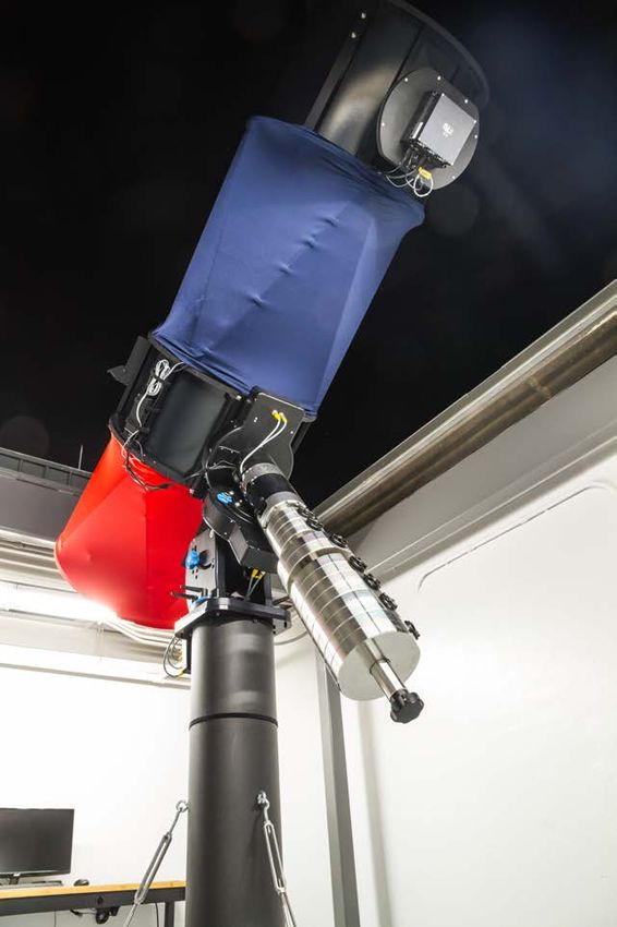
Polarimetry as a tool for physical
 characterization of potentially
 hazardous NEOs

 Maxime Devogèle1 & Nicholas Moskovitz2
1Arecibo Observatory/University of Central Florida
 2Lowell Observatory

 Planetary Defense Conference 2021
 April 27, 2021
 Image credit: Israel Cabrera Photography
What is polarimetry?

 Measure of the linear
polarization of the sun-
 light scattered by the
surface of an asteroid
What is polarimetry?

Polarimetry is mainly
 dependent on the
 phase angle
Why polarimetry is important?

 The phase-
polarization curve is
 dependent on the
 albedo
NEOs observations in polarimetry

 NEOs can be observed at
 higher phase angles

 NEOs

 MBA
Polarimetry-Albedo relation
 Bowell et al. 1973

 The Umov law is
 liking the albedo to
 Albedo

 the maximum of
 polarization

 Pmax
Polarimetry-Albedo relation

 50
 Polarization

 10

 1

 30 40 50 60 70 80 90 100
 Phase angle
Polarimetry-Albedo relation
 Ryugu
 50 Bennu
 1998 KU2
 Phaethon
 Polarization

 10
 Albedo ~ 0.02 - 0.1

 1

 30 40 50 60 70 80 90 100
 Phase angle
Polarimetry-Albedo relation

 50 Albedo < 0.02 - 0.1 2021 PDC: 150m
Polarimetry-Albedo relation

 50 Albedo < 0.02 - 0.1 1999 JD6
 Albedo ~ 0.14
 Polarization

 10

 1

 30 40 50 60 70 80 90 100
 Phase angle
Polarimetry-Albedo relation

 50 Albedo < 0.02 - 0.1
 Albedo ~ 0.1 - 0.15
 2021 PDC: 120m
Polarimetry-Albedo relation

 50 Albedo < 0.02 - 0.1 Mostly S-type
 Apophis
 0 . 15 Itokawa
 -
 Polarization

 10 0 .1 Eros
 o ~
 lb e d
 A Toro
 Ivar
 …
 1
 Albedo~
 0.15-0.35
 30 40 50 60 70 80 90 100
 Phase angle
Polarimetry-Albedo relation

 50 Albedo < 0.02 - 0.1

 0 . 15 Albedo ~ 0.15 - 0.4
 -
 Polarization

 10 ~ 0.1
 e d o
 A lb 2021 PDC: 80m
Polarimetry-Albedo relation

 50 Albedo < 0.02 - 0.1

 0 . 15
 -
 Polarization

 10 0 .1
 o ~ 0. 4
 lb e d
 15 -
 A 0 . 1999 WT24
 o ~
 lb e d 2004 VD17
 A
 …
 1
 Albedo~
 0.45-0.75
 30 40 50 60 70 80 90 100
 Phase angle
Polarimetry-Albedo relation

 50 Albedo < 0.02 - 0.1

 0 . 15
 -
 Polarization

 10 0 .1
 o ~ 0. 4
 lb e d
 15 -
 A 0 .
 o ~
 lb e d
 A 2021 PDC: 50m
Conclusions

 •Polarimetry is very effective to obtain albedo information
 •One measurement can reduce the size uncertainty by a factor
 of 2 to 10
 •We need new observations to better calibrate the polarimetry-
 albedo relation
 •We need more polarimeters on large aperture telescopes
Challenges in Differentiating NEOs and
 Rocket Bodies: 2020 SO Study

 Presented by Prof. Vishnu Reddy, University of Arizona
 Team: Adam Battle, Peter Birtwhistle, Tanner Campbell, Paul Chodas, Al Conrad, Dan Engelhart, James Frith,
Roberto Furfaro, Davide Farnocchia, Ryan Hoffmann, Olga Kuhn, David Monet, Neil Pearson, Jacqueline Reyes,
 Barry Rothberg, Benjamin Sharkey, Juan Sanchez, Christian Veillet, Richard Wainscoat
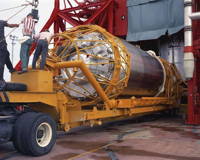
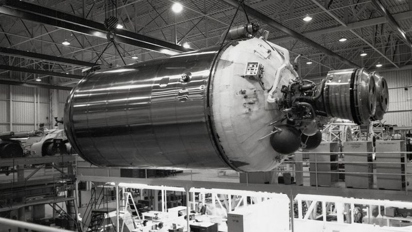
2020 SO: Background
• Discovered by PanSTARRS 1 telescope in
 Hawaii on September 17, 2020

• Temporarily captured on Nov. 8, 2020

Two close approaches:
• Inbound approach on December 1, 2020
 at a distance of 0.13 LD (50,414 km)

• Outbound approach on February 2, 2021
 at a distance of 0.58 LD (225,144 km) • Launched September 20, 1966 from
 KSC, Florida
• Low orbital velocity and Earth like orbit
 Paul Chodas suggested this could be • Centaur upper stage went into
 artificial object (Surveyor 2 Centaur heliocentric orbit similar to the Earth
 rocket booster)
 Atlas-Centaur Centaur D 2nd Stage Dimensions:
 Length: 9.6 meters
 Diameter: 3.05 meters
 Unfueled Mass: 2631 kgs
Goals and Challenges
Study Goals:
• Is 2020 SO an asteroid or rocket body?
• If it is a rocket body, is it a Centaur upper stage from Surveyor 2?
Challenges:
• Observability: 2020 SO was too faint for traditional near-IR characterization till mid-Nov.
 Late Sept. 2020 it was at V. Mag. 21.5, which limited us to broadband colors.
• Can you tell the difference between an asteroid and rocket body with colors?
• Spectral Interpretation: Do we have relevant spectral libraries of analog materials to verify
 if 2020 SO is a Centaur R/B? Especially something that had been in space for 54 years?
Observability Plot and Table

 Date (UTC) Target V. Mag. Phase Angle Range (km) Range (LD) Telescope Aperture Instrument Type of Observations Wavelength Range Spec. Res.
 28-Sep-20 2020 SO 21.5 20.5 3420234 8.898 LBT 8.2-m LBC Sloan griz colors 0.464-0.90 µm R=4
 10-Oct-20 NORAD ID: 3598 ~6-8 76.8 745 0.002 RAPTORS I 0.6-m FLI 4220 Visible spectroscopy 0.438-0.950 µm R~30
 22-Oct-20 NORAD ID: 6155 ~6-8 15.5 1300 0.003 RAPTORS I 0.6-m FLI 4220 Visible spectroscopy 0.438-0.950 µm R~30
 17-Nov-20 NORAD ID: 4882 ~6-8 80.6 4900 0.013 RAPTORS I 0.6-m FLI 4220 Visible spectroscopy 0.438-0.950 µm R~30
 17-Nov-20 2020 SO 19.3 21.9 1160736 3.020 NASA IRTF 3.0-m SpeX Near-IR spectroscopy 0.69-2.54 µm R~100
 29-Nov-20 2020 SO 15.7 5.4 300896 0.783 NASA IRTF 3.0-m SpeX Near-IR spectroscopy 0.69-2.54 µm R~100
 30-Nov-20 2020 SO 14.9 5.5 152894 0.398 NASA IRTF 3.0-m SpeX Near-IR spectroscopy 0.69-2.54 µm R~100
 30-Nov-20 NORAD ID: 4882 ~6-8 62.4 34000 0.088 NASA IRTF 3.0-m SpeX Near-IR spectroscopy 0.69-2.54 µm R~100
 2-Feb-21 2020 SO 15.8 23.8 221541 0.576 NASA IRTF 3.0-m SpeX Near-IR spectroscopy 0.69-2.54 µm R~100
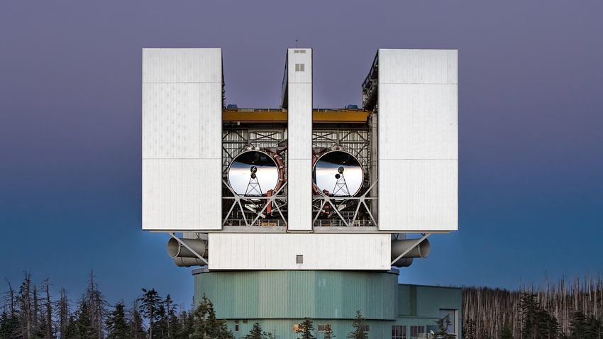
Color Observations Study Lead: Ben Sharkey (grad student)

• Large Binocular Telescope: Two
 8.2 meter optical/IR telescopes
• Instrument: Large Binocular
 Camera (red) and (blue) for color
 photometry (Sloan) and
 g’r’ i’z’
 astrometry
• Exposure times: 60 seconds
• Visual Magnitude: 21.5
• Images: 10 per filter
• Filters: Sloan g’r’I’z’
 Mt. Graham, AZ
• SNR: ~15 for g’r’i’; 10 for z’
Color Observations Study Lead: Ben Sharkey (grad student)

• Large Binocular Telescope: Two
 8.2 meter optical/IR telescopes Comparison with S-type and D-type asteroids

• Instrument: Large Binocular
 Camera (red) and (blue) for color
 photometry (Sloan) and
 astrometry
• Exposure times: 60 seconds
• Visual Magnitude: 21.5
• Images: 10 per filter
• Filters: Sloan g’r’I’z’
• SNR: ~15 for g’r’i’; 10 for z’
Visible Spectral Observations Study Lead: Adam Battle (grad student)

• Goal: Observe another Centaur in Earth orbit from the
 same period and compare with LBT color spectrum of
 2020 SO
• RAPTORS: Robotic Automated Pointing Telescope for
 Optical Reflectance Spectroscopy
• Telescope: 0.6-meter F/4.6 Newtonian optical/NIR
 telescopes (RAPTORS I and II)
• Instrument: FLI4210 CCD and Richardson Grating 30L
 transmission grating giving a spectral resolution R~30
• Exposure times: 0.01-1.0 seconds (Object kept in the
 center to make sure there are no shutter effects)

 Tucson, AZ
Comparison with Centaur R/Bs
Here are the visible wavelength spectra of the three Centaur bodies NORAD
ID 3598, 4882 and 6155. 3598 was launched in 1968, 4882 in 1971 and 6155
in 1972. All Centaur spectra are consistent with each other. Differences at
the shortest and longest wavelengths could be due to phase angle.
Near-IR Observations Mauna Kea, HI

• NASA IRTF: 3-meter IR telescope
• Instrument: SpeX spectrometer
• Exposure times: 200 seconds
• Visual Magnitude: 19.3, 15.7,
 14.9 and 15.8
Near-IR Observations Study Lead: Juan Sanchez (post doc)

• First spectrum of 2020 SO (V. Mag.
 19.3) obtained at the limit of
 IRTF’s capabilities (V. Mag. 19.5)
• Steep red slope till 1.5 µm
• No major absorption features
 detected, possible weak ones
• Diagnostic absorption bands key
 to constraining composition
• Compared LBT 2020 SO data and
 RAPTORS spectra of Centaur R/Bs
• Consistent with NASA IRTF data
Near-IR Observations
• Next two spectra of 2020 SO were
 obtained days before close
 approach (Dec. 1, 2020)
• Spectral slope consistent with
 Nov. 17 data
 2.29 µm
• Major absorption bands are seen 1.72 µm
 1.42 µm
 in spectra from Nov. 29, 30.
• Diagnostic absorption bands key
 to constraining composition
• Bands are located at 1.42±0.02,
 1.72±0.01 and 2.29±0.01 µm
• But we did not have good lab
 spectral of analog materials
Near-IR Observations
• Spectrum of Centaur R/B (4882)
 consistent with 2020 SO
• Red spectral slope with
 absorption bands
• Absorption features at 1.42±0.02, 2.29 µm
 1.72±0.01 are weaker in the 1.72 µm
 PA 62.4° 1.42 µm
 Centaur than 2020 SO.
• Spectral slope and absorption
 band depth difference could be
 due to phase angle differences or
 PA 5.4°
 space ageing
• What materials on 2020 SO is
 causing these absorption bands?
Study Lead: Neil Pearson (UA)
Interpretation 301 Stainless Steel
Spectrally-significant components

 301 Stainless Steel

 White polyvinyl fluoride

 Aluminized Mylar
Interpretation Object/
 Material
 Band I Center
 (µm)
 Band II Center
 (µm)
 Band III Center
 (µm)
 PVF (Lab) 1.432±0.001 1.716±0.001 2.307±0.001

 2020 SO 1.430±0.02 1.720±0.01 2.290±0.01

 Mylar loses the 0.8 µm
 absorption with age
 Dan Engelhart and creates red slope
 in the visible

 1.72 µm 2.29 µm
 1.42 µm

 Stainless Steel also has red spectral
 slope similar to aged Mylar
Summary
• We have demonstrated the power of spectroscopy in differentiating natural vs. artificial
 objects in near-Earth space.

• Fast turn around (2 weeks) for 2020 SO characterization (Asteroid Yes/No) after discovery
 (LBT color observations).

• Space ageing/weathering remains a major challenge in our ability to interpret 2020 SO
 spectra.

• We will attempt spectral mixing models once we have better end member lab spectra.

 Acknowledgment: This work was funded by NASA Near-Earth Object Observations Grant NNX17AJ19G (PI: Reddy).
Backup Slides
Lightcurve Observations

 No clear evidence for a rotational period
 Maybe a fast rotator or tumbling?
Lightcurve Observations

 Great Shefford Obs.
 RAPTORS II

 Close Approach 1, Range 94,000 km Close Approach 2, Range 360,000 km
Color Observations
• Is the Centaur D Stage really painted white?
Color Observations
 • If it is not white paint what is
 it?
 • Phillip Anz-Meador (Jacobs,
 at NASA JSC)
 • “Centaur D (operational)
 models jettisoned the foam
 insulation panels revealing
 the SS underneath”
 • 2020 SO should be made of
 Stainless Steel 301.
Visible Spectral Observations
Centaur D History: 24 Centaur D upper stages were launched between Aug. 1965 and
Aug. 1972. Eight of which remain in Earth orbit. The three we picked were based on
their visibility from Tucson. Two in LEO orbits were extremely challenging for
spectroscopy, third was in GTO and easier to track at apogee.
 Apogee Perigee
 Inclination
Launch Vehicle Seq. Name Launch Date Primary Payload NORAD ID Period (Min) Altitude Altitude
 (Deg)
 (km) (km)
 Atlas-LV3C AC-11 14 JUL 1967 Surveyor 4 2883 113.38 64.66 2499 265
 Atlas-SLV3C AC-16 07 DEC 1968 OAO 2 3598 99.00 34.99 746 676
 Atlas-SLV3C AC-18 12 AUG 1969 ATS 5 4069 703.13 17.88 37299 2331
 Atlas-SLV3C AC-25 26 JAN 1971 Intelsat-4 2 4882 652.52 27.33 36499 585
 Atlas-SLV3C AC-26 20 DEC 1971 Intelsat-4 3 6779 655.72 28.31 36599 648
 Atlas-SLV3C AC-28 23 JAN 1972 Intelsat-4 4 5816 651.92 27.78 36449 605
 Atlas-SLV3C AC-29 13 JUN 1972 Intelsat-4 5 6058 647.68 26.27 36294 543
 Atlas-SLV3C AC-22 21 AUG 1972 OAO 3 6155 97.85 35.01 682 630

Date (UTC) Target V. Mag. Phase Angle Range (km) Range (LD) Telescope Aperture Instrument Type of Observations Wavelength Range Spec. Res.
28-Sep-20 2020 SO 21.5 20.5 3420234 8.898 LBT 8.2-m LBC Sloan griz colors 0.464-0.90 µm R=4
10-Oct-20 NORAD ID: 3598 ~6-8 76.8 745 0.002 RAPTORS I 0.6-m FLI 4220 Visible spectroscopy 0.438-0.950 µm R~30
22-Oct-20 NORAD ID: 6155 ~6-8 15.5 1300 0.003 RAPTORS I 0.6-m FLI 4220 Visible spectroscopy 0.438-0.950 µm R~30
17-Nov-20 NORAD ID: 4882 ~6-8 80.6 4900 0.013 RAPTORS I 0.6-m FLI 4220 Visible spectroscopy 0.438-0.950 µm R~30
17-Nov-20 2020 SO 19.3 21.9 1160736 3.020 NASA IRTF 3.0-m SpeX Near-IR spectroscopy 0.69-2.54 µm R~100
29-Nov-20 2020 SO 15.7 5.4 300896 0.783 NASA IRTF 3.0-m SpeX Near-IR spectroscopy 0.69-2.54 µm R~100
30-Nov-20 2020 SO 14.9 5.5 152894 0.398 NASA IRTF 3.0-m SpeX Near-IR spectroscopy 0.69-2.54 µm R~100
30-Nov-20 NORAD ID: 4882 ~6-8 62.4 34000 0.088 NASA IRTF 3.0-m SpeX Near-IR spectroscopy 0.69-2.54 µm R~100
 2-Feb-21 2020 SO 15.8 23.8 221541 0.576 NASA IRTF 3.0-m SpeX Near-IR spectroscopy 0.69-2.54 µm R~100
Color Observations
 • Spectra of SS 301 obtained
 from AFRL (Dan Engelhart)
 • These spectra were not aged
 under the assumption that
 Stainless Steel won’t oxidize
 like Aluminum would.
 • Plot on the right compares
 2020 SO griz colors with
 Stainless Steel Tube.
 • Both have red spectral slopes,
 but 2020 SO is redder than lab
 spectrum of Stainless Steel.
Chasing Centaur Challenges
• Identifying specific materials TLE for 4882 was 2.5 days old
 requires extensive lab spectroscopy
 if we can get the material samples IRFT FOV
 Centaur position off by 8.15’ (8X
 IRTF FOV)
• How do spectra of materials change
 with space ageing? We tried to observe 4882 from
 my backyard a few hours before
• Logical solution was to observe IRTF observations but was too
 another Centaur with the IRTF, IRTF Tracking Limit: 40”/sec low in the sky.
 preferably one of three we observed Centaur Rates: RA Rate: 13 "/sec
 with RAPTORS I (visible spectra)
 Apogee Perigee
 Inclination
 Launch Vehicle Seq. Name Launch Date Primary Payload NORAD ID Period (Min) Altitude Altitude
 (Deg)
 (km) (km)
 Atlas-LV3C AC-11 14 JUL 1967 Surveyor 4 2883 113.38 64.66 2499 265
 Atlas-SLV3C AC-16 07 DEC 1968 OAO 2 3598 99.00 34.99 746 676
 Atlas-SLV3C AC-18 12 AUG 1969 ATS 5 4069 703.13 17.88 37299 2331
 Atlas-SLV3C AC-25 26 JAN 1971 Intelsat-4 2 4882 652.52 27.33 36499 585
 Atlas-SLV3C AC-26 20 DEC 1971 Intelsat-4 3 6779 655.72 28.31 36599 648
 Atlas-SLV3C AC-28 23 JAN 1972 Intelsat-4 4 5816 651.92 27.78 36449 605
 Atlas-SLV3C AC-29 13 JUN 1972 Intelsat-4 5 6058 647.68 26.27 36294 543
 Atlas-SLV3C AC-22 21 AUG 1972 OAO 3 6155 97.85 35.01 682 630 Tucson, AZ
ACCURATE NEO ORBITS FROM
 OCCULTATION OBSERVATIONS
 Paper IAA-PDC-21-6-09 (Session 6b, #4)

 7th Planetary Defense Conference – PDC 2021
 26-30 April 2021, Vienna, Austria and via Webex
 David W. Dunham1&2, J. B. Dunham1, M. Buie3, S. Preston1, D. Herald1,4, D. Farnocchia5, J.
 Giorgini5, T. Arai6, I. Sato6, R. Nolthenius1,7, J. Irwin1, S. Degenhardt1, S. Marshall8, J. Moore1, S.
 Whitehurst1, R. Venable1, M. Skrutskie9, F. Marchis10, Q. Ye11, P. Tanga12, J. Ferreira12, D.
 Vernet12, J.P. Rivet12, E. Bondoux12, J. Desmars13, D. Baba Aissa14, Z. Grigahcene14,
 and H. Watanabe15
 1International Occultation Timing Assoc. (IOTA, P. O. Box 423, Greenbelt, MD 20768, USA,

iotatreas@yahoo.com), 2KinetX Aerospace (david.dunham@kinetx.com), 3Southwest Research
 Inst., Boulder, CO, 4Trans Tasman Occultation Alliance, 5Jet Propulsion Lab., 6Planetary
 Exploration Res. Ctr. (PERC), Chiba Inst. of Tech., Japan, 7Cabrillo College, Santa Cruz, CA,
8Arecibo Obs., 9Univ. of Virginia, 10SETI Inst. and Unistellar, 11Univ. of Maryland,12Obs. de la Côte

 d'Azur, 13Paris Obs., 14Algiers Obs. – CRAAG, 15Japanese Occultation Information Network

 Version of 2021 April 26, 7pm EDT
Outline • IOTA & Asteroidal Occultations Introduction & History • The 1975 Jan. 24 Occ’n of Gem by Eros • The 2019 July Occ’n by Phaethon, 1st small NEO occ’n • Other Phaethon occultations, 2019 Sep. to 2020 Oct. • Improvement of Phaethon’s orbit – A2 acceleration • More Opportunities in 2021 & 2022 • First Observed Occultation by Apophis, 2021 Mar. 7 • Almost lost it – 2nd Positive Occ’n, 2021 Mar. 22 • 2021 April Occultations – Apophis Orbit Nailed • Conclusions • Additional Resources
IOTA and Asteroidal Occultations Introduction
• The observer network that became IOTA formed in 1960’s
• to observe lunar grazing occultations with mobile efforts
• The mobile techniques to observe lunar grazes, were used effectively to
 observe asteroidal occultations in the late 1970’s
• Starting in the 1980’s, IOTA began recording occultations with video
 equipment, improving the observations
• Using stars and the Earth’s rotation to pre-point stationary telescopes at
 multiple locations
• Working with the NASA PDS Small Bodies Node and the Minor Planet
 Center, IOTA archives all asteroidal occultation observations
• ESA’s Hipparcos and Gaia missions have greatly improved prediction
 accuracy, resulting in a large increase in observed occultations
• The sizes, shapes, and accurate positions of hundreds of asteroids have
 been determined
• Dozens of close double stars have been discovered, the diameters of
 several stars have been measured, and some asteroidal satellites have
 been discovered, and several characterized.
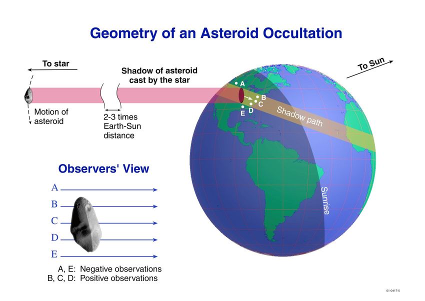
Lunar Occultation Geometry
 IOTA started in the early 1960’s by observing lunar
 occultations, especially grazing ones

 B – Has no occultation (a miss)
 C – Tangent path, a Grazing Occultation
 A – Total Occultation
Lunar Profile from Graze of delta Cancri – 1981 May 9-10 Alan Fiala, USNO, obtained the first video recording of multiple events during this graze, with 7 D’s and 7 R’s During the 4 min., the Moon moved 250 km so the vertical Expeditions like this inspired a generation of young scale is about amateur astronomers before & after the Apollo missions 40 times the horizonal scale A good example of a graze is shown by a composite video of the 2017 Mar. 5th Aldebaran graze at https://vimeo.com/209854850 Circled dots are Watts’ predicted limb corrections
Starting in 1965, cable systems were developed for
 observing grazing occultations, first at USNO, then by 3
 clubs in California (Riverside, Santa Barbara, and Mount
 Diablo Astronomical Society), and Milwaukee, Wisconsin

This is a Riverside A.S. expedition near Adelanto in 1966. Mobile observation
was needed since graze paths were narrow. The observations were visual,
with audio tones recorded at the central station for this cable system.
IOTA began observing asteroidal occultations in the late 1970’s

 The more stations that can be
 deployed, the better the resolution
 of the asteroid’s shape
Many Occultations of Interesting Main Belt Objects
2011 July 19 occ’n of LQ Aquarii by Technology now allows observers to record
 transient astronomical phenomena more
 the Binary Asteroid (90) Antiope precisely and to fainter magnitudes than ever
 before. A small, inexpensive, yet very sensitive
 camera (RunCam Night Eagle Astro) will allow
 you to participate in IOTA’s programs to
 accurately record occultations and eclipses, to
 measure the sizes and shapes of hundreds of
 asteroids, discover duplicity of both close
 double stars and asteroids with satellites, and
 measure the angular diameters of many stars.
 Occultations provide excuses for travel, or you
 can just observe them from home, to further
 astronomical knowledge. Some use specially-
 made easily-transported telescopes; there is
 room for innovative design & construction of
 equipment & software to record asteroidal
 occultations.
 Near left: 10-in
 suitcase tele-
 scope deployed
 for an asteroidal
 occultation in
 the Australian
 8
 Outback.
Remote Stations for Asteroidal Occultations • Separation should be many km, much larger than for grazes, so tracking times & errors are too large • Unguided is possible since the prediction times are accurate enough, to less that 1 min. = ¼ (now the prediction time errors are only a few seconds) • Point telescope beforehand to same altitude and azimuth that the target star will have at event time and keep it fixed in that direction • Plot line of target star’s declination on a detailed star atlas; Guide 8 or 9, or C2A can be used to produce the charts • From the RA difference and event time for the area of observation, calculate times along the declination line • Adjust the above for sidereal rate that is faster than solar rate, add 10 seconds for each hour before the event; done automatically by Guide & C2A • Can usually find “guide stars” that are easier to find than the target • Find a safe but accessible place for both the attended & remote scopes • Separation distance limited by travel, set-up, & pre-pointing time, but we have had success with software to control small Win10 computer recordings; then the main limit is battery life, which can be several hours • Sometimes it is better to have remote sites attended for starting equipment later (allows larger separations) and security, if enough people can help
First observed occultation by a NEO, 1975 Jan. 24, Gem occulted by Eros from O’Leary et al., Icarus, Vol. 28, pp. 133-146 (1976) Left, map of observers & sky plane plot from the 1976 Icarus paper. Right, modern sky plane plot of the chords fitted to Eros’ shape model derived from NEAR- Shoemaker data. This was the first occultation by ANY asteroid that was observed from multiple stations. Especially, the stations deployed by the Pioneer Valley Colleges led by Brian O’Leary was the first successful coordinated effort to observe such an event by mobile observers. A crucial observation, now known to be a false negative, resulted in the wrong squashed shape shown by O’Leary et al. It would be 44 years before an occultation by another NEO would be observed.
(3200) Phaethon
• (3200) Phaethon was the first asteroid to be discovered by a spacecraft (IRAS).
• Phaethon is the parent body of the Geminids meteor stream that puts on one of
 the largest annual meteor displays
• This mysterious object may be a (nearly) dead comet nucleus, or a very active
 asteroid, throwing off boulders like has been observed on Bennu by OSIRIS-REx
• Phaethon is an Apollo asteroid with a perihelion of only 0.14 AU,
THE 2019 JULY 29 OCC’N OF 7.3-MAG. SAO 40261 BY PHAETHON • This event was first identified by Isao Sato in Japan. In January 2019, he alerted US observers via a message that he sent to the IOTAoccultations list server. • To obtain an accurate astrometric point for orbit improvement, and to resolve the diameter discrepancy, Tomoko Arai, PI of DESTINY+, requested that NASA & IOTA try to observe this rare bright occultation by the small NEO in the sw USA. • This was by far the smallest object that IOTA had tried to predict and observe; we needed help. • Those who predicted this occultation, and analyzed the observations of it, all had to modify their software, to take into account previously-neglected effects that weren’t significant for occultations by all of the larger objects studied in the past. Even the difference in the gravitational bending of light by the Sun, for the star and Phaethon, was noticeable. • Jon Giorgini computed JPL solution 684 after including radar measurements made in 2017. Then Davide Farnocchia computed JPL 685, manually adding Gaia astrometry; this was key. • Adding new astrometric observations just confirmed JPL 685, so it was used for the final prediction. 3- error ellipses for JPL sol’ns in July 29 Prediction by sky plane S. Preston, IOTA [Daylight] Phaethon’s motion was from lower left to upper right, → so the 3 limits (JPL 685) were 8 km + Phaethon’s radius from center; the ground projection was a little larger. D. Farnocchia
2019 July 29 Phaethon occ’n, all successful chords
2019 July 29 Phaethon occultation, positive chords
 fitted to a shape model determined from 2017 December Arecibo radar observations

 by
 Dave Herald and
 Sean Marshall

The event provided accurate information about Phaethon’s size (verifying the radar
value), shape, and orbit that will be valuable for DESTINY+’s planning, and will help
obtain more data from future occultations that can be better predicted.
To ensure success, the first event needed a deployment across 4 States by scores of
professional and amateur observers, forming a network of stations with an unprecedentedly
small spacing between them. After the 2019 July 29th success, it was possible to predict the Sept.
29th event, and then each of the others, with better improvement each time as more observations
were added to the orbit solutions.
“Star mag.” measures the star’s magnitude, with lower numbers for brighter stars, like rankings. The first
event was visible with binoculars; all the others needed telescopes.
Positive chords recorded the occultation, while all includes negative observations; SCT= Scmidt-
Cassegrain Telescope.
More about these observations is in the longer presentation I gave at the 2020 meeting
of the International Occultation Timing Association. It is the 4th from the bottom, on the 2020 IOTA 7
presentations page at:
http://occultations.org/community/meetingsconferences/na/2020-iota-annual-
meeting/presentations-at-the-2020-annual-meeting/ .
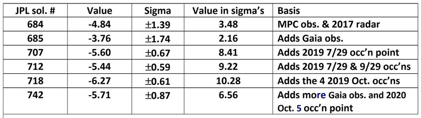
Phaethon Orbit A2 Determinations
 (units au/d^2 x10-15)

The A2 term for most NEO’s is caused by the Yarkovsky effect,
but for Phaethon, mass loss due to strong thermal heating near
perihelion is likely the main driver, as evidenced by the Geminids
& the Phaethon dust trail imaged by the Parker Solar Probe.
Future Phaethon Occultations

Predictions for 10 more Phaethon occultations in late 2021 are at
http://iota.jhuapl.edu/2020-2022Phaethon.htm, including the one above.
Occultations by (99942) Apophis
• Discovered in 2004; very close approach in 2029 identified
• Elongated object, about 350m x 170m, from 2011 radar obs.
• 2029 flyby near ring of geosats; no threat, but great sci. opp.
• But could pass through “keyhole” into a resonant orbit
• With the best orbit before 2021, small chance of 2068 impact
• If impact, total destruction to 25km; severe damage to 300 km
 Paris Obs.’s Lucky Star Project found a
 7th-mag. occ’n across N. America on 2021
 Feb. 22, but without radar, it could not be
 predicted well. They found another event,
 star mag.8.4, with map at
 left, and radar data were
 expected a few days before.
 The shape model with new
 spin state, aspect for the
 event from Marina Borzovic,
 is at right.
 Much information about past observed Apophis occultations, and predictions for
 future ones, are at http://iota.jhuapl.edu/Apophis2021.htm.
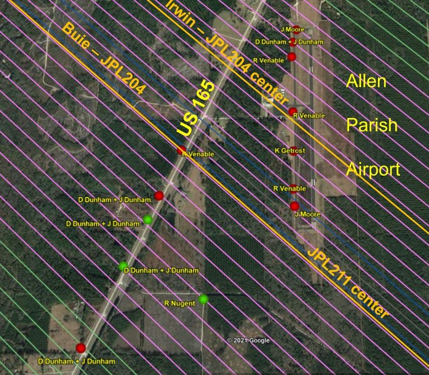
2021 March 7 Stations near Oakdale, Louisiana
 6 IOTA observers deployed telescopes
 at a small airport and along US 165
 south of Oakdale, Louisiana. Red dots
 mark stations that had a miss, while 3
 green dots mark 3 that recorded the
 occultation. The station locations were
 selected to be close to the diagonal
 tracks shown on the map, 107 meters
 apart as projected on the ground. They
 were 80 meters apart on the plane of
 the sky. J. Moore pre-pointed 2 systems
 that recorded the star, R. Venable 4,
 and D & J Dunham, 5, 2 of which
 (green dots) recorded the occulta-
 tion, as did R. Nugent between
 them. K. Getrost recorded a miss.
Orange lines show 3 predictions, two based on JPL orbit 204 computed on March 5
refined with the radar obs. made the previous 3 nights. JPL orbit 211 shows a later
prediction that should be close to where the path would have been, if the Gaia
position for NY Hydrae had been correct, as noted below. Some of the lines were
covered by observers in Oklahoma, Colorado, and British Columbia; their
observations were all negative.
Dunham “Mighty Midi” Systems at A30 & A28 A30 A28 PC164C-EX2 Camera batteries IOTA VTI Runcam iView David and Joan Dunham’s equipment used on line A30 (northern, left) and line A28 (southern, right). Both stations used 80mm f/5 refractors with f/0.5 focal reducers, small video cameras, an IOTA video time inserter (VTI) for accurate time- stamping of the videos with GPS 1PPS (the VTI is under the towel at A28), and iView “stick” Win10 computers to record the video. Except for the cameras, the equipment was the same at the two stations. These pictures were taken during a practice run at their home 3 nights before the occultation.
Venable’s 2021 Mar. 22 stations, Yeehaw Jct., Florida

The March 7th observations were quickly analyzed to update the orbit, as 4 nights later,
there was an Apophis occultation in Europe. Two observers from Thessaloniki, Greece
traveled to the path predicted by the new orbit JPL207, but both had a miss. On March
22nd, an occultation of a 10.0-mag. star was predicted for the eastern USA. Some tried
the event in n.e. Alabama and Illinois, where they had a miss. R. Venable deployed 5
telescopes near Yeehaw Junction, Florida, as shown above. Only his easternmost
telescope recorded the occultation. The path between the blue lines was computed
from JPL orbit 207 (updated using the March 7th observations) and used for planning.
The better path between the yellow lines was computed later from JPL orbit 214a that
used later occultation observations. By spreading his scopes out enough, Venable
saved Apophis’ accurate orbit; the JPL 207 error apparently was due to error in Gaia’s
position of NY Hya caused by its duplicity (eclipsing binary) that was occulted on Mar. 7.
2021 April 11 Apophis occultation in New Mexico

With Apophis’ orbit nailed by the April 4th observations, we were able to
accurately locate the three observers, each with one telescope, for the
April 11th occultation of a 10.1-mag. star, so that each had occultations.
Above is Kai Getrost’s light curve of the occultation that was recorded
with 100 frames per second from Farmington, New Mexico with a QHY
174M GPS camera attached to a 20-inch Dobsonian telescope. Effects
of Fresnel diffraction are evident.
Summary of all observed positive Apophis occultations
 with O-C’s from JPL 214a

We believe HY Hydrae’s duplicity, more than the RUWE value, is the main explanation of the large
residuals on Mar. 7. Slide 17 shows the path (JPL 211, which was almost the Same as JPL 214a)
that would have occurred on March 7th, if the Gaia position of NY Hydrae had NOT been in error.
That threw us off after that event, causing the observers in Greece for the Mar. 11 occultation, to be
in the wrong place and have a miss. Fortunately, Venable was able to spread his stations out far
enough on Mar. 22 to catch that occultation (slide 19). The table shows that the residuals for March
7th stick out like a sore thumb, demonstrating the astrometric power of observations of occultations
by small NEOs.
Occultations helped retire the risk of Apophis
 Gaia Image of the week,
 2021 Mar. 29. “Apophis’
 Yarkovsky acceleration
 improved through stellar
 occultation”
 Also, please see Tanga et
 al’s poster, “Stellar
 occultations by NEAs,
 challenges and
 opportunities” that notes,
 DART/Hera target Didymos
 should be next for occ’ns
Evolution in time of our knowledge of the average Yarkovsky acceleration for 99942
Apophis. The light blue data represent the early theoretical estimates from approximate
models of the physical properties of Apophis1. The other data are measurements
enabled by the collection of more optical and radar astrometry. On the horizontal axis,
close encounters with the Earth (enabling collection of accurate astrometry) are marked.
The inset shows the last estimates compared to our value, in red, obtained from all the
observations available on March 15, including the occultation observed on March 7, 2021.
For more, see https://www.cosmos.esa.int/web/gaia/iow_20210329.
Predictions of future Apophis occultations

During June, July, and August, Apophis is too close to the Sun so no observable
occultations occur then. In September, the event durations become much shorter
so only brighter stars have a reasonable chance to be observed with video.
Maps and path details are on the IOTA Apophis page at
http://iota.jhuapl.edu/Apophis2021.htm
•
 Conclusions
 The rare bright 2019 July 29 occultation was the first successful campaign for a small
 th

 NEO; it’s the smallest asteroid with multiple timed chords during an occultation. One of
 the largest collaborations of amateur and professional astronomers for an occultation
 enabled this success.
• The radar size and shape were verified, and the improved orbit allowed a good
 prediction for the Sept. 29th occultation, then subsequent events, and an improvement
 of Phaethon’s A2 non-gravitational parameter by a factor of 3.
• Recently, the occultation technique was successfully applied to Apophis, which is
 more than 10 times smaller than Phaethon, further demonstrating the astrometric
 power of observations of NEO occultations for planetary defense.
• Information about the sizes, shapes, rings, satellites, and even atmospheres of Kuiper
 Belt objects, Centaurs, Trojans, and other asteroids is proportional to the number of
 stations that can be deployed for occultations by them
• So we encourage as many others as possible to time occultations by TNO’s and by
 other asteroids from their observatories
• We want students to learn to make the necessary mobile observations, including the
 multi-station techniques pioneered by IOTA, to observe NEO occultations; someday,
 one or more of them might observe an occultation that will save the world, or part of it.
• We hope that the pursuit of NEO occultations will inspire a new generation of
 astronomers to learn, apply, & improve the techniques for mobile occultation
 observation, like lunar grazing occultations did for us in the 1960’s and 1970’s.
• A longer more detailed version of this presentation (Power Point) is at
 http://iota.jhuapl.edu/PDC2021NEOoccultationsDunhamPresentationLong.pdf
•
 Additional Resources
 A longer and more detailed version of the Phaethon presentation is available, 4th from
 the bottom, on the presentations page of the 2020 IOTA meeting at:
 http://occultations.org/community/meetingsconferences/na/2020-iota-annual-
 meeting/presentations-at-the-2020-annual-meeting/ Another interesting talk there
 describes a fully automatic portable system, by A. Knox, the 4th from the top.
• IOTA Apophis occultations Web page: http://iota.jhuapl.edu/Apophis2021.htm
• MNRAS paper about IOTA’s/NASA’s asteroidal occultation archive and results:
 https://arxiv.org/abs/2010.06086
• IOTA main Web site, especially the observing pages: http://occultations.org/
• Occult Watcher for finding asteroidal occultations for your observatory and area, and
 for coordinating observations: http://www.occultwatcher.net/
• Link to George Viscome’s occultation primer:
 http://occultations.org/documents/OccultationObservingPrimer.pdf
• IOTA YouTube videos (Tutorials and notable occultations):
 http://www.asteroidoccultation.com/observations/YouTubeVideos.htm
• SwRI Lucy Mission Trojan occultations Web site (SwRI expeditions planned for many
 of them): http://lucy.swri.edu/occultations.html
• RECON TNO/Centaur occultations Web site (Mainly, w. USA events):
 https://www.boulder.swri.edu/~buie/recon/reconlist.html
• Lucky Star TNO/Centaur/Trojan occultations Web site: https://lesia.obspm.fr/lucky-
 star/predictions.php

 Updated 2021 April 26, 7pm EDT
A New Method for Asteroid Impact Monitoring
 and Hazard Assessment

 Javier Roa Vicens, Davide Farnocchia, and Steven R. Chesley
 j a v i e r. r o a @ j p l . n a s a . g o v
 7th IAA Planetary Defense Conference
 (Virtual) April 26-30, 2021
Introduction
Motivation for a new impact monitoring algorithm

 Goal of Impact Monitoring Challenges
 Identify and characterize all virtual 1. Many VIs that must be separated.
 impactors (VIs) compatible with the 2. Impact probabilities (IP) are usually
 orbital uncertainty distribution. small (~10–7).
 3. Nongravitational parameters must
 VI: region in parameter space leading to be handled automatically.
 impacts along the same dynamical path.* 4. Pathological cases (Earth-like
 orbits, nonlinearities).
 Uncertainty
 Projection in parameter space

 region
 Virtual
 impactors • Monte Carlo:
 1. 2. 3. 4.
 • Line of Variations (LOV):*
 1. 2. 3. 4.
 Nominal
 asteroid orbit
 Increased rate of NEA discoveries calls
 for a more robust method
 *Milani, A. et al. (2005): “Nonlinear impact monitoring: line of variation searches for impactors,” Icarus, 173, 362-384

 04/27/2021 © 2021 California Institute of Technology. Government sponsorship acknowledged. 2 jpl.nasa.gov
Impact Pseudo-Observation I
Finding VIs using an orbit-determination program

 Add Impact pseudo- Impact pseudo-observation
 Observations
 observation
 Add the impact condition as an
 observation:
 Orbit Orbit • The residuals are the B-plane
 determination determination
 coordinates at the time of close
 approach.
 Nominal orbit Impacting orbit • The uncertainty is a fraction of
 + covariance + covariance the Earth radius.

 • No simplifying assumptions about the dynamics or the uncertainty distribution in
 parameter space.
 • The covariance of the fit approximately models the VI in parameter space.
 • Use the same operational OD program used to produce the nominal orbit.

 04/27/2021 © 2021 California Institute of Technology. Government sponsorship acknowledged. 3 jpl.nasa.gov
Impact Pseudo-Observation II
Finding VIs using an orbit-determination program

 1- covariance
 Constrained of the impacting
 by data solution

 Impact
 obs.

 Earth
 cross-section

 04/27/2021 © 2021 California Institute of Technology. Government sponsorship acknowledged. 4 jpl.nasa.gov
Sentinel
A new automatic impact-monitoring system at JPL

 Operation of Sentinel

 1. Initial MC exploration: detect close approaches for further investigation.
 2. Find VIs: run OD filter extended with the impact pseudo-observation.
 3. Characterize the VIs: use importance sampling to estimate the IP.

 Features and Comparison with Sentry (LOV based)
 • Sentinel has been running and mirroring Sentry for a few months.
 • Sentinel handles nongravitational parameters systematically.
 • More robust in pathological cases.
 • Median runtimes for 100-year exploration and IP down to 10–7:
 o Monte Carlo: 14 days (20,000 min)
 o Sentry: 20 min
 o Sentinel: 40 min
 • Sentinel provides the nominal orbit and the uncertainty of each VI
 ⟹ useful for negative observation campaigns.

 04/27/2021 © 2021 California Institute of Technology. Government sponsorship acknowledged. 5 jpl.nasa.gov
j a v i e r. r o a @ j p l . n a s a . g o v
Q&A
Session 6b: NEO Characterization
End of Day 2
 Thank you
You can also read