Spatially Resolved Star Formation and Inside-out Quenching in the TNG50 Simulation and 3D-HST Observations

MNRAS 000, 1–15 (2021) Preprint 1 February 2021 Compiled using MNRAS LATEX style file v3.0

 Spatially Resolved Star Formation and Inside-out Quenching in the
 TNG50 Simulation and 3D-HST Observations
 Erica J. Nelson,1,2★ Sandro Tacchella,2 Benedikt Diemer,3 Joel Leja,4,5,6 Lars Hernquist,2
 Katherine E. Whitaker,7,8 Rainer Weinberger,2 Annalisa Pillepich,9 Dylan Nelson,10
 Bryan A. Terrazas,2 Rebecca Nevin,2 Gabriel B. Brammer,8,11 Blakesley Burkhart,12,13
 Rachel K. Cochrane,2 Pieter van Dokkum,14 Benjamin D. Johnson,2 Federico Marinacci,15
arXiv:2101.12212v1 [astro-ph.GA] 28 Jan 2021

 Lamiya Mowla,16 Rüdiger Pakmor,19 Rosalind E. Skelton,18 Joshua Speagle,16,18 Volker Springel,19
 Paul Torrey,20 Mark Vogelsberger,21 Stijn Wuyts22
 1 Department for Astrophysical and Planetary Science, University of Colorado, Boulder, CO 80309, USA
 2 Center for Astrophysics | Harvard-Smithsonian, Cambridge, MA 02138, USA
 3 Department of Astronomy, University of Maryland, College Park, MD 20742, USA
 4 Department of Astronomy & Astrophysics, The Pennsylvania State University, University Park, PA 16802, USA
 5 Institute for Computational & Data Sciences, The Pennsylvania State University, University Park, PA, USA
 6 Institute for Gravitation and the Cosmos, The Pennsylvania State University, University Park, PA 16802, USA
 7 Department of Astronomy, University of Massachusetts, Amherst, MA 01003, USA
 8 Cosmic Dawn Center (DAWN), Copenhagen, Denmark
 9 Max-Planck-Institut für Astronomie, Königstuhl 17, 69117 Heidelberg, Germany
 10 Universität Heidelberg, Zentrum für Astronomie, Institut für theoretische Astrophysik, Albert-Ueberle-Str. 2, 69120 Heidelberg, Germany
 11 Niels Bohr Institute, University of Copenhagen, Jagtvej 128, København N, DK-2200, Denmark
 12 Department of Physics and Astronomy, Rutgers University, 136 Frelinghuysen Rd., Piscataway, NJ 08854, USA
 13 Center for Computational Astrophysics, Flatiron Institute, 162 5th Ave., New York, NY 10010, USA
 14 Astronomy Department, Yale University, New Haven, CT 06511, USA
 15 Department of Physics and Astronomy “Augusto Righi", University of Bologna, via Gobetti 93/2, 40129 Bologna, Italy
 16 Dunlap Institute for Astronomy & Astrophysics, University of Toronto, Toronto, ON M5S 3H4, Canada
 17 South African Astronomical Observatory, Cape Town 7935, South Africa
 18 Department of Statistical Sciences, University of Toronto, Toronto, ON M5S 3G3, Canada
 19 Max-Planck-Institut für Astrophysik, 85740 Garching bei München, Germany
 20 Department of Astronomy, University of Florida, Gainesville, FL 32611, USA
 21 Department of Physics and Kavli Institute for Astrophysics and Space Research, Massachusetts Institute of Technology, Cambridge, MA 02139, USA
 22 Department of Physics, University of Bath, Claverton Down, Bath BA2 7AY, UK

 ABSTRACT
 We compare the star forming main sequence (SFMS) – both integrated and resolved on 1kpc scales – between the high-resolution
 TNG50 simulation of IllustrisTNG and observations from the 3D-HST slitless spectroscopic survey at ∼ 1. Contrasting
 integrated star formation rates (SFRs), we find that the slope and normalization of the star-forming main sequence in TNG50
 are quantitatively consistent with values derived by fitting observations from 3D-HST with the Prospector Bayesian inference
 framework. The previous offsets of 0.2-1 dex between observed and simulated main sequence normalizations are resolved
 when using the updated masses and SFRs from Prospector. The scatter is generically smaller in TNG50 than in 3D-HST for
 more massive galaxies with M∗ > 1010 M , even after accounting for observational uncertainties. When comparing resolved star
 formation, we also find good agreement between TNG50 and 3D-HST: average specific star formation rate (sSFR) radial profiles
 of galaxies at all masses and radii below, on, and above the SFMS are similar in both normalization and shape. Most noteworthy,
 massive galaxies with M∗ > 1010.5 M , which have fallen below the SFMS due to ongoing quenching, exhibit a clear central SFR
 suppression, in both TNG50 and 3D-HST. In TNG this inside-out quenching is due to the supermassive black hole (SMBH)
 feedback model operating at low accretion rates. In contrast, the original Illustris simulation, without this same physical SMBH
 mechanism, does not reproduce the central SFR profile suppression seen in data. The observed sSFR profiles provide support
 for the TNG quenching mechanism and how it affects gas on kiloparsec scales in the centers of galaxies.
 Key words: galaxies: evolution – galaxies: formation – galaxies: high-redshift – galaxies: star formation – galaxies: structure

 © 2021
 ★ E-mail:
 Theerica.june.nelson@colorado.edu
 Authors

2 E. J. Nelson et al.
1 INTRODUCTION normalization declines with time reflecting slower relative growth
 rates of galaxies through cosmic time (e.g. Noeske et al. 2007; Daddi
Very generally, the fundamental challenge in trying to understand et al. 2007; Salim et al. 2007; Rodighiero et al. 2011; Karim et al.
how galaxies form is that it happens over such long timescales. At 2011; Wuyts et al. 2011; Whitaker et al. 2012, 2014; Speagle et al.
its present star formation rate, the Milky Way would take over thirty 2014; Shivaei et al. 2015; Tasca et al. 2015; Schreiber et al. 2015;
billion years to double its stellar mass (e.g. Licquia & Newman Tomczak et al. 2016; Lee et al. 2018).
2015). No matter the advances in telescope technology, we cannot The star-forming main sequence has a scatter of about a factor of
watch a galaxy through the billions of years of its evolution to see two (which has been deemed ‘tight’). However, not all galaxies reside
how it builds its bulge and disk, what drives changes in its star on the main sequence at all times, they form stars more rapidly or
formation rate, or how it responds to interactions with other galaxies slowly over the course of their assembly history. What drives their
or changes in accretion rate. Various methods have been devised to evolution through this plane, however, remains uncertain. Star forma-
trace galaxies across cosmic time (e.g. van Dokkum et al. 2010; Leja tion across the main sequence has been proposed to be regulated by
et al. 2013; Behroozi et al. 2013; Moster et al. 2013; Papovich et al. mergers; episodes of ‘compaction’ and inside-out quenching; bursty
2015; Wellons & Torrey 2017; Torrey et al. 2017). But clever as star formation; self regulation by accretion and outflows; and vari-
these methods are, they can only tell us about the statistical evolution ations in dark matter halo formation times (e.g. Hernquist 1989;
of a population; they can give us a description of the buildup of a Wuyts et al. 2011; Sparre et al. 2015, 2017; Tacchella et al. 2016,
group of similar mass galaxies through time but cannot tell us how it 2020; Nelson et al. 2016; Orr et al. 2017; Matthee & Schaye 2019)
happened. Similarly, the archaeological approach to galaxy evolution Recently we have developed the ability to place spatially resolved
tends to be mainly limited to understanding the stellar-mass assembly constraints on the star forming main sequence. This became possible
and chemical evolution of galaxies (e.g. Thomas et al. 1999; Graves owing to the capability of mapping tracers of star formation and stel-
et al. 2009; Trager & Somerville 2009; Pacifici et al. 2016). lar mass in representative samples of galaxies with e.g. HST/WFC3,
 A complementary approach to this problem is to simulate galaxy VLT/SINFONI, SDSS IV/MaNGA, and in particular of measuring
formation rather than observe it. Simulating a universe in a box al- where star formation happens in galaxies on, above, and below the
lows us to track galaxies through time to see how they grow and star forming main sequence at different masses (Nelson et al. 2016;
determine the key physical processes driving that growth. Cosmo- Tacchella et al. 2018; Ellison et al. 2018; Belfiore et al. 2018; Ab-
logical hydrodynamical simulations evolve a box of dark matter, durro’uf & Akiyama 2018; Morselli et al. 2019). This tells us where
gas, stars, and supermassive black holes through time using grav- star formation occurs when galaxies are forming stars normally and
ity and hydrodynamics. Refining these simulations has informed us where it is enhanced and suppressed relative to the existing stars.
about the plethora of physical processes involved in galaxy formation. Galaxy structure and the regulation of star formation appear to be in-
However, it is only in the last decade that hydrodynamical simula- timately coupled and this measurement provides a direct link between
tions have begun to produce galaxies with realistic morphologies them.
(e.g. Governato et al. 2010; Brooks et al. 2011; Guedes et al. 2011; The integrated and resolved star forming main sequence depends
Aumer & White 2013; Christensen et al. 2014; Hopkins et al. 2014; on several key aspects of galaxy formation models: where gas set-
Vogelsberger et al. 2014b,a; Genel et al. 2014; Sijacki et al. 2015; tles in galaxies, feedback, and the conversion of gas into stars. For
Schaye et al. 2015; Crain et al. 2015; Khandai et al. 2015; Davé et al. this reason, the star forming main sequence has been used regularly
2016; Dubois et al. 2016). to validate simulations (e.g. Torrey et al. 2014; Sparre et al. 2015;
 In general, these simulations come in two types: cosmological Schaye et al. 2015; Somerville & Davé 2015; Davé et al. 2016; Don-
volumes focusing on population statistics at the expense of reso- nari et al. 2019). However, while the star forming main sequence in
lution, and zoom-in simulations focusing on individual galaxies at recent state-of-the-art simulations has been found to match observa-
the expense of population statistics. With gradual improvements in tions qualitatively, it does not usually match quantitatively, typically
physical models, computational methods, and spatial resolution, it having a normalization which is 0.1 − 1 dex too low especially at
has become possible to simulate a cosmological volume with resolu- = 1 − 3 (Somerville & Davé 2015). Specifically compared to the
tion sufficient to study the structural evolution of galaxies (thousands chosen observations in each work, it is 0.1-0.5 dex lower in Illustris
of galaxies at sub-kpc resolution). TNG50 is the highest resolution at 1 < < 2 (Torrey et al. 2014; Sparre et al. 2015), 0.2 dex lower
simulation of the IllustrisTNG project, covering a 50 Mpc box with in EAGLE at 0.05 < < 0.3 (Schaye et al. 2015), 0.2 − 1 dex lower
a median spatial resolution of ∼ 100 pc (TNG: Weinberger et al. in SIMBA (Davé et al. 2019), and 0.2 − 0.5 dex lower in TNG100
2017; Pillepich et al. 2018; Springel et al. 2018; Naiman et al. 2018; (Donnari et al. 2019).
Marinacci et al. 2018; Nelson et al. 2018, 2019a, TNG50: Pillepich It is unclear whether this is due to problems with the simulations or
et al. 2019; Nelson et al. 2019b). Studying the structural evolution of uncertainties in the observations. Given the phenomenological nature
galaxies and its relation to the regulation of star formation requires of prescriptions for AGN and Stellar feedback and star formation, it
both the spatial resolution and the population statistics afforded by is entirely possible that this points to a problem with the simulations.
TNG50. However, before it is used for this purpose, the simulation On the other hand, measurements of star formation rates from obser-
needs to be validated against key observables. vations are notoriously difficult and are typically subject to a factor
 In the space of colour and magnitude, we have long known that of two systematic uncertainty. The other dimension of the SFR-M∗
galaxies occupy the ‘blue cloud’ and ‘red sequence’ (e.g. Strateva plane, stellar mass, is better constrained but still has systematic un-
et al. 2001; Kauffmann et al. 2003; Blanton et al. 2003; Bell et al. certainties of at least 0.1 dex (e.g. Muzzin et al. 2009). Resolved
2004; Faber et al. 2007; Brammer et al. 2009; Whitaker et al. 2011; measurements of star formation across the main sequence have also
Taylor et al. 2015). With improvements in our ability to constrain the been compared between observations and simulations yielding qual-
physical properties of galaxies, we have found that this blue ‘cloud’ itative disagreements. While observations generally find specific star
in colour-magnitude space resolves itself into a ‘sequence’ in SFR- formation rate (sSFR) profiles that are flat or rising on and below the
M space. This so-called ‘star-forming main sequence’ (SFMS) is star forming main sequence respectively, simulations typically find
a somewhat sublinear relation between log(SFR) and log(M). The they are falling with radius, in particular below the main sequence

MNRAS 000, 1–15 (2021)

sSFR profiles in IllustrisTNG50 vs. 3D-HST 3
and in sharp contrast to observations (FIRE, Illustris, SIMBA respec- galaxies. With a similar resolution and volume, TNG50 and 3D-HST
tively: Orr et al. 2017; Starkenburg et al. 2019; Appleby et al. 2020). are particularly well-suited to each other.
In order to use a simulation to understand the structural evolution of This paper is organized as follows. In §2, we describe the data used
galaxies and the regulation of star formation, we must be confident it for this project and how we infer physical properties of galaxies from
reproduces the integrated and resolved star forming main sequence. them. In §3 we describe the TNG50 simulation. In §4, we compare
We must understand where the simulation can or cannot reproduce the integrated star forming main sequence slope, normalization, and
these key observables and determine why in order to physically in- scatter in TNG50 to observations from 3D-HST/Prospector. In §5
terpret the observations based on the models we compare them with. we compare the specific star formation rate profiles of galaxies below,
 With high quality observational measurements and simulations on, and above the star forming main sequence between TNG50 and
with improved resolution and prescriptions for feedback, in this pa- 3D-HST. In §6 we summarize our findings.
per we compare the integrated and resolved star forming main se-
quence from the Illustris TNG50 magneto-hydrodynamical cosmo-
logical simulation to that inferred from observations as part of the 2 OBSERVATIONAL DATA
3D-HST survey at ∼ 1. We first compare the normalization, slope,
and scatter of the integrated star forming main sequence. We then 2.1 Integrated Quantities
compare the resolved specific star formation rate radial profiles of In this paper, the key quantities are redshifts, stellar masses, and star
galaxies below, on, and above the main sequence. formation rates, both integrated and resolved in the case of the latter
 Hubble, Spitzer, and Herschel have spent thousands of hours imag- two. The 3D-HST+CANDELS dataset is particularly well designed
ing the CANDELS/3D-HST extragalactic legacy fields to place the for deriving these quantities in the = 0.5 − 2 Universe as it has
best possible photometric constraints on the UV-FIR spectral energy 1 kpc spatial resolution imaging and spectroscopy in the rest-frame
distributions (SEDs) of galaxies which we model to derive physi- optical that is key for inferring structural stellar population properties.
cal parameters. This community investment provides the backbone CANDELS is a 902 orbit HST survey providing optical and near-
of this work. Two additional features make our work unique. First, infrared imaging (Grogin et al. 2011; Koekemoer et al. 2011). 3D-
owing to the new Bayesian inference framework Prospector, we HST is a 248 orbit HST survey including near-infrared imaging
now have improved measurements of the star formation rates and and slitless spectroscopy over the same area (van Dokkum et al.
stellar masses of galaxies changing observed estimates of the star 2011; Brammer et al. 2012a; Skelton et al. 2014; Momcheva et al.
forming main sequence (Johnson & Leja 2017; Leja et al. 2017; Leja 2016). These surveys cover five major extragalactic fields AEGIS,
et al. 2019; Johnson et al. 2020). Second, owing to the Hubble space COSMOS, GOODS-N, GOODS-S, and UDS which, crucially, have
telescope WFC3/G141 grism and multiband imaging, we now have a wealth of publicly available data from the ultraviolet through the
spatially resolved measurements of the specific star formation rates infrared (Giavalisco et al. 2004; Whitaker et al. 2011; Grogin et al.
for large samples of galaxies across the star forming main sequence 2011; Koekemoer et al. 2011; Brammer et al. 2012a; Ashby et al.
(e.g. Nelson et al. 2016). 2013; Skelton et al. 2014; Momcheva et al. 2016; Oesch et al. 2018;
 Whitaker et al. 2019, see Table 3 of Skelton et al. 2014 for additional
 The observations on which this comparison is based are from the
 references).
3D-HST survey. The 3D-HST survey is a 248 orbit survey with the
 Redshifts are derived from template fits to the combination of
Hubble Space Telescope (HST) Wide Field Camera 3 (WFC3) grism
 photometry and near infrared slitless spectroscopy (Momcheva et al.
which provided spatially resolved near-infrared spectra for 200,000
 2016). Galaxy stellar masses and star formation rates are derived by
objects in the five major extragalactic legacy fields (Brammer et al.
 modeling the 0.3–24 m (UV-IR) spectral energy distribution (SED)
2012a; Skelton et al. 2014; Momcheva et al. 2015). At 0.7 < < 1.5
 from the observed photometry. Aperture photometry was performed
these spectra can be used to create H emission line maps, which
 on PSF-matched images to measure consistent colours across pass-
trace where star formation is occurring (e.g. van Dokkum et al.
 bands. For the HST imaging, a 0.00 7 diameter aperture was used and
2011; Nelson et al. 2012; Nelson et al. 2013; Brammer et al. 2012b;
 an aperture correction was performed to arrive at the total flux (see
Lundgren et al. 2012; Schmidt et al. 2013; Wuyts et al. 2013; Vulcani
 Skelton et al. 2014, for many more details). To determine stellar pop-
et al. 2015, 2016), for 3200 galaxies with 9

4 E. J. Nelson et al.
servations at ∼ 1. Deriving specific star formation profiles obser- extraction window for each spectrum based on the geometric trans-
vationally is challenging due primarily to the difficulty of mapping formation onto the detector. Furthermore, because there is nothing
star formation. Our process for deriving sSFR profiles for this com- blocking the light from other objects, many of the spectra overlap or
parison builds on Nelson et al. (2016), so we refer the reader there “contaminate" one another. The forward-modeling also maps where
for details. The primary update is that we use spatially resolved SED contaminating flux from other objects will fall on the 2D spectrum
fitting to derive stellar mass maps and perform a dust correction to of the object of interest. All pixels predicted to have contaminating
the H emission to map star formation. We summarize our method- flux more than a third of the background are masked. Finally, the
ological choices and their impact below and briefly describe the rest continuum light of a galaxy is modeled by convolving the best-fit
of the analysis and the data from whence it came, with an emphasis SED without emission lines with its HST image at the same wave-
on what is new and what is certain or uncertain. length (combined 125 / 140 / 160 ). We subtract the
 Our aspiration here is to compare sSFR profiles from TNG50 to continuum model from the 2D grism spectrum which simultane-
the real Universe, meaning that we need to map stellar mass and ously removes the continuum emission and corrects the H maps for
SFRs from observations. We map stellar mass and star formation underlying stellar absorption. What remains for all 3200 galaxies at
in two ways, with one method closer to the data and the other with 0.7 < < 1.5 is a map of their H emission. One complication of
more layers of interpretation. In both of these analysis tracks we stack the low spectral resolution is that Nii and H are blended and Sii and
maps, correct for the effects of the point spread function (PSF) on H are separated by three resolution elements. To mitigate this, we
the stack, and then construct radial surface brightness profiles. In use a double wedge mask along the dispersion direction covering Sii.
the following section, we first describe the different ways we map The overall contribution of Nii has less of an impact because the total
sSFR and then describe the stacking, PSF-correcting, and profile map is scaled to the integrated SFR measured from Prospectorand
extraction. the mask decreases the impact of very high ratios extending emission
 in the dispersion direction. Radial gradients in Nii/H , on the other
 hand do matter. We account for these in §2.4.
2.2.1 Resolved sSFR from maps of H equivalent width More details on the reduction and analysis of the 3D-HST grism
The method closest to the data is to simply use maps of H equiv- spectroscopy are available in Brammer et al. (2012a); Momcheva
alent width as a proxy for sSFR. Hot young stars photoionize their et al. (2016); more details on the creation of H maps are in Nelson
surrounding gas. The recombination and subsequent cascade of elec- et al. (2016). Mapping the 140 emission is much more straight-
trons in hydrogen atoms produces the H [6563Å] emission line forward. Stamps are cut around the objects in the interlaced frames.
(amongst others) which is thus a tracer of stars formed in the past Light from nearby objects is masked according to the SExtractor
∼ 10 million years. At the same wavelength, the rest-frame R-band segmentation map.
continuum, light from from the longer-lived, lower-mass stars that This first method for mapping sSFR comes straight from the data:
make up the bulk of the stellar mass become more important, making it is simply the quotient of the measured H map and the measured
it an oft-used tracer of the distribution of stellar mass (e.g. van der 140 map. No dust correction is done to either the H or the
Wel et al. 2014). Here we trace this redshifted R-band emission with 140 maps, with the assumption that they are subject to similar
the WFC3/ 140 filter. The quotient of these, H / 140 , which dust attenuation because they are at the same wavelength (modulo
we will here call the H equivalent width (EW(H )) hence traces differential extinction toward Hii regions) hence the dust attenuation
sSFR. multiplier cancels out in the quotient.
 The key innovation here is the ability to map the H emission
line, a tracer of star formation, in large samples of galaxies. We do
 2.2.2 Resolved sSFR from spatially resolved SED fitting
this using the slitless spectroscopy from the 3D-HST survey which
provides spatially resolved maps of emission lines for everything in The effect of dust attenuation in principle cancels when scaling the
its field of view (e.g. Nelson et al. 2012; Nelson et al. 2013; Nelson observed H / 140 directly to sSFR (as described in the previous
et al. 2016; Brammer et al. 2012b; Lundgren et al. 2012; Schmidt et al. section). However, in addition to dust, the continuum light, which we
2013; Wuyts et al. 2013; Vulcani et al. 2015, 2016). Due to its large are scaling to stellar mass, is also subject to age gradients which affect
multiplexing capacity and unbiased sampling, this mode has grown the mass-to-light ratio ( / ). In particular, the centers of galaxies
increasingly popular on HST and likely will on JWST as well. The are typically observed to be older than their outskirts (e.g. Wuyts et al.
grism (a portmanteau of “grating" and “prism"), is a spectral element 2012; Cibinel et al. 2015; Tacchella et al. 2015a). Older stars have
in the WFC3 IR channel filter wheel dispersing incident light onto a higher / meaning that the stellar mass is more concentrated
the WFC3 detector, and as such providing spectra for all objects in than the light. Consequently the actual sSFR profiles could be more
the field of view. This observing mode features a unique combination centrally depressed than the observed profiles of H / 140 .
of HST’s high native spatial resolution and the grism’s low spectral Our second method attempts to mitigate the effects of dust and
resolution: ∼1 kpc and ∼1000 km/s at = 1, our redshift of interest. stellar age on the observed light using spatially resolved spectral en-
This means that for all galaxies in our sample we will get a map of the ergy distribution (SED) modelling to map the stellar mass and dust
spatial distribution of line-emitting gas. Because of the low spectral attenuation in our galaxies. Spatially resolved SED modelling is done
resolution, these spectra contain virtually no kinematic information; using the eight band HST imaging described in §2.1. This method-
besides e.g. >1000 km/s outflows, the entire velocity structure of ology is described in detail in Cibinel et al. (2015), but we outline it
the galaxy will be contained in a single spectral resolution element. here for completeness. Image postage stamps are cut from the mo-
Hence we obtain maps of the emission lines of all galaxies in the saics in each HST band convolved by PSF-matching to the resolution
field of view which are redshifted into the wavelength coverage of of the reddest band, 160 , which has the lowest resolution. The
the grism. images are adaptively smoothed using Adaptsmooth (Zibetti et al.
 The wavelength coverage of the G141 grism (1.15 − 1.65 m) 2009) requiring / > 5 in each spatial bin in the 160 image,
samples redshifted H at 0.7 < < 1.5. The spectra of all objects in which has the highest / . The SPS code LePhare (Arnouts et al.
the field are forward-modeled based on imaging. This provides the 1999; Ilbert et al. 2006) is run on the photometry in each spatial

MNRAS 000, 1–15 (2021)

sSFR profiles in IllustrisTNG50 vs. 3D-HST 5
bin using the Bruzual & Charlot (2003) synthetic spectral library, a sequence according to log(ΔMS) [-0.8,-0.4], [-0.4,0.4], and [0.4,1.2],
Chabrier (2003) initial mass function, a Calzetti et al. (2000) dust law respectively. To create each stack, we take a pixel by pixel mean of
and three metallicity values ( = 0.2, 0.4, 1 ). The star formation all maps in that bin. Many pixels in a given map are masked so we
history is parameterized as a delayed exponential ( / 2 ) exp (− / ) also make a mean stack of the masks and divide this out to correctly
having a characteristic timescale with 22 values between 0.01 and normalize the mean in each pixel. No weighting is done for ease of
10 Gyr and a minimum age of 100 Myr. comparison to the simulations.
 We use the model ( − ) maps to correct our H maps for the A key step in this process is to correct observations for the effect
effects of dust using of the point spread function (PSF). The PSF blurs images, resulting
 in dense regions appearing less dense (and vice versa of course).
 = ( ) ( − )
 Our method for correcting for the effect of the PSF uses a paramet-
 ric model to account for the effects of the PSF on the radial light
 = 0.9 − 0.15 2 distribution. To do this, we fit the light distribution (or derived phys-
 ical quantity) of each stack with a Sérsic model (Sérsic 1968) using
 ( )intr = ( )obs × 100.4 × 100.4 galfit (Peng et al. 2002). We fit a single Sérsic model letting the
 brightness, effective radius, Sérsic index, centroid, projected axis ra-
where is the dust attenuation toward the stellar continuum at
 tio, and position angle be free and forcing the background level to
the wavelength of H . ( ) is computed using the Calzetti et al.
 be zero. The fit is found by convolving each model with the PSF and
(2000) dust attenuation law ( = 6563Å) = 3.32. is the
 computing reduced 2 . All images are background subtracted and
amount of extra attenuation towards Hii regions calculated using
 their backgrounds have been tested and found to be zero. Forcing
Wuyts et al. (2013). These dust corrected maps of SFR(H ) are then
 the background to zero allows galfit less freedom to fit the wings
divided by then the SED-modeled stellar mass to get the sSFR. Both
 of the profile. With these best fit parameters, we create a model not
are scaled to the integrated values from Prospector.
 convolved with the PSF and add the residuals from the fit. This means
 that regions of the fit in which the image deviates from the model
2.3 Selection will be accounted for. The resulting “PSF-corrected” image will have
 the bulk of its light corrected for the PSF but the residuals will not
We select galaxies in the redshift range 0.75 < < 1.5 for which be (e.g. Szomoru et al. 2010).
we can map the H emission line using the HST/G141 grism. We There are of course several shortcomings with this methodology.
confine this analysis to the mass range 9 1042.5 erg s−1 or with current tools. Ideally, our SED modelling would account for the
H emission line widths of > 2000 km/s likely indicating that effects of the PSF so this step would not be required, however a tool
emission from an active galactic nucleus (AGN) will contaminate of this kind does not yet exist.
the central H flux we interpret as star formation. For the H maps, Radial profiles are computed in circular apertures. To generate
we also reject galaxies whose spectra are too badly contaminated specific star formation rate profiles from the equivalent width profiles,
(See §2.2.1). Together these criteria result in a selection of ∼ 3200 we scale the integral of the H profile to the mean total star formation
galaxies. Finally we note that we have maps of ( − ) in only two rate from Prospector described above and the 140 to the stellar
of our five fields, GOODS-N and GOODS-S, where there the HDUV mass. We also normalize the SED modeled profiles of stellar mass
program provides UV data. and star formation to the mean integrated values from Prospector.
 Error bars are computed by bootstrap resampling the stacks. The
 sSFR profiles are the SFR profiles divided by the M∗ profiles.
2.4 Stacking & specific star formation rate profiles
 To summarize (and make the order of operations clear): we make
We stack galaxies across the main sequence in bins of stellar mass maps of H , F140W, stellar mass, and dust attenuation for all galaxies
and position with respect to the SFMS (ΔMS). Stellar mass bins are where they are available and then stack all available maps for a given
0.5 dex from log(M/M )=9-11. We fit the SFMS as described in bin. For method two, the stacked dust attenuation map is applied to
§4 and divide the galaxies into bins below, on, and above the main the stacked H map. Next, all stacks are PSF-corrected, the radial

 MNRAS 000, 1–15 (2021)

6 E. J. Nelson et al.
profiles are computed for each H , 140 , stellar mass, and H TNG50 evolves dark matter, gas, stars, black holes and magnetic
corrected for dust, and finally quotients are performed for each pair. fields from = 127 to 0. With a cubic volume of 51.7 Mpc side
 Two observational issues merit a (somewhat) brief discussion be- length, and a density-dependent resolution in galaxy star forming
fore moving on, with both most strongly affecting the sSFR profiles regions of 70 − 140 pc, TNG50 provides resolution typical of zoom
of massive galaxies. First, it is possible that some fraction of the cen- simulations of single galaxies for 1600 galaxies with 109 < m < 1010
tral light comes from an AGN: both the broad band emission and in M and 530 with 1010 < m < 1011 M at ∼ 1. The baryon mass
particular the H emission. To estimate the possible extent of this ef- resolution is 8.5 × 104 M , the gravitational softening length of the
fect, we subtract observational estimates of the contribution of AGN dark matter and stars is 0.3 kpc. This is the most computationally
to our observed H emission from the literature. Förster Schreiber demanding run of the simulation suite, requiring 130 million CPU
et al. (2014) and Genzel et al. (2014) find that in their sample of hours (see Pillepich et al. 2019; Nelson et al. 2019b, for more details).
 ∼ 2 galaxies with a detected broad velocity component, an average TNG50 evolves a total of 2x21603 total initial resolution elements,
of 37% of the nuclear H flux comes from this broad component half dark matter particles, half gas cells. They are evolved using
that they attribute to AGN-driven winds (rather than star formation). AREPO, a massively parallel simulation code optimized for large
Additionally, because of the low resolution of the G141 grism, the runs on distributed memory machines (Springel 2010).
H line we observe is contaminated by Nii. In these same studies, the The TNG physical model for galaxy formation includes several
authors find nuclear Nii/H = 0.55 in stacks of galaxies with a broad physical process thought to be important to galaxy evolution that are
line detection. That being said, in the galaxy population writ large, implemented at the spatial and mass resolution of the simulation. In
Förster Schreiber et al. (2019) find fairly flat Nii/H gradients. Gen- addition to gravity and hydrodynamics, the model includes gas cool-
zel et al. (2014) find 35% of galaxies with 10.5

sSFR profiles in IllustrisTNG50 vs. 3D-HST 7
what we attempt to measure in observations, as explored in depth in 2.5
Donnari et al. (2019) and Donnari et al. (2021), aperture corrections
and imperfect star formation tracers make this inexact, complicating 2.0
comparisons between observations and simulations. However, we
attempt to make our comparison as consistent as possible. 1.5
 As with for the 3D-HST data, we also exclude from the simulated
galaxies analysis those with very low SFRs: double < 20 Hubble ( ). 1.0

 log(SFR) [M /yr]
This cut in the simulated sample automatically removes completely
quenched objects or galaxies whose SFRs are so low that they fall 0.5
below the resolution limit of TNG50; i.e. objects whose SFR≡ 0.
 Furthermore, when comparing the distribution of SFRs about the 0.0
main sequence in observations and simulations (§ 4.2) it is essential
 0.5 Literature Compilation (S+14)
to account for observational uncertainties. To do this, in observations
 3D-HST/orig (W+14)
instead of looking at simply the best-fit value of the SFR, we use the
 1.0 Illustris/orig
full information about the probability density function (PDF) of the 3D-HST/prospector
fit. To measure the scatter of the main sequence we sum the proba- TNG50
bility density function of each galaxy’s SFR instead of just looking 1.5 3D-HST/prospector
at the distribution of the best fit values. We apply the same treatment TNG50
 2.0
to the SFRs from the simulation. We assign an observed PDF to each 9.0 9.5 10.0 10.5 11.0 11.5
SFR and sum the PDFs to determine the scatter of the main sequence log(M * ) [M ]
in TNG50. In this way we account for observational uncertainties in
the comparison between observations and simulations. Figure 1. The star forming main sequence (SFMS) in TNG50 (blue points)
 versus the 3D-HST survey black points at 0.7 < < 1.5. The curves show
 quadratic fits to the running median star formation rates. For the data we
 include the original 3D-HST stellar masses and star formation rates (red
3.3 Radial profiles of sSFR in TNG50
 points and red line Whitaker et al. 2014; Skelton et al. 2014) and a literature
The standard approach to making radial profile from simulations is to compilation from Speagle et al. (2014). The new fits from Prospector infer
rotate galaxies to face on then extract profiles in circular annuli. This stellar masses 0.1 − 0.3 dex higher and star formation rates 0.1 − 1 dex lower
 resulting in a star forming main sequence with a normalization systematically
is of course not how observations are done; observers unfortunately
 lower by ∼ 0.2 − 0.5 dex. We also show the star forming main sequence from
cannot travel out to distant galaxies and rotate them. In observations,
 the original Illustris simulation (purple line). The slope and normalization of
the light from galaxies as they are oriented on the sky is what falls the SFMS in the simulations is remarkably consistent with observations at
on our detectors. The blurring done by the point spread function this redshift, due to the newly inferred values from the data.
(PSF) will happen on the randomly oriented image in the plane of the
detector. For high S/N images, it is possible to do a PSF correction on
an individual galaxy image and then deproject it before stacking. With 4 THE INTEGRATED STAR FORMING MAIN SEQUENCE:
our shallow H images, however, a PSF correction is not possible on TNG50 VS. 3D-HST
individual galaxy images, it is only possible on a stack. We therefore
 Here we investigate similarities and differences in the distribution
cannot deproject the observed H images and instead project the
 of galaxies in the star formation rate – stellar mass plane at 0.7 <
TNG50 particle distributions to mimic the observations.
 < 1.5 between observations from the 3D-HST survey (see §2.1)
 Maps of stellar mass and star-forming gas cells are made by pro-
 versus TNG50 cosmological hydrodynamical simulations (see §3).
jecting particles and cells onto a grid of 1212 pixels representing a
 To make this comparison as informative as possible, we analyze the
physical size of 602 kpc, or 0.5 kpc/pixel using the methods devel-
 simulations and observations in the same way.
oped in Diemer et al. (2017); Diemer (2018); Diemer et al. (2019)
and Tacchella et al. (2019). Each particle/cell is distributed onto pix-
els according to the kernel smoothing used by the simulation. This 4.1 Locus of the star forming main sequence
includes all particles/cells bound to the galaxy according to the sub-
find halo finder. The centroid is defined as the co-moving center of We compute running median star formation rates as a function of
mass of the subhalo calculated by summing the mass weighted rel- stellar mass for both samples. To define the main sequence, we fit
ative coordinates of particles of all types in the subhalo. We project these running medians with a quadratic:
galaxies in the xy plane in the simulation box to mimic the ran-
 log(SFR) = + log( ∗ ) + log( ∗ ) 2
dom projection of galaxies in observations. These maps are then
mean-stacked and we compute profiles in radial bins. As for the ob- As described in §3 and §2, in both observed and simulated sample
servations, error bars are determined by bootstrap resampling the galaxies with very low SFRs are removed from the analysis.
stacks. We include the three full snapshots in the redshift range of Figure 1 shows the distribution of galaxies in the SFR-M∗ plane
the observations ( = 0.7, 1.0, 1.5). from 3D-HST (dark orange points) and TNG50 (blue points) as well
 In Fig. A1, we show the difference between the sSFR profiles as the SFMS fits to the median SFRs (dark orange vs. light orange
derived from the standard face-on projection, the edge-on projection, curves). The median fits are remarkably similar between TNG50 and
and the random xy, xz, yz projections. The differences are fairly small 3D-HST: they are within 0.1 dex at all masses 9 < log( ∗ / ) <
but we include this correction for completeness. In particular, this 11. The SFMS are so similar in fact that one might be tempted to
correction has the largest effect in the highest mass bin below the conclude the first author bungled the plotting and used the same
main sequence, which, as we will soon see is a particularly important array twice. We assure the reader this is not the case: these are
regime to treat accurately for this comparison. truly nearly identical. That being said, there remains of order ∼

 MNRAS 000, 1–15 (2021)

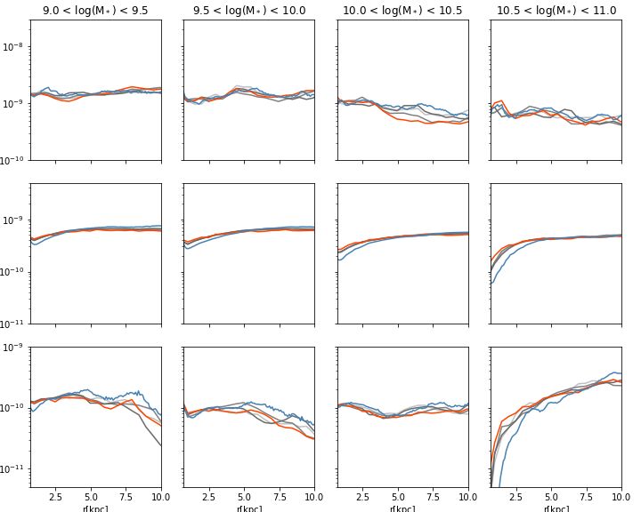
8 E. J. Nelson et al.

Table 1. Coefficients in the fit to the star forming main sequence in the TNG50 Table 2. Scatter in the star forming main sequence in 3D-
simulation versus observations from the 3D-HST survey both original v4.1.5 HST/Prospectorversus TNG50. This is measured in bins of stellar mass
and updated with Prospector. log ( ) = + log ( ∗ ) + log ( ∗ ) 2 with a width 0.5dex including observational uncertainties on both the obser-
 vations and simulations. (See §4.2 for more details.)
 data/sim a b c
 mass bins 3D-HST/Prospector TNG50 ratio
 3D-HST/Prospector -22.13 3.74 -0.146
 TNG50 -20.46 3.38 -0.127 9 < log(M∗ ) < 9.5 0.41 0.33 0.81
 3D-HST/orig -37.48 6.87 -0.302 9.5 < log(M∗ ) < 10 0.38 0.33 0.88
 Illustris/orig -14.21 2.08 -0.060 10 < log(M∗ ) < 10.5 0.45 0.32 0.72
 10.5 < log(M∗ ) < 11 0.57 0.33 0.58

0.1 dex uncertainty in this comparison due to aperture effects and the
timescale on which the SFR is measured, as described in Donnari mass in this Section: see Fig. 2. However, investigating the shape
et al. (2019). of this distribution requires properly accounting for observational
 Let us not lose sight of the main point, however: the SFMS in the uncertainties. Prospector returns a probability density function
TNG50 simulation and observations from 3D-HST are in remarkable (PDF) for each parameter it fits. In each bin, we sum the PDFs of
agreement. This is surprising given the longstanding 0.1−1 dex offset SFR normalized to the main sequence fit then normalize the overall
between the SFMSs in observations and simulations at = 1 − 2 (e.g distribution to have an area of 1. To make the distribution from sim-
Torrey et al. 2014; Sparre et al. 2015; Somerville & Davé 2015; Davé ulations more directly comparable, as mentioned in Section 3.2, we
et al. 2016; Donnari et al. 2019). So what changed? Let us first con- assign an observed PDF to each SFR in the simulation by drawing
sider the simulations. Illustris and TNG50 main sequences are shown randomly from the observed galaxies with similar masses and SFRs
in Fig. 1: light orange vs. yellow curves. There is little change going (as the width of the PDF is dependent on these quantities). We then
from Illustris to TNG50 at ∼ 1; the slope and normalization of the sum the TNG50 PDFs in the same way as the observed ones. In other
main sequence have remained similar. Turning to the observations, words we add observational uncertainties to the simulated SFRs so
the star forming main sequence from the original 3D-HST catalogs that the scatter is directly comparable.
(v4.1.5; Whitaker et al. 2014; Skelton et al. 2014) as well as a litera- Figure 2 (top row) shows this comparison – the distribution of
ture compilation (Speagle et al. 2014) are also shown. The normaliza- simulated and observed galaxies around the main sequence in bins
tion of the main sequence at ∼ 1 has decreased by 0.2−0.5 dex when of stellar mass. We remind the reader that observed and simulated
using the Prospector Bayesian inference framework to determine galaxies with very low SFRs ( double < 20 Hubble ( )) are not con-
stellar population parameters compared to previous determinations. sidered in this analysis. At all masses, the TNG main sequence is
The offset is minimized when adopting a non-parametric star for- narrower than the observations. That is, there is less scatter in the
mation history in the Bayesian inference framework, coupled with SFRs of the simulated galaxies than there is amongst the observed
accounting for infrared emission due to dust heated by older stellar galaxies. We note that we use the instantaneous SFR in the simula-
populations and supermassive black holes rather than star formation tions and the SFR averaged over 30Myr in observations. The scatter
(see Leja et al. 2019, for more information). Thus the long-standing of the main sequence measured from instantaneous SFRs will be
0.1 − 1 dex offset between the SFMS in observations and simulations larger than those averaged over longer timescales (e.g. Caplar & Tac-
at ∼ 1 disappears in this work not due to changes in the simulations chella 2019; Donnari et al. 2019; Tacchella et al. 2020) so likely the
but rather to changes in the stellar population parameters inferred difference in the scatter is even larger than we see here. This is less
from observations. Values for the coefficients in the ∼ 1 main dramatic below log(M∗ ) = 10 and more dramatic above. We quantify
sequence fit (equation above) are listed in Table 1. this difference in width by computing the width of the region that
 As shown in Torrey et al. (2014), the star forming main sequence contains 68% of the distribution. These values are listed in table 2.
in simulations is fairly insensitive to the nature of the feedback pre- For 9 < log(M∗ ) < 10, we find the simulations are 80-90% the width
scription. The integrated main sequence is thus not a particularly of observations. For 10 < log(M∗ ) < 10.5, the difference grows to
discerning validation of a simulation’s feedback model. As we will 70%; for 10.5 < log(M∗ ) < 11. to 60%.
show in the next section, this is not the case when looking at the The distribution is more skewed toward low SFRs in observations.
resolved properties of star formation across the main sequence. Fur- While in TNG50, the distributions are self-similar at all masses,
thermore, Leja et al. (2015) showed that earlier measurements of in observations they become more skewed toward high masses.
the star forming main sequence and the evolution of the stellar mass We quantify this by measuring the skew of the distributions of
function were not self consistent in observations: the SFMS dramat- the simulated vs. observed galaxies based on the ridgeline of the
ically overpredicted galaxy stellar mass growth. In the simulations distribution instead of the mean as in the standard definition. At
they are obviously self-consistent and hence unsurprising that they 10.5 < log(M∗ /M ) < 11, the observed distribution of SFR has a
could not simultaneously match both the observed main sequence skew of -2.3 while TNG50 has -1.5. The relative lack of low SFR
and mass function. With data that are self-consistent, the simulations galaxies in TNG50 is likely due to the prescriptions for AGN feed-
can match both as they are directly coupled. back in the simulation. Although we note from the observational side
 that SFRs of low-sSFR galaxies are the most model-dependent. On
 the simulation side, kinetic radio-mode AGN feedback is designed to
4.2 Width and outliers of the star forming main sequence
 very efficiently shut down star formation, while the thermal quasar-
Although the medians are nearly identical between TNG50 and mode is comparably inefficient (Weinberger et al. 2018). Within the
Prospector/3D-HST, the distribution of galaxies about these me- model, every black hole is in one of these two modes, with low-mass,
dians is not, even when accounting for observational uncertainties rapidly accreting black holes (living in low-mass or high redshift
in our treatment of the simulations. We look at the distribution of galaxies) being in the thermal mode. Once the accretion rate (rela-
the distance of galaxies from the median fit (ΔMS) in bins of stellar tive to the Eddington accretion limit) drops below a black hole mass

MNRAS 000, 1–15 (2021)

sSFR profiles in IllustrisTNG50 vs. 3D-HST 9

 3D-HST
 TNG50
 Illustris

 9.0 < log(M * ) < 9.5 9.5 < log(M * ) < 10.0 10.0 < log(M * ) < 10.5 10.5 < log(M * ) < 11.0
 3D-HST
 TNG
 starbursts

 2 0 2 2 0 2 2 0 2 2 0 2
 MS [log(M /yr)] MS [log(M /yr)] MS [log(M /yr)] MS [log(M /yr)]

Figure 2. Top: Distribution of simulated and observed galaxies around the main sequence in bins of stellar mass. We contrast the 3D-HST data (black), TNG50
simulation (light blue), and original Illustris simulation (purple). Although the width of these distributions are broadly consistent between the simulations and
observations at lower galaxy stellar mass, the simulated scatter is smaller than observed at high ( ★ > 1010 M ). Bottom: As above, except with the distribution
shifted to the ridgeline of the distribution of star formation rather than the median. With this shift applied, the shape of the distribution of galaxies above the main
sequence is similar between observations from 3D-HST/prospector and TNG50. The orange solid line shows the definition of “starbursts" used in §4 following
Rodighiero et al. (2011) and Sparre et al. (2015): > 2.5 above the main sequence.

dependent factor, the feedback mode switches to a kinetic mode, lead- 5 SSFR PROFILES IN TNG50 VS. 3D-HST
ing to an overly sharp decline, almost a jump, in sSFR as a function
 Here we compare the average radial profiles of sSFR in galaxies on,
of black hole mass as well as stellar mass and other properties of the
 above, and below the SFMS in observations from the 3D-HST sur-
simulated ∼ 0 galaxy population (Terrazas et al. 2020; Habouzit
 vey at ∼ 1 and the TNG50 magnetohydrodynamical cosmological
et al. 2019; Li et al. 2020; Habouzit et al. 2020). We speculate that,
 simulations. The derivation of the profiles is described in §2.4 for
similarly, ∼ 1 galaxies in TNG50 quickly quench whereas in the
 the observations and §3 for the simulations.
real universe massive galaxies seem more likely to tarry below the
 The sSFR profiles are a powerful diagnostic to understand where
main sequence before becoming fully quenched.
 the galaxies are growing. A flat sSFR profiles indicates that the stellar
 mass doubles at all radii with the same pace, implying a self-similar
 growth of the stellar mass density profile. An increasing sSFR toward
 Furthermore, at M∗ >1010 M above the main sequence an insuf- the outskirts implies that the galaxy grows stellar mass faster in the
ficient number of starbursts as compared to the real Universe was outskirts than in the center (galaxy grows in size), while a decreasing
noted in Illustris (Sparre et al. 2015). We quantify this by com- sSFR toward the outskirts is consistent with a galaxy that decreases
paring the fraction of star formation that occurs more than 2.5 its size.
above the main sequence in 3D-HST and TNG50 (as in Rodighiero
et al. 2011; Sparre et al. 2015). We calculate this fraction based
on both ridgelines of the distributions. Our definition is shown in
 5.1 Inside-out Quenching
Fig. 2 (bottom row). At high masses, TNG50 has a ridgeline which
is ∼ 0.15 dex lower than observations despite the medians being the A key result of this paper is that star formation is quenched
same. We also use the scatter as a function of mass from TNG50 to from the inside-out, which in the simulations is caused directly
compute this for both observations and TNG50 because the scatter by AGN feedback. Figure 3 shows that below the main sequence
is significantly smaller in TNG50 than observations at high masses. at 10.5

10 E. J. Nelson et al.

Figure 3. Top row: stacks of sSFR in TNG50 at random orientations. Bottom: specific star-formation rate (sSFR) radial profiles of massive galaxies, with
1010.5 < ★ /M < 1011 at ∼ 1. We contrast profiles inferred from observations with 3D-HST (dashed cuves) against the outcome of the TNG50
hydrodynamical simulation (solid curves), as a function of offset from the star-forming main sequence: galaxies which reside below (left), on (center), and above
(right). In all cases the TNG50 simulation broadly reproduces both the normalization and shape of the observed SFR radial profiles. A key result of this work is
that quenching galaxies (left) exhibit a clear central SFR suppression in the data as well as in TNG50. This supports the scenario of inside-out quenching, which
in TNG50 arises due to a central, short time-scale, ejective supermassive black hole feedback mechanism at low accretion rates. This is not the case with the
jet-inflated bubble black hole feedback model in Illustris as shown by the dash-dot purple line. The grey shaded region is inside the observed PSF.

lower spatial resolution). As shown through the comparison to the with cold clouds embedded in a hot, volume filling component, but
lower resolution version of TNG50, this is not a resolution effect but cells have a single, volume averaged density value and a pressure
due to the physics in the simulation. In Illustris, bubbles are blown according to an effective equation of state (Springel & Hernquist
at galactocentric distances of 50-100 kpc and consequently have a 2003). This means that AGN driven winds that interact with this
hard time propagating back into the denser gas to affect the center medium impact the entire mass budget, while a situation where the
of the galaxy. Hence the sSFR profiles in Illustris are not centrally wind propagates in low density channels while cold clouds continue
suppressed. In TNG50 on the other hand, both kinetic and thermal forming stars (e.g. Dugan et al. 2017) is not possible within the
feedback are done on the gas immediately surrounding the black IllustrisTNG model. It is possible that the effect of AGN winds would
hole, suppressing star formation from the inside-out. differ with a more realistically modeled ISM – a scenario testable
 with future simulations.
 In quantitative detail there remain small differences between the
observed and TNG50 sSFR profiles at high masses (i.e. log M∗ > In general the TNG AGN feedback model produces sSFR profiles
10.5) below the main sequence. While the sSFR profiles agree at the which are in better agreement with observations than the original
centers, for 2 < < 4 kpc TNG50 is about a factor of two higher Illustris simulation. The TNG black hole feedback model introduces
than observations. This implies that the central suppression of SFR powerful kicks when a black hole reaches a certain mass (Weinberger
does not extend to sufficiently large radii as seen in the data. This et al. 2017; Nelson et al. 2019b). These kicks evacuate gas from the
could be related to the modeling of the interstellar medium in this very center of the galaxy (Zinger et al. 2020), introducing enough
simulation: in particular, there is no explicit multi-phase medium feedback energy to gravitationally unbind gas from the galaxy. As

MNRAS 000, 1–15 (2021)

sSFR profiles in IllustrisTNG50 vs. 3D-HST 11

 9.0 < log(M * ) < 9.5 9.5 < log(M * ) < 10.0 10.0 < log(M * ) < 10.5 10.5 < log(M * ) < 11.0
 10 8
 above
 sSFR [yr 1]

 10 9
 3D-HST
 TNG50
 TNG50-2
 10 10 Illustris

 main sequence
 10 9
 sSFR [yr 1]

 3D-HST
 10 10 TNG50
 TNG50-2
 Illustris

 below
 10 10
 sSFR [yr 1]

 3D-HST
 TNG50
 10 11 TNG50-2
 Illustris
 2.5 5.0 7.5 10.0 2.5 5.0 7.5 10.0 2.5 5.0 7.5 10.0 2.5 5.0 7.5 10.0
 r [kpc] r [kpc] r [kpc] r [kpc]

Figure 4. sSFR profiles of ∼ 1 galaxies across the star forming main sequence – comparison between observations and TNG50, the original Illustris simulation,
and a lower resolution version of TNG50 with resolution more similar to that of Illustris (TNG50-2). Profiles are cut off when their signal-to-noise ratio falls
below 1. We find that TNG50 is more consistent with observations than the original Illustris simulation and that this is not primarily due to resolution effects.
The grey shaded region is inside the observed PSF.

described in Terrazas et al. (2020), these galaxies are likely in the 5.2 Flat sSFR profiles across the star-forming main sequence
process of unbinding their gas starting from the very central regions
and eventually expanding its effect to larger radii. Notably the origi- Average specific star formation rate (sSFR) profiles of galaxies on,
nal Illustris simulation, with its rather different physical mechanism above, and below the star forming main sequence in observations and
for AGN feedback at low accretion rates, based on jet-inflated bub- simulations are shown in Fig. 5. The main takeaway is that the sSFR
bles heating the ICM at distances of tens of kpc or more from the profiles across the main sequence in TNG50 are remarkably similar
galaxy, does not reproduce the central SFR profile suppression seen to those in observations. With few exceptions, at all masses and radii
in data. This different manifestation between the two feedback models the observed and simulated sSFR profiles lie within 0.3 dex (a factor
is clearly constrained by the observations. In summary, our findings of two) of each other.
support two key ideas: (i) in reality, massive galaxies quench from This agreement is surprising; it did not have to turn out this way.
the inside-out possibly due to locally acting AGN feedback, while (ii) The consistency shows that the distribution of dense gas and the
in the TNG simulations, the details of how supermassive black hole conversion of gas into stars are roughly correct in the simulation,
feedback are implemented and, in particular, how this feedback en- at least relative to the existing stellar mass. This means that the
ergy physically affects, heats, and redistributes gas appears to zeroth physical TNG50 model governing how galaxies grow in size and
order consistent with constraints from the observed star formation build their structures across the SFMS yield high fidelity predictions.
rate radial profiles on scales of a kiloparsec. The distribution of cold gas is set by the spatially dependent interplay
 between gas inflows, outflows, and star formation. The accretion of
 gas onto the galaxies is driven by gravity (a model about which there is

 MNRAS 000, 1–15 (2021)

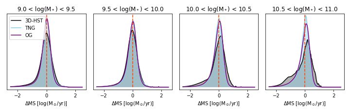
12 E. J. Nelson et al.

 9.0 < log(M * ) < 9.5 9.5 < log(M * ) < 10.0 10.0 < log(M * ) < 10.5 10.5 < log(M * ) < 11.0
 10 8
 above
 sSFR [yr 1]

 10 9

 3D-HST EW(H )
 3D-HST SED
 10 10 TNG50

 main sequence
 10 9
 sSFR [yr 1]

 10 10 3D-HST EW(H )
 3D-HST SED
 TNG50

 below
 10 10
 sSFR [yr 1]

 3D-HST EW(H )
 10 11 3D-HST SED
 TNG50
 2.5 5.0 7.5 10.0 2.5 5.0 7.5 10.0 2.5 5.0 7.5 10.0 2.5 5.0 7.5 10.0
 r [kpc] r [kpc] r [kpc] r [kpc]

Figure 5. The average radial sSFR profiles of galaxies across the star forming main sequence are very similar between TNG50 and observations at 0.75 < < 1.5.
The top row is above the main sequence, middle is on, bottom is below. The magenta in the bottom right corresponds to the AGN correction described in §2.4,
note it makes little difference. The grey shaded region is inside the observed PSF.

less uncertainty than the others) and suppressed by feedback. TNG50 formation over past star formation that is consistent with the real
uses the Springel & Hernquist (2003) model for star formation. In Universe.
this model gas above a certain density threshold is converted to
stars stochastically. While this model is too simple on small scales Above the main sequence the sSFR profiles from TNG50 and 3D-
(e.g. Semenov et al. 2019), it appears that on kpc scales this model HST are fairly flat. Star formation is not primarily enhanced in the
produces results that are consistent with observations. center meaning that it is not primarily driven by central starbursts. In
 this regime, the match with observations improved from Illustris to
 TNG. In Illustris the profiles have somewhat of a negative gradient
 Feedback has significant effects in all parts of the baryon cycle: it while in TNG50 (and 3D-HST observations) they do not. This is
affects inflow rates and geometries (e.g. Nelson et al. 2015) and it not primarily a resolution effect as the profiles in TNG-LowRes are
determines the distribution of cold gas and hence where the galaxy fairly flat like those in TNG50. Instead this is likely a physical effect
can form stars. In TNG50 outflows driven by supernova feedback owing to the implementation of supernova feedback. As shown in
are launched from star forming gas with their energy given by the obsevations as well as in TNG50 (Förster Schreiber et al. 2019;
star formation rate. This result means that at 0.75 < < 1.5 and Nelson et al. 2019b), star formation driven winds are strongest above
9