SPINDOWN ELECTROMAGNETIC PULSAR - IOANNIS CONTOPOULOS RCFA, ACADEMY OF ATHENS
←
→
Page content transcription
If your browser does not render page correctly, please read the page content below
Electromagnetic Pulsar Spindown

         Ioannis Contopoulos
         RCfA, Academy of Athens
Abstract
We review the recent developments on the issue of electromagnetic
pulsar spindown of a misaligned rotator. We evaluate them based
on our experience from two idealized cases, that of an aligned
dipolar rotator, and that of a misaligned split-monopole rotator, and
thus obtain a different spindown expression.
We next incorporate the effect of magnetospheric particle
acceleration gaps. We argue that near the death line aligned
rotators spin down much slower than orthogonal ones. We test this
hypothesis through a Monte Carlo fit of the P-Pdot diagram without
invoking magnetic field decay. We predict that the older pulsar
population has preferentially smaller magnetic inclination angles and
braking index values n>3. Finally, we offer an observational test of
our hypothesis.
2The oblique pulsar magnetosphere: Spitkovsky 2006
“Modeling of the structure of the highly magnetized magnetospheres
of neutron stars requires solving for the self-consistent behavior of
plasma in strong fields, where field energy can dominate the energy
in the plasma. This is difficult to do with the standard numerical
methods for MHD which are forced to evolve plasma inertial terms
even when they are small compared to the field terms. In these
cases it is possible to reformulate the problem and instead of solving
for the plasma dynamics in strong fields, solve for the dynamics of
fields in the presence of conducting plasma. This is the approach of
force-free electrodynamics (FFE).”
Spitkovsky 2006 applied the finite-difference time-domain (FDTD)
numerical method commonly used in electrical engineering to solve
the FFE equations that describe the evolution of an initially dipolar
magnetosphere which begins to rotate obliquely. The strength of the
method is very low numerical dissipation, which is useful in the
study of the current sheets and consequent strong discontinuities
that develop in the magnetosphere.
3The oblique pulsar magnetosphere: Spitkovsky 2006
An important question is what is the electromagnetic luminosity of the
inclined rotator, since currently the vacuum formula
B*2 r*6 Ω *4
L vac = 3
sin 2
θ
6c
is commonly used to infer the magnetic field of pulsars.
Spitkovsky 2006 evolved an oblique dipolar magnetosphere for about
1.2 turns of the star (fig. 1). He claims that the solution very quickly
settles to a constant electromagnetic energy flux which depends on the
magnetic inclination (fig. 2), and he obtains the formula
B r Ω
2 6 4
L pulsar = * *
3
(*
1 + sin 2
θ)
4c
We will now try to reproduce this result from basic principles. We will
start with a short presentation of the aligned rotator case.
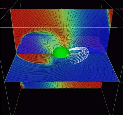
4The oblique pulsar magnetosphere: Spitkovsky 2006
Fig.1: Slices through the 60o magnetosphere. Shown are fieldlines in the horizontal
and vertical plane, color on the vertical place is the perpendicular field, on the
horizontal plane the toroidal field. A sample 3D flux tube is traced in white.
5The oblique pulsar magnetosphere: Spitkovsky 2006
Fig.2: Spindown luminosity in units of the aligned force-free luminosity (see text
below) as a function of inclination. Triangles represent simulation data.
1+sin2θ
6The aligned pulsar magnetosphere: CKF
Contopoulos, Kazanas & Fendt (1999, hereafter CKF) first obtained
the structure of the axisymmetric pulsar magnetosphere with a dipolar
stellar magnetic field (fig. 3). We showed that the asymptotic structure
is that of a magnetic split monopole: a certain amount of initially
dipolar magnetic flux Ψopen stretches out radialy to infinity in one
hemisphere, and returns to the star in the other hemisphere, forming a
current sheet discontinuity along the equator. Electromagnetic
spindown is due to the establishment of a poloidal electric current
distribution I=I(Ψ) which flows to infinity along open field lines and
returns to the star through an equatorial current sheet that joins at the
light cylinder with the separatrix between open and closed field lines.
CKF obtained Ψopen and the distribution I(Ψ) self consistently by
requiring that the solution be continuous and smooth at the light
cylinder.
The CKF solution has since been confirmed, improved and
generalized in Gruzinov 2005a, Contopoulos 2005, Timokhin 2005,
Komissarov 2005, McKinney 2005 and Spitkovsky 2006.
7The aligned pulsar magnetosphere: CKF
Fig.3: The axisymmetric pulsar magnetosphere (CKF). Thin lines correspond to Ψ intervals
of 0.1Ψdipole. Ψ=0 along the axis. The dotted line shows the separatrix Ψopen=1.23Ψdipole.
Distances are scaled to the light cylinder distance rlc=c/Ω*. A poloidal electric current flows
along the open field lines and returns along the equator and the separatrix between open
and closed field lines. No current flows in the closed line region.
8The aligned pulsar magnetosphere: CKF
The amount of initially dipolar field lines that stretches out radialy to
infinity is obtained numerically as
1/ 2
⎛3⎞
ΨopenCKF = 1.23Ψdipole ≈ ⎜ ⎟ Ψdipole
⎝2⎠
where
B*Ω*r*3
Ψdipole ≡
2c
is defined in the magnetostatic dipole problem as the amount of
dipolar flux that crosses a cylinder with radius equal to the light
cylinder radius. Interestingly enough, in the magnetostatic dipole
problem where field lines are required to open up beyond a distance
equal to the light cylinder radius (i.e. with a current sheet discontinuity
along the equator) the amount of open flux is found to be also closely
equal to the above value Ψopen!
9The aligned pulsar magnetosphere: CKF
The distribution I(Ψ) is found to be very close to that of the Michel 1991
split-monopole solution (fig. 4)
⎛ Ψ ⎞
I (Ψ ) ~ I Michel (Ψ ) ≡ Ψ ⎜ 2 − ⎟
⎜ Ψopen ⎟⎠
⎝
The electromagnetic spindown luminosity is thus obtained as
2 Ψ open
Ω 2 Ω *2 2 B *2 r*6 Ω *4
L aligned ≡
c
*
∫ I ( Ψ )d Ψ ≈
Ψ =0
3 c
Ψ open ≈
4 c 3
Note that, in the axisymmetric case, the spindown luminosity may be
obtained if one calculates the amount Ψopen of open field lines, since the
magnetosphere approaches asymptotically the Michel split-monopole
solution which depends only on Ψopen. As we will see next, this result is
also valid in the general case of an oblique rotator.
10The aligned split-monopole: Michel 1991
Fig.4: The axisymmetric split-monopole magnetosphere (Michel 1991). Thin lines
correspond to Ψ intervals of 0.1Ψopen. Ψ=0 along the axis. Distances are scaled to the light
cylinder distance rlc=c/Ω*. A poloidal electric current flows along the open field lines and
returns along the equator. In this idealized case, there is no closed line region.
11The oblique split-monopole: Bogovalov 1999
When studying the oblique rotator, it is natural to start from the
simplest case, that of an oblique split-monopole. Bogovalov 1991
showed that this problem is reduced to the problem of the
axisymmetric split-monopole rotator (fig.5). All properties of the cold
MHD plasma flows obtained for the axisymmetric rotator are the same
for the oblique rotator as well. In other words: as long as current sheet
discontinuities are present to guarantee magnetic flux conservation,
the direction of the magnetic field does not matter.
In particular, rotational losses of the oblique split-monopole rotator do
not depend on the inclination angle, but depend only on the amount
Ψopen of open field lines.
We may now derive an important conclusion about the oblique dipole
rotator which too, as we argued, becomes asymptotically split-
monopole-like: rotational losses of the oblique rotator depend
indirectly on the inclination angle through the amount of open field
lines Ψopen .
12The oblique split-monopole: Bogovalov 1999
Fig.5: The solution in the model with the oblique split-monopole magnetic field may be
obtained from the solution for the monopole magnetic field through the introduction of
current sheets and the appropriate changes of sign of the magnetic field.
Ω Ω, μ Ω, μ
μ μ μ
oblique rotator aligned split monopole monopole
current sheets
13The oblique dipole rotator: crude estimate
We have now come full circle and are in a position to estimate the
electromagnetic spindown luminosity as a function of the inclination
angle through an estimate of Ψopen . We may obtain a crude estimate
of Ψopen by calculating the amount of magnetic flux that crosses the
light cylinder and originates from an inclined magnetostatic dipole at
the origin, and rescale it by the CKF factor (3/2)1/2 (see fig. 6)
B*Ωr*3
Ψopen ~ 1.23 (0.4 + 0.6 cos θ )1/ 2
2c
This yields the following crude estimate of the spindown luminosity
B*2 Ω*4 r*6
L pulsar ~ 3
(0.4 + 0.6 cos θ )
4c
In particular, we see that Lpulsar(θ=90o) < Lpulsar(θ=0o), contrary to what
Gruzinov 2005b and Spikovsky 2006 obtain. This discrepancy will
need further analysis in order to be resolved.
14The oblique dipole rotator: crude estimate
Fig.6: The geometry used for a crude estimate of Ψopen. Note that Ψopen(θ=90o) is
smaller than Ψopen(θ=0o), hence we expect that Lpulsar(θ=90o) < Lpulsar(θ=0o), contrary
to what recent numerical simulations imply.
Ω open lines
μ
θ
Ψopen(θ=0o)=ΨopenCKF
Ψopen(θ=90o)~0.6ΨopenCKF
closed lines
light cylinder
15Magnetospheric gaps: Contopoulos & Spitkovsky 2006
The force-free MHD picture that we have been trying to develop
implies that charged particles are freely available in the
magnetosphere and support the required magnetospheric space
charges and electric currents. Those particles are produced in
magnetospheric potential gaps where a certain amount equal to about
Vgap~1013Volt of the total electromotive potential which develops along
the surface of the rotating star, V*~Ω*Ψopen/c, is “consumed” in order to
accelerate them. The effective remaining magnetospheric potential
(Ω* − Ω death )Ψopen
V=
c
is used to establish the force-free MHD solution. Here,
Ωdeath=Vgapc/Ψopen. Obviously, when Ω* drops below Ωdeath, electric
currents cannot be supported in the magnetosphere, pulsar emission
ceases, and the neutron star spins down as a vacuum oblique rotator.
16Magnetospheric gaps: Contopoulos & Spitkovsky 2006
We obtained an estimate of the spindown luminosity in the presence
of magnetospheric particle acceleration gaps, namely
⎛ ⎡ ⎤ ⎞
L pulsar ~
B*2 r*6 Ω *4 ⎜ α sin 2 θ + ⎢1 − Ω death ⎥ cos θ ⎟⎟
2
4c 3 ⎜ Ω*
⎝ ⎣ ⎦ ⎠
oblique rotator magnetospheric aligned rotator
contribution gap contribution contribution
We applied this expression with α=1 (our previous result suggests that
α may be equal to 0.4) to study how pulsars spin down (fig. 7), and
were able to reproduce the observed distribution of pulsars in the P-
Pdot diagram with the minimum number of assumptions possible,
through a simple Monte Carlo numerical experiment (figs. 8-10).
17Magnetospheric gaps: Contopoulos & Spitkovsky 2006
Fig.7: P-Pdot evolutionary diagram that shows the effect of the misalignment angle θ. Rectangular dots
indicate when pulsars reach Ωdeath and turn off. The dashed line represents the theoretical death line
which does not take into account the misalignment angle dependence. Oblique pulsars evolve faster
through the diagram.
θ=90ο
θ=30ο
θ=15ο
θ~0ο
18Magnetospheric gaps: Contopoulos & Spitkovsky 2006
Fig.8: Monte Carlo experiment using our new electromagnetic spindown expression.
Pulsars are injected with a distribution of polar magnetic field values around B*=1012G, and
initial periods at pulsar birth uniformly distributed between 10 msec and 0.2 sec.
19Magnetospheric gaps: Contopoulos & Spitkovsky 2006
Fig.9: The present day observed radio pulsar distribution for comparison with the result of
our Monte Carlo experiment. Data from ATNF pulsar catalog.
20Magnetospheric gaps: Contopoulos & Spitkovsky 2006
Fig.10: The distribution of |cosθ| in our Monte Carlo experiment. The dashed line represents the original
distribution injected with uniform random misalignment angle. The thick solid line corresponds to the
simulated pulsar distribution as a whole. The thin solid line corresponds to pulsars observed lying below
the theoretical death line.
21Magnetospheric gaps: Contopoulos & Spitkovsky 2006
Our main conclusions are:
1. The energy loss close to the pulsar death is smaller than what is
given by the standard dipolar spindown formula. This effect gives
a good fit between the theoretical and observed distributions of
pulsars near the death line, without invoking magnetic field decay.
2. The model may account for individual pulsars spinning down with
braking index n3. Such
high braking index values may be observable.
4. Pulsars near the death line may have preferentially smaller
inclination angles.
A preliminary look at the ATNF pulsar catalog data suggests that the
last point may have some observational support (fig. 11).
22Magnetospheric gaps: Contopoulos & Spitkovsky 2006
One possible measure of the inclination angle of a pulsar is its fractional
pulse width, or the ratio of the width of the pulse to the period of the
pulsar. If the radio beam size is independent of inclination, then we
would expect pulsars with smaller inclinations to be seen for a larger
fraction of the period than pulsars with large inclinations.
In order to test this hypothesis we took the available data for the pulse
width at 50% of the pulsar peak from the ATNF catalog (1375 pulsars
with W50%≠0). In order to be able to compare the fractional pulse width
for pulsars of different periods, we have to correct for the intrinsic size of
the pulsar beam. Therefore, the quantity that we relate to the degree of
alignment is Falign≡WP-1/2, where W is the measured pulse width. We plot
the observed pulsars as circles with the radius of the circle linearly
proportional to Falign.
A visual inspection of the plot shows that there is an excess of larger
pulse fractions for older pulsars, and in particular for pulsars beyond the
pulsar death line. This feature is particularly interesting and may serve
as an indication of alignment.
23Magnetospheric gaps: Contopoulos & Spitkovsky 2006
Fig.11: Distribution of alignment measure in the observed pulsar population. Each pulsar is
plotted as a circle with radius proportional to the quantity WP-1/2 using the pulse width W at
50% of the peak (see text). Data from ATNF pulsar catalogue.
24References
Bogovalov, S. 1999, A&A, 349, 1017
Contopoulos, I. Kazanas, D. & Fendt, C. 1999, ApJ, 511, 351 (CKF)
Contopoulos, I. 2005, A&A, 442, 579
Contopoulos, I. & Spitkovsky, A. 2006, ApJ, in press
Gruzinov, A. 2005a, Phys. Rev. Lett., 94, 021101
Gruzinov, A. 2005b, astro-ph/0502554
McKinney, J. C. 2006, MNRAS, 368, L30
Michel, F. C. 1991, Theory of Neutron Star Magnetospheres
(Chicago: Univ. Chicago Press)
Komissarov, S. S. 2006, MNRAS, 367, 19
Timokhin, A. N., 2006, MNRAS, in press
25You can also read