The Tesla Turbine Seminar
←
→
Page content transcription
If your browser does not render page correctly, please read the page content below
University of Ljubljana
                        Faculty of Mathematics and Physics

                                      Seminar
                      The Tesla Turbine

                           Matej Podergajs
                 Adviser: prof. dr. Rudolf Podgornik

                                    March 2011

                                        Abstract
   Treatment of a bladeless turbine designed by Nikola Tesla is given. First this invention,
which can also be used as a pump, is generally described. Then we consider a mathematical
model of Tesla turbine. Equations governing fluid flow in this model are simplified, but
are still non-linear. In order to solve them analitically, we neglect non-linear terms. Then
we oveview the numerical solution for previously simplified non-linear equations. Finally,
improvements of original design are presented and their possible use.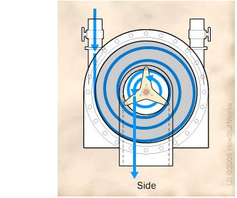
Contents
1 Introduction                                                                                      2

2 Historical background                                                                            2

3 Laminar flow between two parallel rotating discs - model               of Tesla turbine          4
  3.1 Statement of the problem . . . . . . . . . . . . . . . . . . .     . . . . . . . . . . . .   4
  3.2 Linearized treatment and asymptotic solution . . . . . . . .       . . . . . . . . . . . .   7
  3.3 Numerical solution of system of equations . . . . . . . . . .      . . . . . . . . . . . .   9

4 Applications                                                                                     10

5 Specific applications                                                                            11

6 Conclusion                                                                                       14

1    Introduction
Nikola Tesla was Serbian mechanical and electrical engineer and inventor, born in Croatia. He
is mostly known for his contributions in the field of electromagnetism, such as distribution of
electricity with alternating current and electric motor driven by alternating current. But he was
also interested in other areas. Among other things, he tried to improve water and wind turbines.
Tesla’s design of turbines is the topic of this seminar.

2    Historical background
In 1913 Nikola Tesla patented a turbine without blades, that uses a series of rotating discs to
convert energy of fluid flow to mechanical rotation, which can be used to perform useful work.
A Tesla turbine is made of a set of parallel discs with nozzles, through which gas or liquid enters
toward the edge of the discs (figure 1) [1]. Due to viscosity, momentum exchange takes place
between fluid and discs. As fluid slows down and adds energy to the discs, it spirals to the center
due to pressure and velocity, where exhaust is. As disks commence to rotate and their speed
increases, steam now travels in longer spiral paths because of larger centrifugal force. Fluid
used can be steam or a mixed fluid (products of combustion). Discs and washers, that separate
discs, are fitted on a sleeve, threaded at the end and nuts are used to hold thick end-plates
together. The sleeve has a hole, that fits tightly on the shaft. Discs are not rigidly joined, so
each disc can expand or contract (due to centrifugal force and varying temperature) freely. The
rotor is mounted in a casing, which is provided with two inlet nozzles, one for use in running
clockwise and other anticlockwise. Openings are cut out at the central portion of the discs and
these communicate directly with exhaust ports formed in the side of the casing. In a pump,
centrifugal force assists in expulsion of fluid. On the contrary, in a turbine centrifugal force
opposes fluid flow that moves toward center.
    In 1922 Tesla made some modifications (figure 2) [2]. In new design there are two heavier end-
plates, which are tapered toward the periphery for the purpose of reducing maximum centrifugal
stress. Inside discs are tapered in the same way or flat. Each plate has circular exhaust openings
3 and washers 5, like spokes of a wheel, that keep discs apart in the center. For peripheral spacing
tight-fitting studs 6 are used on every second plate. This can also be achieved with protuberances
which are raised in the plates by blows or pressure.

                                                 2
Figure 1: Original sketch of the Tesla turbine (left) [1]. Fluid enters through inlets 24 through
nozzles 25 and comes in contact with discs 13. It exists through openings 14 and continues to
outlets 20. If we need a pump, fluid flow must be reversed. Discs are held in place by spokes 15
and washers 17. Schematic presentation of fluid path (right) [3].
Tesla intended to use his turbine to propel aircraft, in geothermal power plants, in cars
instead of pistons, for vacuum pumps, for compressing air and liquifying gases. His turbine
(figure 3), with discs 22.5 cm in diameter and entire rotor 5 cm thick, used steam as propulsive
fluid and developed 110 horse power.
In general, spacing should be such that the entire mass of fluid, before leaving the rotor,
is accelerated to a nearly uniform velocity, not much below that of periphery of the discs. An
efficient turbine requires small inter-disc spacing (0.4 mm in a steam powered type). Discs must
be maximally thin to prevent drag and turbulence at the edges. But metallurgical technology in
Tesla’s time was unable to produce discs of sufficient rigidity to prevent warping at high rotation
rates. This drawback is probably the main reason why the turbine was never commercially
interesting [4].
If we connect motor to the shaft, we get a pump (figure 4). Fluid enters at the center and
starts to move tangentially due to viscosity. Now centrifugal force acts on the fluid also, which
results in spiral outward movement.
Efficiency decreases with increasing load on shaft. If we have a heavy load, the spiral path of
fluid is shorter than with light load. With heavy loads, average fluid velocity is smaller, which
results in smaller centrifugal force acting on the fluid. So fluid’s radial distance from center
exhaust, as it moves from edges to the center, decreases faster than in case of a light load. If the
path is shorter, less momentum is transfered from the fluid to the discs. This increases shear
losses and lowers efficiency. Performance of the turbine is strongly dependent on efficiency of
nozzles and the nozzle-rotor interaction. Performance of the pump is also strongly dependent on
interaction of fluid leaving the rotor with that in the volute and on the efficiency of the volute.
While rotor efficiencies can be very high, there are inherent losses in fluid flows entering and
exiting the rotor, so overall efficiency is much less than might be expected from consideration
of flow in the rotor [6]. Tesla claimed, that a steam version of his turbine would achieve around
90% efficiency. In the 1950s, Warren Rice built and measured efficiency of a turbine similar to
Tesla’s, he used air as working fluid. He achieved efficiency between 36% and 41% [4, 7]. Tesla-
type pumps with good rotor design have efficiencies in the range of 40 to 60% [6]. Contemporary
steam turbines can achieve efficiencies well above 50% [4]. Keep in mind, that turbine efficiency
3Figure 2: Modification of the Tesla turbine [2].
Figure 3: Tesla turbine that used steam as motive agent and developed 110 horse power [4].
is different from cycle efficiency using that turbine.
3 Laminar flow between two parallel rotating discs - model
of Tesla turbine
3.1 Statement of the problem
We use cylindrical polar coordinates r, φ, z. Imagine two discs, one at z = −d other at z = d,
both rotating about the z axis with constant angular velocity ω. Each disc has a circular opening
centered at r = 0, where r is distance from z axis. We assume, that an incompressible viscous
fluid enters space between discs in radial direction through cylindrical surface (figure 5). Due
to viscosity, it starts to move tangentially and then centrifugal force starts to act on the fluid.
Resulting path of the fluid is spiral.
Flow of viscous incompressible fluids is described by Navier-Stokes equation [8]:
4Figure 4: Tesla pump (solid arrow) or compressor (dashed arrow). Each disk has a number of
central openings 6, solid portions between them form spokes 7 [5].
∂u
ρ + (u · ∇)u = ρf z − ∇p + η∇2 u. (1)
∂t
Here ρ is density, f z are external forces per unit mass of fluid, p is pressure, η dynamic viscosity
and u fluid velocity. In our problem we consider fluid flow that is: steady, incompressible,
viscous and axisymmetric. We also neglect external forces, in this case force of gravity. Thus
simplified Navier-Stokes equation can be written in system of cylindrical polar coordinates fixed
in space (where u = (u, v, w)) in the following way [9]:
∂u v 2
2
∂ u ∂2u
∂u 1 ∂p ∂ u
u +w − = − +ν + + ,
∂r ∂z r ρ ∂r ∂z 2 ∂r r ∂r2
2
∂ v ∂2v
∂v ∂v uv ∂ v
u +w + = ν + + ,
∂r ∂z r ∂z 2 ∂r r ∂r2
2
∂ w 1 ∂w ∂ 2 w
∂w ∂w 1 ∂p η
u +w = − +ν + + , ν= . (2)
∂r ∂z ρ ∂z ∂z 2 r ∂r ∂r2 ρ
Equation of continuity is in this case
∂u u ∂w
+ + = 0. (3)
∂r r ∂z
If we assume, that variations of u = (u, v, w) with z are much more rapid than those with r or φ
[10, page 281] and that pressure difference normal to the discs is negligible [9], these equations
simplify to:
∂u ∂u v 2 1 dp ∂2u
u +w − = − +ν 2,
∂r ∂z r ρ dr ∂z
∂v ∂v uv ∂2v
u +w + = ν 2, (4)
∂r ∂z r ∂z
∂u u ∂w
+ + = 0. (5)
∂r r ∂z
5Figure 5: Schematic diagram of flow between two rotating discs, where ri is radius of entrance
hole, 2d distance between discs and ω constant angular velocity of the discs [9].
It is convenient to introduce tangential velocity V relative to the discs
V = v − rω, (6)
so simplified flow equations (4) take the form:
∂u ∂u V 2 + 2V rω + r2 ω 2 1 dp ∂2u
u +w − = − +ν 2,
∂r ∂z r ρ dr ∂z
2
∂V ∂V u (V + rω) ∂ V
u +ω +w + = ν 2. (7)
∂r ∂z r ∂z
Terms −2V ω and 2uω represent Coriolis force per unit mass and term −rω 2 represents centrifu-
gal force per unit mass of fluid. Boundary conditions at the surface of the discs are:
u(r, z = ±d) = 0,
V (r, z = ±d) = 0,
w(r, z = ±d) = 0. (8)
We must prescribe velocity distribution in the entrance cross section to solve this problem:
u(ri , z) = u0 ,
V (ri , z) = −rω. (9)
63.2 Linearized treatment and asymptotic solution
If we omit quadratic terms in u, V and w, equations (7) reduce to
ν ∂2u 1 dp
+ 2V = − rω, (10)
ω ∂z 2 ρω dr
ν ∂2V
u = . (11)
2ω ∂z 2
Right side of equation (10) does not depend upon z. Velocity component w does not appear
in these equations, so first we must solve them and then obtain w from equation (5). Only
expression with derivatives with respect to r is
1 dp
− rω = F (r), (12)
ρω dr
so equations can be solved for each value of r independently. This expression will be represented
in solution for u and V as a factor, that depends only on r. This factor is determined from
condition, that mass flow between discs is constant for every surface with constant r. After
elimination of u, we obtain from equations (10) and (11)
∂4V
+ 4α4 V = 2α4 F (r), (13)
∂z 4
p
where α = ω/ν. The most general solution, that satisfies symmetry conditions at z = 0 is
F (r)
,
V = A1 sinh(αz) sin(αz) + A2 cosh(αz) cos(αz) + (14)
2
where A1 and A2 do not depend upon z. They can be determined from boundary conditions
(8) and equation (11):
sinh(αd) sin(αd) F (r)B1
A1 = −F (r) =− ,
cosh(2αd) + cos(2αd) 2
cosh(αd) cos(αd) F (r)B2
A2 = −F (r) =− , (15)
cosh(2αd) + cos(2αd) 2
where we introduced B1 and B2 .
Volume flow of fluid Q through a surface with constant r extended between discs is
+d +d +d
∂2V
Z Z
πr πr ∂V
Q = 2πr udz = dz = 2 =
−d α2 −d ∂z 2 α ∂z −d
πrF (r) sinh(2αd) − sin(2αd)
− . (16)
α cosh(2αd) + cos(2αd)
Now function F (r) can be obtained:
αQ cosh(2αd) + cos(2αd) 2q
F (r) = − =− , (17)
πr sinh(2αd) − sin(2αd) r
where we defined quantity q. Finally, velocity components can be expressed in terms of volume
flow:
7q
V = [B1 sinh(αz) sin(αz) + B2 cosh(αz) cos(αz) − 1] , (18)
r
q
u = [B1 cosh(αz) cos(αz) − B2 sinh(αz) sin(αz)] . (19)
r
If we insert these equations in continuity equation (3), we see that w = 0. Velocities in the
middle plane between discs are: V (r, z = 0) = (B2 − 1)q/r, and u(r, z = 0) = B1 q/r. Because
we neglected quadratic terms in velocity, these solutions are good at large radii and can be
viewed as asymptotic solutions for actual non-linear system of equations (5) and (7).
Figure 6 shows radial velocity component u as dimensionless quantity. For small values of
αd profiles have a near parabolic shape with maximum velocity in the middle (z = 0). For
αd = π/2 the profile is flat in the middle, for higher values of αd the flow is more concentrated
in vicinity of the discs.
Figure 6: Radial velocity component u (as dimensionless quantity) for different values of αd as
function of z/d for q/r = 1 [9].
Relative tangential velocity V (in dimensionless form) is shown in figure 7. For small values
of αd it also has a parabolic shape, but as αd increases, slope in the neighbourhood of the discs
becomes steeper and relative velocity V in middle plane approaches −1. This is understandable,
because higher values of αd mean larger inter-disc spacing at same angular speed with the same
fluid, or higher angular speed and fluid with smaller kinematic viscosity ν at same inter-disc
spacing.
Results for large values of αd should be viewed cautiosly. In this regime u may become
negative in the middle, which means we have radial outflow near discs with radial inflow in the
middle. It would require a rather special arrangement for such flow to take place.
Dimensionless parameter αd is of importance, since it determines the character of u and V .
This parameter does not depend upon radius r or volume flow Q. If we want to use a fluid with
small kinematic viscosity and/or have high angular velocity of discs, distance between discs must
be small.
Torque required at the shaft of the rotor can be computed from frictional forces acting on
inner side of two disks:
8Figure 7: Relative tangential velocity V (as dimensionless quantity) for different values of αd as
function of z/d for q/r = 1 [9].
Z r
∂V
M = 2 · 2πη r2 dr. (20)
ri ∂z z=d
3.3 Numerical solution of system of equations
In previous subsection we assumed, that velocity components are small. This is not valid in
vicinity of the entrance, especially for tangential velocity relative to the discs. And linearization
changes flow equations to such degree (all derivatives of velocity components with respect to r
vanish), that boundary conditions at the inlet cannot be satisfied.
For numerical computations, cartesian coordinate system was used. Its origin lies in entrance
cross section at the lower disk and x axis is on the lower disk. Now we have
x = r − ri ,
y = z + d.
We introduce dimensionless variables in the system of differential equations (5) and (7):
u x
u = , x = , r = 1 + x,
ri ω ri
r r
V ω ω
V = , y=y , d=d ,
ri ω ν ν
w
w = √ .
νω
Exit cross section does not play a special role in this procedure, so each value of r can be
considered as outer radius of the rotor. We will omit description of numerical procedure, which
is given in [9], and go straight to results. Assuming that velocity at the entrance u0 is constant
9and V0 = −1 because of equation (6), solutions for u0 = 1.0, 0.5, 0.25, 0.1 and d = 0.5, 1.0, 1.5, 2
are plotted in [9]. Here is only one of them (figure 8 and figure 9).
Figure 8: Radial velocity u for u0 = 1.0 and d = 1.5 versus z/d with r/ri as parameter [9].
These and other solutions in [9] have the following in common: at the wall inlet velocities
u0 and V0 are immediately reduced to zero due to boundary conditions. Reduction of radial
velocities at the wall causes velocities in the middle to increase. Therefore in vicinity of the inlet
radial velocity in the middle between discs overshoots radial velocity u0 . Effect decreases with
increasing r, because available cross section increases and velocity profile finally approaches the
form given by linearized theory.
Average tangential velocity is directly connected with torque M that acts on discs due to
viscous effects and thus with work required to drive the pump.
Efficiency η is in [9] defined by
p
η=Q , (21)
Mω
where Q = 2πri ·2u0 d is volume flow of fluid entering at ri and p is pressure. Pressure distribution
is computed from the function F (r). Torque M can be obtained from equation (20). In [9] M ,
p and η versus r/ri are plotted for chosen values of u0 and d. Here we have one of these plots
for η (figure 10). We see, that efficiency decreases with increasing u0 , which is proportional to
incoming volume flow.
4 Applications
Prior to 2006, Tesla turbine was not commercially used. On the other hand, Tesla pump has
been commercially available since 1982. It is used to pump fluids that are abrasive, viscous,
contain solids or are difficult to handle with other pumps. The concept of Tesla turbine is used
as a blood pump and gave good results. Research in this field still continues. In 2010, a patent
was issued for a wind turbine based on Tesla design.
In Tesla’s time efficiency of classic turbines was low, because aerodynamic theory needed to
construct effective blades did not exist and quality of materials for blades was low. That limited
10Figure 9: Relative tangential velocity V for u0 = 1.0 and d = 1.5 versus z/d with r/ri as
parameter [9].
operating speeds and temperatures. Its other drawbacks are shear losses and flow restrictions.
But that can be an advantage when flow rates are low. Tesla’s design can also be used, when small
turbine is needed. Efficiency is maximized, when boundary layer thickness is approximately equal
to inter-disc spacing. So at higher flow rates, we need more discs, which means larger turbine.
Because thickness of boundary layer depends on viscosity and pressure, various fluids cannot
be used as motive agents in the same turbine design. Discs have to be as thin as possible, to
prevent turbulence at disc edges.
5 Specific applications
After two original designs patented by Tesla, inventors tried to improve them. In U.S. patent
4655679 from 1987, planar carbonized composite discs were proposed instead of metal ones.
These discs can sustain considerable mechanical and thermal stress and are more resistant than
multi-bladed rotors made from the same material. At higher temperatures of incoming gases,
higher efficiencies are obtainable. Turbines of this design can operate at temperatures above
1000◦ C. Disks are separated by rings 32, and have circular exhaust openings 33 (figure 11) [11].
Electronically controled guidewall 55 is used to direct gas to the entire rotor or only a part of it,
when gas flow varies. This maintains flow between two discs within desired range, so efficiency
is not compromised. Vanes 50 divide inflowing gasses into channels 51 with as little turbulence
as possible. Turbulence is minimized because gasses are not permitted to expand significantly
prior to their entry into the rotor and because inlet channels 51 act to smoothly divide gasses
into individual flow paths in agreement with spaces between discs. This design can also be used
as a pump, for example in cars to deliver compressed air to carburation system.
In U.S. patent 0053909 from 2003, there are airfoils between discs. Airfoils are placed in
such manner, that they guide fluid flow toward central opening 5 that acts as exhaust (figure
12). Fluid flows through nozzles, that direct fluid between discs and on leading edges of airfoils,
as arrow 3 shows [12]. Momentum is exchanged through 3 mechanisms: fluid flow strikes the
11Figure 10: Efficiency η versus r/ri for d = 1.5 with u0 as parameter [9].
leading surface of airfoils, fluid flow around airfoils produces lift on them and viscous interaction
between disc surface and fluid. They all contribute to rotational output, for lift on an airfoil is
perpendicular to freestream velocity [8]. Only some airfoils extend from outer edge of the disc
to the outer edge of exhaust outlet, because we have to have enough opening area for exhaust
gasses. Shaft can be connected to one of the outer discs, that does not have a central opening,
and exhaust gasses leave the turbine from space between this and adjacent disc. Such turbines
can be made of composite materials. It has only few moving parts (cheaper manufacture)
and lubrication is required only for shaft bearings (environmentaly friedly). Because discs are
connected through airfoil shaped parts, they are more resistant to deformations at higher angular
speeds. It is intended for use in turbine engines.
U.S. Patent 7695242 was issued in 2010 for wind turbine intended for generation of electric
power, shown in figure 13, and can also be used in geothermal applications. It consists of
parallel discs 1 connected to a shaft by spokes 5. Discs are in periphery separated by spacers
3, which have an airfoil shape. If the radius of discs is R, spacers should be positioned at
least at a distance 0.95R from center of the discs. Here airfoil sections occupy smaller part of
discs, so majority of their surface can be used for boundary layer effects, such as in original
Tesla’s designs. Spacers are angled toward the axis of rotation, where exhaust 6 is, and they
guide the fluid towards exhaust. When fluid enters the rotor, it hits spacers. This generates
drag and lift on them, hence energy of fluid is more efficiently converted into electrical energy.
Rotor rotates also because of viscous effects between discs and entering fluid [13]. Near center,
spokes serve as spacers. Both kinds of spacers provide considerable rigidity of the discs. If
turbine is used for harnessing wind power, its outlet channel 13 is longer, with at least one flat
surface. This automatically aligns the apparatus with wind direction. Housing has vanes or
louvres 25 to regulate flow into the turbine. This turbine can be mounted on a tower shorter
in comparison to towers for conventional turbines, because entire rotor is closed in a housing.
This also prevents injury to birds and bats. Generator equipment can be located at tower base,
so routine maintenance is simpler and cheaper. If it is used in geothermal power plants, it can
operate on relatively cool fluids. In contrast, conventional turbines would require fluids hot
enough to produce superheated steam. Due to airfoil spacers, it is efficient in wider range of
flow rates, than turbines with plane discs but no airfoil spacers. Therefore it is more suitable
for harnessing wind power, whose flow is quite variable.
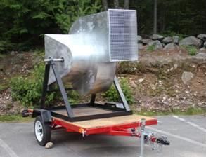
Based on this patent, Solar Aero company from New Hampshire constructed a turbine (figure
12Figure 11: Design with carbonized composite discs in the patent from 1987 [11].
14), for which they claim it can generate power at a cost comparable to power plants using coal
[14]. Turbine is compact and its only movable part is rotor with shaft. Total operating cost over
the lifetime of the unit is estimated at about 0.12$/kWh, which is, in USA, comparable to other
sources. Production licenses will be available as soon as characterization of the prototype wind
turbine is completed.
In 1999 a multiple disc centrifugal pump was analyzed as a blood pump for use in cardiac
assistance or as a bridge to transplant device. The original configuration consisted of 6 parallel
discs with 0.04 cm spacing between discs. This pump suffered from degradation of flow with
increasing afterload. Next, different configurations were analyzed. They included 4, 5 and 6
discs each with spacing of 0.4, 0.5 and 0.6 cm. Flow rates were examined for variations in blood
pressure and for motor speeds of 1250, 1500, and 1750 rpm. Results indicated that a 5 disk
configuration with a 0.4 cm spacing produced optimal flow results with minimal degradation
at higher afterloads. Levels of blood damage was below those of many other centrifugal blood
pump designs [15].
A small scale Tesla turbine prototype has been designed and built at Vanderbilt University
(Tennessee, USA). It is intended for a program, that is focused on providing electrical power
(0-100W) for foot soldiers’ on-board systems with an energy density greater than that of current
batteries [16]. High pressure gas resulting from an exothermic chemical reaction is directed
through a nozzle (or nozzles) and subsequently converted into shaft power via viscous drag
between closely spaced co-rotating discs. Shaft power is converted to electrical power through a
brushless generator.
13Figure 12: Design with airfoils between discs in the patent from 2003 [12].
Figure 13: Design with airfoils between discs in the patent from 2010 [13].
6 Conclusion
We summarized the development of Tesla’s turbine design. Due to technology limitations, it
has not seen widespread use in time of its conception. During last three decades, design has
Figure 14: Wind turbine from Solar Aero Company [14].
14been used in some areas, but not widely. If last issued patents live up to expectations of their
inventors, things may change.
References
[1] N. Tesla, D. H. Childress, The Fantastic Inventions of Nikola Tesla (Adventures Unlimited
Press, Stelle, Illinois, 1993).
[2] http://www.rexresearch.com/teslatur/turbine2.htm (2.1.2011).
[3] http://auto.howstuffworks.com/tesla-turbine3.htm (21.3.2011).
[4] http://en.wikipedia.org/wiki/Tesla_turbine (19.12.2010).
[5] http://www.rexresearch.com/teslatur/teslatur.htm (1.1.2011).
[6] http://www.rexresearch.com/teslatur/turbine3.htm (3.1.2011).
[7] http://www.teslaengine.org/images/teba15p17.pdf (3.1.2011).
[8] R. Podgornik, Mehanika kontinuov, study material, http://www-f1.ijs.si/ rudi/lectures/mk-
1.9.pdf (22. 12. 2010).
[9] M. C. Breiter, K. Pohlhausen, Laminar flow between two parallel rotating disks (Applied
Mathematics Research Branch, United States Air Force, 1962).
[10] D. J. Acheson, Elementary fluid dynamics (Oxford University Press, 1996).
[11] http://www.patentgenius.com/patent/4655679.html (3.1.2011).
[12] http://ip.com/patapp/US20030053909 (4.1.2011).
[13] http://www.scribd.com/doc/35806500/Us-7695242 (4.1.2011).
[14] http://www.physorg.com/news192426996.html (4.1.2011).
[15] http://onlinelibrary.wiley.com/doi/10.1046/j.1525-1594.1999.06403.x/abstract; jses-
sionid=705714B2EDC162724C4F42B8CBD08781.d03t02 (4.1.2011).
[16] http://www.vanderbilt.edu/dces/tesla.html (4.1.2011).
15You can also read