Three-dimensional segmentation and reconstruction of the retinal vasculature from spectral-domain optical coherence tomography
←
→
Page content transcription
If your browser does not render page correctly, please read the page content below
Three-dimensional segmentation and
                 reconstruction of the retinal
                 vasculature from spectral-domain
                 optical coherence tomography

                 Pedro Guimarães
                 Pedro Rodrigues
                 Dirce Celorico
                 Pedro Serranho
                 Rui Bernardes

Downloaded From: https://www.spiedigitallibrary.org/journals/Journal-of-Biomedical-Optics on 13 Jun 2022
Terms of Use: https://www.spiedigitallibrary.org/terms-of-use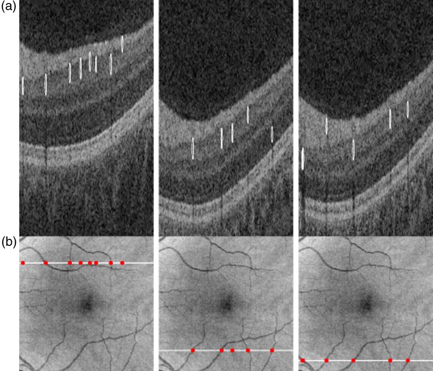
Journal of Biomedical Optics 20(1), 016006 (January 2015)

                Three-dimensional segmentation and reconstruction
                of the retinal vasculature from spectral-domain optical
                coherence tomography
                Pedro Guimarães,a,b Pedro Rodrigues,c,d Dirce Celorico,c Pedro Serranho,a,e,* and Rui Bernardesa
                a
                  University of Coimbra, Faculty of Medicine, Institute for Biomedical Imaging and Life Sciences, Azinhaga Santa Comba,
                3000-548 Coimbra, Portugal
                b
                  University of Padova, Department of Information Engineering, Via Gradenigo, 6/b, 35131 Padova, Italy
                c
                  Association for Innovation and Biomedical Research in Light and Image, Azinhaga Santa Comba, 3000-548 Coimbra, Portugal
                d
                  University of Coimbra, Institute of Systems and Robotics, Pinhal de Marrocos—Polo II, 3030 Coimbra, Portugal
                e
                  Universidade Aberta, Mathematics Section, Department of Science and Technology, Rua da Escola Politécnica 141-147,
                1269-001 Lisbon, Portugal

                              Abstract. We reconstruct the three-dimensional shape and location of the retinal vascular network from com-
                              mercial spectral-domain (SD) optical coherence tomography (OCT) data. The two-dimensional location of retinal
                              vascular network on the eye fundus is obtained through support vector machines classification of properly
                              defined fundus images from OCT data, taking advantage of the fact that on standard SD-OCT, the incident
                              light beam is absorbed by hemoglobin, creating a shadow on the OCT signal below each perfused vessel.
                              The depth-wise location of the vessel is obtained as the beginning of the shadow. The classification of cross-
                              overs and bifurcations within the vascular network is also addressed. We illustrate the feasibility of the method in
                              terms of vessel caliber estimation and the accuracy of bifurcations and crossovers classification. © 2015 Society of
                              Photo-Optical Instrumentation Engineers (SPIE) [DOI: 10.1117/1.JBO.20.1.016006]

                              Keywords: optical coherence tomography; vascular system; retina.
                              Paper 140421R received Jul. 1, 2014; accepted for publication Dec. 5, 2014; published online Jan. 7, 2015.

                1     Introduction                                                                 backscattering of low-coherence light, is now extensively
                The retina is regarded as a window to the cardiovascular system.                   described in the literature.12,13
                                                                                                       On standard spectral-domain OCT (SD-OCT) scans, the reti-
                Changes in the retinal microvasculature have been found to be
                                                                                                   nal blood vessels are not directly visible. Instead, two signatures
                related to several cardiovascular1–3 and cerebrovascular3–8 out-
                                                                                                   emerge in the OCT signal. One relates to the fact that hemoglo-
                comes, among other.9–11 These evidences make the automatic
                                                                                                   bin absorbs the infrared light. Consequently, backscattering at
                detection of retinal blood vessels a key step in this area of
                                                                                                   the structures below perfused vessels is highly attenuated.12,14,15
                research. The quantitative description of the detected retinal vas-
                                                                                                   This effect is well known and has been used to obtain the 2-D
                culature can be and has been used to establish the association                     vascular network from the 3-D OCT data.16–18 While this is a
                between retinal vascular properties and clinical and subclinical                   major advantage for 2-D segmentation due to the significant
                outcomes, thus providing tools to the clinician for an objective                   contrast on the retinal pigment epithelium (RPE), the 3-D seg-
                diagnosis.                                                                         mentation of the retinal vasculature requires additional informa-
                    Extensive work has been done in this field, mainly based on                    tion. The other signature is a diffuse hyper reflectivity on the
                two widely used ocular imaging modalities: color fundus pho-                       vessel itself.
                tography (CFP) and fluorescein angiography (FA). Vascular                              Approaches for 3-D retinal vasculature segmentation in the
                properties such as tortuosity or bifurcation angles computed                       literature are limited in number.19–21
                from these two-dimensional (2-D) fundus images have been                               In this work, we describe a fully automatic method for the
                associated with several diseases. However, the computation                         3-D segmentation of the vascular network of the human
                of such properties is incomplete due to the projection to a 2-                     retina from standard Cirrus HD-OCT (Carl Zeiss Meditec,
                D plane. A robust method to segment the human retinal vascular                     Dublin, CA, United States) data and the framework for its
                network in three-dimensions (3-D) would be a valuable tool and                     reconstruction.
                a significant leap forward to fully understanding the pathophysi-
                ology of several diseases.
                    Optical coherence tomography (OCT) is an imaging modal-                        2       Workflow and Background Work
                ity capable of noninvasively imaging the microstructure of tissue                  Following a preliminary study by our research group,22 the 3-D
                in vivo and in situ.12,13 Over time, it became an important tool                   OCT scan is projected to a 2-D ocular fundus reference image.
                in the diagnosis of ocular pathologic conditions. It has been                      Each pixel in this image translates into an A-scan on the OCT
                extensively used in clinical research and is becoming                              volume. This reference is then used to compute features that are
                common in the clinical practice. The principle, based on the                       able to discriminate each pixel into vessel or nonvessel groups.23
                                                                                                   The A-scans whose pixels were classified into the vessel group,

                *Address all correspondence to: Pedro Serranho, E-mail: serranho@uab.pt            0091-3286/2015/$25.00 © 2015 SPIE

                Journal of Biomedical Optics                                               016006-1                                         January 2015   •   Vol. 20(1)

Downloaded From: https://www.spiedigitallibrary.org/journals/Journal-of-Biomedical-Optics on 13 Jun 2022
Terms of Use: https://www.spiedigitallibrary.org/terms-of-use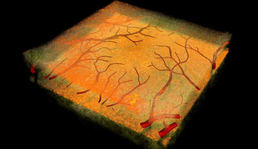
Guimarães et al.: Three-dimensional segmentation and reconstruction of the retinal vasculature. . .

                                     OCT 3-D               Layer                3-D/2-D             2-D Feature    2-D Supervised
                                      Scan              segmentation           Projection            extraction     classification

                                                                                                                        3-D              Vascular
                                                                                                                    Segmentation         network

                                                          Fig. 1 Flowchart representing the global workflow of the algorithm.

                i.e., A-scans that intersect blood vessels, are then processed to                  2.2     Ocular Fundus Reference Images
                determine the depth-wise location of the vessel. Figure 1 shows
                the global workflow of the algorithm and Fig. 2 shows a graphi-                    As noted, light absorption by hemoglobin is responsible for the
                                                                                                   decrease in light backscattering beneath perfused vessels. The
                cal depiction of the process.
                                                                                                   segmentation process herein takes advantage of this effect by
                    Throughout this paper, the following coordinate system for
                                                                                                   computing a set of 2-D fundus reference images from the 3-
                the OCT data will be used: x is the nasal-temporal direction, y is
                                                                                                   D OCT data (Fig. 2). A study was conducted to identify the fun-
                the superior-inferior direction, and z is the anterior-posterior
                                                                                                   dus reference images that provide the best discrimination
                direction (depth).
                                                                                                   between the vascular network and the background.26 Four
                                                                                                   potential reference images were evaluated:26 the mean value fun-
                                                                                                   dus (MVF), the expected value fundus (EVF), the error to local
                2.1     Retinal Layer Segmentation                                                 median (ELM), and the principal component fundus (PCF).
                The very first step consists of determining the depth coordinates                     The PCF image is computed through principal component
                of three interfaces: Z1 is the inner limiting membrane (ILM), Z2                   analysis (PCA) as the principal component of the MVF,
                is the junction between the inner and outer photoreceptor seg-                     EVF, and ELM images. The interfaces at coordinates Z2 and
                ments (IS/OS), and Z3 is the interface between the RPE and the                     Z3 are needed for this stage of the process. It was demonstrated
                choroid. These interfaces are typically the easiest ones to                        that the PCF image provides the greatest extension of the vas-
                                                                                                   cular network (equivalent to that achieved with CFP) and the
                identify.
                                                                                                   best contrast among the other fundus reference images.26
                    The retinal layer segmentation process itself will not be dis-
                cussed here in great detail. On one hand, it does not greatly
                affect the quality of the results of the final 3-D vascular segmen-
                                                                                                   2.3     Feature Computation and Two-Dimensional
                tation and, on the other hand, there is a strong background of
                                                                                                           Classification
                published work in this area.24,25 Each B-scan is first filtered with
                a 2-D Gaussian derivative filter. The rational is that Z1 , Z2 , and               To obtain the 2-D vascular network segmentation, we resort to
                Z3 interfaces correspond to the strongest intensity transitions in                 an approach previously published by Rodrigues et al.23 For
                a normal retina. A threshold is then applied. Finally, 3-D gra-                    clarity, we shortly describe in this section the used algorithm
                dient smoothing is applied to the obtained surfaces.                               and the obtained results.

                                       Fig. 2 Projection of a three-dimensional (3-D) macular optical coherence tomography (OCT) scan to a
                                       two-dimensional (2-D) fundus reference image by mapping the shadows casted due to light absorption.
                                       The binary image (from the classification of the pixels in the 2-D reference) is then used to aid in the
                                       identification of the depth location of the vessels.

                Journal of Biomedical Optics                                                016006-2                                      January 2015   •   Vol. 20(1)

Downloaded From: https://www.spiedigitallibrary.org/journals/Journal-of-Biomedical-Optics on 13 Jun 2022
Terms of Use: https://www.spiedigitallibrary.org/terms-of-use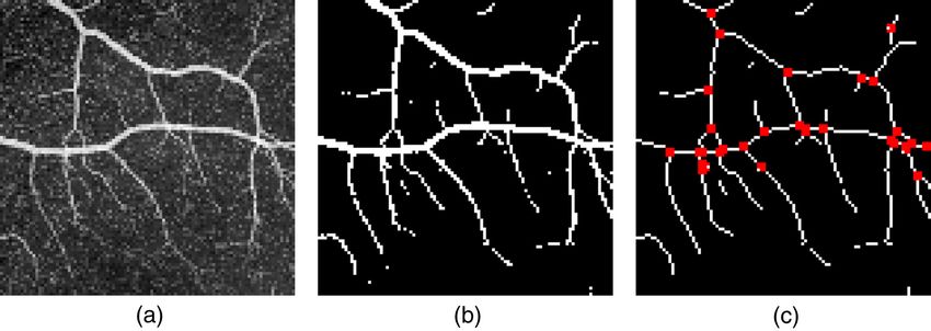
Guimarães et al.: Three-dimensional segmentation and reconstruction of the retinal vasculature. . .

                                                                                                   within the OCT volume, and the 3-D modeling of the vascular
                                                                                                   network from the human retina, dealing with crossovers and
                                                                                                   bifurcations. The workflow of this process can be found
                                                                                                   in Fig. 3.

                                                                                                   3.1     Vessel Caliber Estimation
                                                                                                   The lateral resolution of OCT combined with the optical proper-
                                                                                                   ties of the vessel walls do not allow for their direct observation.
                                                                                                   As such, vessel caliber can only be estimated from the shadow
                                                                                                   cast over the RPE due to light absorption by hemoglobin. Due to
                                                                                                   the aforementioned reasons (Sec. 2.2), the PCF ocular fundus
                Fig. 3 Flowchart for the 3-D segmentation block of Fig. 1. The main                reference image is the natural choice for the vessel caliber esti-
                block inputs are the OCT volume, the segmented layers, the 2-D ocu-                mation. Thus, it is clear that the estimated caliber is below the
                lar fundus reference image, and the binary image (Fig. 2).                         real caliber and that this effect is less significant for larger ves-
                                                                                                   sels closer to the optic disk, and become more important close to
                                                                                                   the fovea as vessels become thinner. In addition, the estimated
                    All four 2-D fundus reference images computed from
                                                                                                   caliber can only be achieved in the xy plane and we assume them
                OCT volumes (MVF, EVF, ELM, and PCF) were used as
                                                                                                   to have a circular cross section.
                features in the classification process. Additional features were
                                                                                                       There is a wealth of literature on methods to compute retinal
                computed from the PCF image. Specifically, intensity-
                based features, local-phase features, and features computed                        vessel width from 2-D ocular fundus images. These were tail-
                with Gaussian-derivative filters, log-Gabor and average filter                     ored for imaging modalities such as CFP and FA.27–29 These
                banks, and bandpass filters were obtained.23 A supervised learn-                   methods rely on the estimation of the cross section with respect
                ing algorithm (support vector machine) was then used to train                      to vessel centerlines and have to deal with the rough definition
                and classify each A-scan of the OCT volume V into vessel or                        of vessel borders due to the regular sampling of the digital im-
                nonvessel A-scans, i.e., to discriminate between A-scans that                      aging modalities.30,31 This effect is much more prominent on
                cross retinal blood vessels and the remaining A-scans.                             OCT rendering these methods inappropriate for this modality.
                Formally, we define the set A ¼ fAi ð:Þ∶∀i ∈ Ug of A-scans                             Log-Gabor wavelets are routinely used for vessel enhance-
                Ai ð:Þ ¼ Vðxi ; yi ; : : : Þ that cross vessels. The set U is defined              ment and detection.32 These are created by combining a radial
                as the indices of A-scans that cross vessels.                                      and an angular component (in the frequency space), then deter-
                    The process proved able to cope with OCTs of both healthy                      mining the scale and the orientation of the filter, respectively. In
                and diseased retinas. It achieved good results for both the mac-                   the time domain, the filter is composed by even (real part) and
                ular and optic nerve head regions. For a set of macular OCT                        odd (imaginary part) kernels.
                scans of healthy subjects and diabetic patients, the algorithm                         To determine the retinal vessels’ caliber, the PCF image is
                achieved 98% accuracy, 99% specificity, and 83% sensitivity.                       filtered with a bank of log-Gabor even kernels, each with a
                For both groups, the algorithm favorably compared to the                           unique orientation-scale pair. This bank covers a wide range
                inter-grader agreement.23                                                          of scales and orientations to fully describe the whole vascular
                                                                                                   network. At each vessel pixel PCFðxi ; yi Þ, with i ∈ U, the
                                                                                                   log-Gabor even kernel whose orientation-scale pair
                3     Three-Dimensional Segmentation and                                           better matches the vessel orientation and caliber generates the
                      Reconstruction                                                               highest response. The scale of the kernel with the maximal
                The core of the work presented in this paper addresses the issues                  response can then be translated into the caliber of the vessel
                of estimating vessels diameters and their depth-wise location                      on that pixel.

                                       Fig. 4 Examples of 2-D vessel binary maps cropped to bewildering regions of crossovers and/or
                                       bifurcations.

                Journal of Biomedical Optics                                               016006-3                                          January 2015   •   Vol. 20(1)

Downloaded From: https://www.spiedigitallibrary.org/journals/Journal-of-Biomedical-Optics on 13 Jun 2022
Terms of Use: https://www.spiedigitallibrary.org/terms-of-use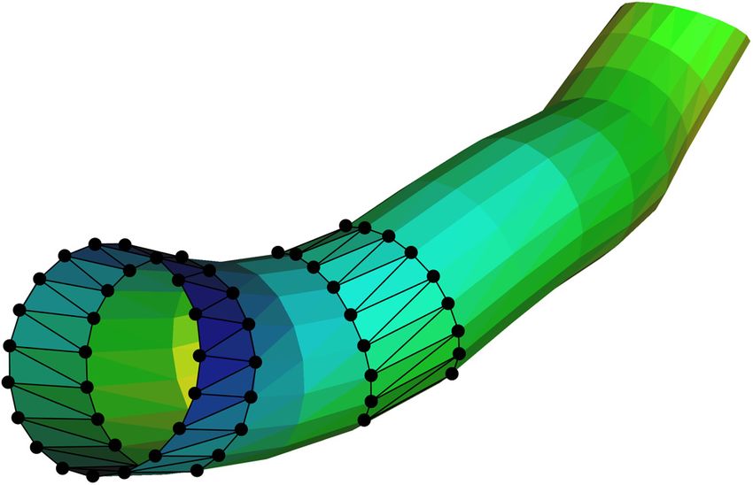
Guimarães et al.: Three-dimensional segmentation and reconstruction of the retinal vasculature. . .

                                       Fig. 5 Detail of a principal component fundus reference image (a) and the respective binary maps of
                                       the 2-D classification U (b) and of the vessel centerlines (with the removed bewildering regions in
                                       red) Uskel (c).

                3.2     Bewildering Regions                                                        these are removed (erased) from the skeleton image. In conse-
                                                                                                   quence, all potential bifurcations and crossovers are adequately
                The bewildering regions are subsets of neighboring vascular net-                   left to be re-linked. This new set of points defines the set
                work A-scans where the path of the vessels is unclear from the                     U skel (Fig. 5).
                2-D segmentation due to bifurcation and/or crossovers (Fig. 4).                        The set E c ⊂ U skel of endpoints on each bewildering region c,
                To determine these regions, several binary morphological oper-                     with E c ∈ fE 1 ; E 2 ; : : : g, will then be used to look for the most
                ations are used. These regions require further processing                          plausible linking configuration of that region (Sec. 3.4).
                (see Sec. 3.4).
                    First, endpoints in the vicinity of one another on the binary
                                                                                                   3.3     Vascular Network Depth-Wise Position
                vascular fundus image are bridged and the binary image (the set
                of vessel points U) is redefined. This updated image is then                       As stated, retinal blood vessels are not directly visible in stan-
                skeletonized and isolated points are removed. Finally, the bewil-                  dard OCT data. Typically, vessels on OCT appear as hyper-
                dering regions are defined as the dilation of branch points and                    reflective regions followed posteriorly by the shadowing of

                                       Fig. 6 Computation examples of the depth coordinate of different blood vessel at a centerline point i. The
                                       two profiles on the top of each plot are the vessel profile Avessel
                                                                                                     i     (blue) and the nonvessel profile Anonvessel
                                                                                                                                              i
                                       (red). The difference between the two (black profile) is shown on the bottom. The difference profile is
                                       filtered at the region of interest (green) and the depth coordinate of the vessel on that point is taken as the
                                       location of the maximum of the filtered difference.

                Journal of Biomedical Optics                                               016006-4                                            January 2015   •   Vol. 20(1)

Downloaded From: https://www.spiedigitallibrary.org/journals/Journal-of-Biomedical-Optics on 13 Jun 2022
Terms of Use: https://www.spiedigitallibrary.org/terms-of-use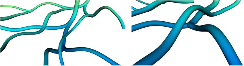
Guimarães et al.: Three-dimensional segmentation and reconstruction of the retinal vasculature. . .

                structures beneath due to light absorption by hemoglobin in per-                   where si is the estimated caliber at the i‘th A-scan,  is the con-
                fused vessels.                                                                     volution operator, and ci is restricted to be in the inter-
                    In the previous section, all A-scans were classified as vessel                 val ½Z1 þ si ∕2; Z2 − si ∕2.
                or nonvessel A-scans. Only A-scans from the centerline of the
                vessel are processed to search for the depth-wise location of the                  3.4     Bifurcations and Crossovers
                vessel, using the following methods.
                                                                                                   Vessel tracking in OCT is quite different from other imaging
                                                                                                   modalities. Due to the low sampling of OCT systems compared
                3.3.1    Principal Component Analysis                                              to imaging modalities as CFP and FA, most vessels are just one
                                                                                                   to two pixels wide and the bewildering regions present many
                PCA is used to enhance similar information between neighbor                        alternatives for the linking process in windows just a few pixels
                vessel A-scans in the principal component. For each vessel                         wide (Fig. 4). Furthermore, since we use the shadow to locate
                centerline A-scan (Askel ¼ fAi ð:Þ∶∀i ∈ U skel g), a circular                      the blood vessels, the intensity of different vessels on the fundus
                region in the xy plane centered at ðxi ; yi Þ with radius r is                     reference images do not differ sufficiently to tell them apart.
                defined. The set of A-scans in each vessel and nonvessel region                        As a preprocessing step before linkage, we screen all the pos-
                is used to compute two new profiles, Avessel and Anonvessel ,                      sible links to find those that are unlikely and to find some links
                respectively, as follows:                                                          that were not established in the 2-D classification that could help
                    Every A-scan within the defined region is interpolated to                      in solving the bewildering region (the so-called growing links).
                account for differences in retinal thickness, from the ILM                         All possible links are then subject to thresholding by length,
                (Z1 ) to the IS/OS (Z2 ). One should bear in mind that the                         angle between linked vessel segments, and angle between
                whole volume was previously flattened by the IS/OS layer26                         each vessel segment and the link itself.
                and, as such, Z2 is now equal for all A-scans.                                         For each bewildering region c, a cost ϕij is assigned to every
                    Each profile in Avessel ¼ fAvessel
                                                i      ð:Þ∶∀i ∈ U skel g is computed               link lij between every two points, ðxi ; yi ; zi Þ and ðxj ; yj ; zj Þ,
                as the principal component of the selected A-scans Aj such that                    such that fi; jg ∈ E c and i < j, as

                                                                                                 ϕij ¼ ðαij þ βij þ γ ij Þðαji þ βji þ γ ji Þ
                Aj ∶½xi − xj ; yi − yj

                                          < r;       ∀fi; jg ∈ V k ;                   (1)                                                                                (4)

                                                                                                   with
                where V k ⊂ U is the set of indices of the A-scans that constitute
                                                                                                        2  xy         yj − yi
                the vessel k and k:k; is the usual Euclidean norm. On the other                    αij ¼ θi − arctan
                hand, each profile in Anonvessel ¼ fAnonvessel ð:Þ∶∀i ∈ U skel g is                     π               xj − xi
                                                         i
                computed as the principal component of the selected A-scans                                    minðsi ; sj Þ
                Aj such that                                                                       βij ¼ 1 −
                                                                                                              maxðsi ; sj Þ
                                                                                                                      0                          1

                Aj ∶½xi − xj ; yi − yj
                                                     ∀j ∈
                                                         = U:                                                                     zj − zi
                                          < r;                                         (2)               2 z           B                       A
                                                                                                                                                    C
                                                                                                    γ ij ¼ θi − arctan@                                                 (5)
                                                                                                          π                 ½xi − xj ; yi − yj

                   At the first iteration, the sets V k ∈ fV 1 ; V 2 ; : : : g are vessel
                segments delimited by bewildering regions. However, after
                defining the actual links between segments, the depth-wise posi-                   with arctan and the difference of angles mapped to the interval
                tion can be recomputed to improve the estimation at the bewil-                     ½−π∕2; π∕2, and θxy and θz are, respectively, the orientations of
                dering regions (Fig. 3).                                                           the vessel in the xy plane and in z.
                   Although the radius r was empirically selected following vis-                      At this point, we shall define all configurations
                ual inspection of the final 3-D segmentation, it is now kept fixed                 Ck ∈ fC1 ; C2 ; : : : g as sets of links lij subject to the following
                for the processing of all the examples.                                            constraints:

                                                                                                       • the set of links contains the link with the least
                3.3.2    Local Difference Profiles                                                         cost (lij ∶ði; jÞ ¼ argmini;j ϕij );
                                                                                                       • all end-points have to be linked, except points that need
                To estimate the z (depth) coordinate of the vessel at each point of
                the centerline, the difference between the vessel ðAvessel Þ and the                       vessel segmentation growing to link between them;
                                                                     i
                nonvessel ðAnonvessel
                              i       Þ profiles is computed for each i ∈ U skel .                     • there is only one link by vessel segmentation growing;
                This operation results in a difference profile with two clear sig-                     • the configuration does not result in intersections or loops
                natures, one due to the presence of the hyper reflectivity and the                         in the same vessel.
                other due to the shadow in vessel A-scans only, as illustrated
                in Fig. 6.                                                                            Generally, the set fC1 ; C2 ; : : : g will enclose all possibilities
                    Although the vessel walls are not seen in the difference pro-                  for crossovers and bifurcations.
                file, one can estimate their position (and, therefore, the vessel                     The cost of the configuration Ck is then computed as
                cener) by taking advantage of its diameter estimated in                                        X
                                                                                                   Φk ¼                     ϕij :                                          (6)
                Sec. 3.1. A moving average filter hðx; dÞ with size d allows
                                                                                                           ði;jÞ∶∀lij ∈Ck
                for the estimation of the center of the vessel by
                                                                                                      From the group of many feasible combinations, i.e., ignoring
                ci ¼ arg max½ðAvessel
                               i      ðzÞ − Anonvessel
                                             i         ðzÞÞ  hðz; si Þ;               (3)        the ones rendering loops within the same vessel, the solution
                            z                                                                      presenting the lowest overall cost is chosen.

                Journal of Biomedical Optics                                               016006-5                                               January 2015   •   Vol. 20(1)

Downloaded From: https://www.spiedigitallibrary.org/journals/Journal-of-Biomedical-Optics on 13 Jun 2022
Terms of Use: https://www.spiedigitallibrary.org/terms-of-use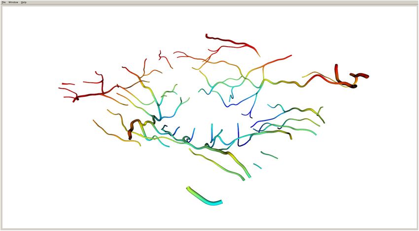
Guimarães et al.: Three-dimensional segmentation and reconstruction of the retinal vasculature. . .

                3.5     Three-Dimensional Reconstruction                                           4       Results
                Vessel centerlines in the xy plane (Sec. 3.2) are combined with                    OCT macular scans of 15 eyes from healthy subjects and eyes
                the estimated vessel centerlines of Sec. 3.4 to render the 3-D                     from patients diagnosed with type 2 diabetes mellitus (early
                skeleton on the vascular network.                                                  treatment diabetic retinopathy study levels 10 to 35) were
                    In this work, we assume vessels to have a local tubular struc-                 used as the test bed for the proposed methodology. All OCT
                ture whose centerlines are defined by the 3-D skeleton and the                     scans were gathered from our institutional database and were
                diameter is estimated from the fundus reference image (xy                          collected by a Cirrus HD-OCT (Carl Zeiss Meditec, Dublin,
                plane). In this way, cylinders and cone-like structures are the                    CA, United States) system. These eyes were also imaged by
                fundamental components from which the 3-D vascular network                         CFP (Zeiss FF 450 system) and/or FA (Topcon TRC 50DX,
                is built.                                                                          Topcon Medical Systems, Inc., Oakland, NJ, United States).
                                                                                                       The results obtained for the 3-D vascular segmentation are
                                                                                                   now presented in three parts: the vessel caliber estimation,
                3.5.1    Vessels Path Interpolation
                                                                                                   the bewildering regions decision, and the reconstruction and
                The combination of vessel diameter and low OCT sampling                            z position of the vessels.
                results in vessels is poorly defined in the fundus reference. In
                addition, at vessel crossovers, the basic assumptions for the                      4.1      Vessel Caliber
                determination of the vessel depth location are no longer verified
                except for the top one. That is, the vessels below the top one do                  The automated vessel caliber estimation was compared with the
                not present the clear signatures (vessel hyper reflectivity and                    assisted estimates made by three graders (G1 , G2 , and G3 ).
                shadow) since they lie on the shadow cast by the vessel                                Five vessel segments per OCT eye scan were randomly
                above. In this way, interpolation is mandatory and is performed                    chosen, each with a minimum of 21 pixels long along the center-
                under the assumption that vessels do not present discontinuities                   line. Graders were instructed to use a software tool. Since the
                or sharp edges, i.e., they are continuous with respect to the first                lateral sampling of OCT is relatively low, the graders would not
                derivative in any of the three dimensions. Under these assump-                     be able to simply mark the vessel boundaries, as is the common
                tions, the vascular network is built based on OCT data (control                    practice for CFP.33 Instead, the tool provided for any given cal-
                points) making use of cubic spline interpolation.                                  iber, a subpixel continuous marking of the boundaries (for that
                                                                                                   particular caliber) of the whole vessel segment against the PCF
                                                                                                   image. Several diameters with increments of 0.2 pixels were
                3.5.2    Delaunay Triangulation
                                                                                                   tested by the graders to choose the diameter that best fits the
                Vessel reconstruction is achieved by Delaunay triangulation. At                    data. The result is a set of several caliber measurements (in pix-
                each vessel centerline location, the tangent to the path, defined                  els) for each randomly chosen vessel segment.
                by the centerline points, is computed and the respective normal                        For the comparison, two metrics were used, the absolute and
                plane determined. The cross section of the vessel is approxi-                      the relative differences as defined, respectively, by
                mated by a set of points in this cross-sectional plane within
                the circumference centered at the vessel centerline and a diam-                    Da ðG; GÞ
                                                                                                          ^ ¼ jG − Gj;
                                                                                                                   ^                                                      (7)
                eter equal to the estimated vessel’s diameter (Fig. 7). Adjacent
                circumferences are later connected using the Delaunay triangu-
                lation in 3-D. The quality of the final reconstruction is directly                 Dr ðG; GÞ
                                                                                                          ^ ¼ jG − Gj∕
                                                                                                                   ^ G;^                                                  (8)
                dependent on the number of triangles, which in turn depends on
                                                                                                                                   ^ is the ground truth, considered
                                                                                                   where G is the data to test and G
                the circumference sampling and the gap between estimated ves-
                sel cross sections.                                                                here as the average of all the graders (Table 1).

                                                                                                   Table 1 Comparison between the automatic caliber estimation (S)
                                                                                                   and each manual grading (G 1 , G 2 , and G 3 ), by the mean and stan-
                                                                                                   dard deviation (SD) values for the absolute difference D a (pixels) and
                                                                                                   the relative difference D r between the result G and G.^

                                                                                                   Metric          G                 ^
                                                                                                                                     G                  Mean            SD

                                                                                                           ^
                                                                                                   D a ðG; GÞ        S      1∕3ðG 1 þ G 2 þ G 3 Þ       0.311          0.208

                                                                                                                   G1          1∕2ðG 2 þ G 3 Þ          0.494          0.240

                                                                                                                   G2          1∕2ðG 1 þ G 3 Þ          0.187          0.153

                                                                                                                   G3          1∕2ðG 1 þ G 2 Þ          0.406          0.231

                                                                                                           ^
                                                                                                   D r ðG; GÞ        S      1∕3ðG 1 þ G 2 þ G 3 Þ       0.213          0.173
                Fig. 7 Illustration of a local reconstruction of a vessel, based on                                G1          1∕2ðG 2 þ G 3 Þ          0.299          0.168
                Delaunay triangulation. Several points over the centerline are chosen
                and equally distant points (with distance equal to the estimated radius                            G2          1∕2ðG 1 þ G 3 Þ          0.122          0.110
                of the vessel in the x y plane) in the respective orthogonal plane to the
                centerline are considered for the 3-D triangulation process of                                     G3          1∕2ðG 1 þ G 2 Þ          0.337          0.266
                reconstruction.

                Journal of Biomedical Optics                                               016006-6                                              January 2015   •   Vol. 20(1)

Downloaded From: https://www.spiedigitallibrary.org/journals/Journal-of-Biomedical-Optics on 13 Jun 2022
Terms of Use: https://www.spiedigitallibrary.org/terms-of-use
Guimarães et al.: Three-dimensional segmentation and reconstruction of the retinal vasculature. . .
0.6 0.6 0.6 0.6
0.5 0.5 0.5 0.5
0.4 0.4 0.4 0.4
0.3 0.3 0.3 0.3
0.2 0.2 0.2 0.2
0.1 0.1 0.1 0.1
0 0 0 0
1 2 3 4 1 2 3 4 1 2 3 4 1 2 3 4
Caliber (pixels) Caliber (pixels) Caliber (pixels) Caliber (pixels)
Fig. 8 Average relative differences for the automatic estimation (S) and manual gradings (G 1 , G 2 , and
G 3 ) displayed by caliber range.
Table 1 shows the average metric results by comparing the depending on the number of possibilities for each region.
automatic estimation (S) to the average grading of all graders This was demonstrated to be a very demanding task for the auto-
and each grader to the average grading of the other two, as a matic process. For very difficult cases or whenever graders
measure of inter-grader agreement. Figure 8 shows the relative decided, they could access either a fluorescein angiography
difference metric for several ranges of diameters for the same or CFP, or both, according to the respective availability in
comparisons. As expected, smaller vessels render a higher vari- our database. In general, the access to these complementary im-
ability as shown by the histograms. Figure 9 shows both the aging modalities proved to be frequently required for this task.
manual and automatic determination of vessel boudaries over
Three metrics were used to assess the accuracy of the automated
the PCF fundus reference image.
system in establishing the correct links between vessel segments
at bewildering regions. These are: the point accuracy (indicates
4.2 Bewildering Regions
the percentage of points in E c correctly grouped), the linking
At bifurcation and crossover locations, the continuity of each accuracy (the percentage of links correctly connected and non-
vessel is hard to detect even for a human grader, naturally links correctly unconnect, i.e., the percentage of true positives
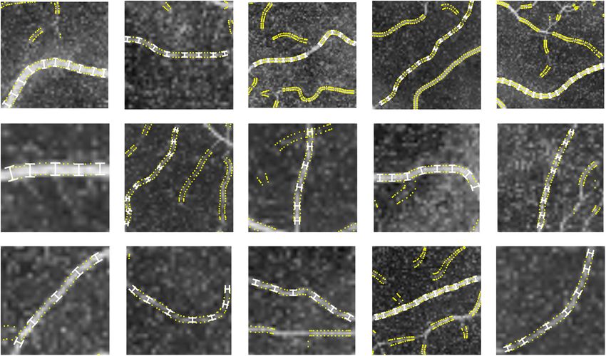
Fig. 9 Representative results for the diameter estimation. The manual gradings are marked with (white)
⊢⊣; and automatic estimation is marked with the (yellow) dotted line.
Journal of Biomedical Optics 016006-7 January 2015 • Vol. 20(1)
Downloaded From: https://www.spiedigitallibrary.org/journals/Journal-of-Biomedical-Optics on 13 Jun 2022
Terms of Use: https://www.spiedigitallibrary.org/terms-of-useGuimarães et al.: Three-dimensional segmentation and reconstruction of the retinal vasculature. . .
# regions point accuracy linking accuracy bewildering accuracy
150
90
90
90
80
80
80
70 70
70
100
60 60
60
50 50
50
%
%
%
40 40
40
50 30
30 30
20 20 20
10 10 10
0 0 0 0
3 4 5 6 7 8 9 1011 3 4 5 6 7 8 9 1011 3 4 5 6 7 8 9 1011 3 4 5 6 7 8 9 1011
# points # points # points # points
Fig. 10 Number of bewildering regions by number of points to link (points in Ec ), on the left, and metric
results for bewildering region solving.
and false negatives) and, the percentage of bewildered regions as the graders found it very difficult to evaluate them. Both grad-
correctly classified. ers evaluated the same A-scans so that inter-grader variability
The results are shown in Figs. 10 and 11. was computed. A software tool was developed to help in this
process. The second grader repeated the process (G5.2 ) to estab-
lish an intra-grader variability. The results are shown in Fig. 12
4.3 Vascular Network Depth-Wise Position and summarized in Table 2.
The low visibility of vessel markers (such as the shadow) ren- The high inter and intra-variability values obtained (0.020
ders the manual detection of blood vessels in OCT B-scans a and 0.011 mm, respectively), clearly show how difficult the
hard task. Two graders (G4 and G5.1 ) were instructed to manual process is.
mark, at 50 randomly selected vessel A-scans, the position As is visible from Fig. 12, the automatic estimation of the
where the shadow of the vessels began. Some restrictions depth-wise position appears mostly at a higher depth than the
were imposed to the random selection to guarantee an unbiased position estimated by the graders, since the grader aims at
evaluation: the same vessel could not be selected twice and not the beginning of the shadow (vessel top wall) and the algorithm
more than five A-scans per exam were possible. Furthermore, aims at the vessel centerline. Hence, this systematic deviation is
very small vessels (less than two pixels in radius) were excluded expected.
Fig. 11 Detail on the reconstruction of the vessels in bewildering regions, with crossovers and
bifurcations.
Journal of Biomedical Optics 016006-8 January 2015 • Vol. 20(1)
Downloaded From: https://www.spiedigitallibrary.org/journals/Journal-of-Biomedical-Optics on 13 Jun 2022
Terms of Use: https://www.spiedigitallibrary.org/terms-of-useGuimarães et al.: Three-dimensional segmentation and reconstruction of the retinal vasculature. . .
0.1
S-G 4
G 5.1-G4
G 5.2-G4
0.05
0
−0.05
−0.1
Fig. 12 Difference (in millimeters) between the first grader (G 4 ) manual marking of the beginning of the
shadow and the automatic segmentation (S) of the centerline, and both markings of the beginning of the
shadow from the second grader (G 5.1 and G 5.2 ).
Table 2 Comparison between the automatic depth-wise position (S) physicians’ expectations, where the vessels rapidly deviate
and each manual grading (G 4 , G 5.1 , and G 5.2 ), by the mean and stan- to form the crossover. Note that the high axial resolution of
dard deviation (SD) values for the absolute difference D a (mm) OCT is crucial to detect crossovers due to this aspect.
^
between the result G and G. Moreover, we illustrate in Fig. 15 the cross section of the vas-
cular reconstruction in several B-scans. These figures illustrate
Metric G ^
G Mean SD that the method leads to a feasible reconstruction of the posi-
tion and shape of the vascular network within the OCT volu-
^
D a ðG; GÞ S G4 0.013 0.009 metric scan.
From Rodrigues et al.,23 the execution time for the 2-D seg-
S G 5.1 0.030 0.026 mentation process (OCT fundus reference computation, features
G4 G 5.1 0.020 0.021 computation, and support vector machines classification), using
a MATLAB® (The MathWorks Inc., Natick, MA) implementa-
G 5.2 G 5.1 0.011 0.012 tion, was 65.2 1.2 s (N ¼ 15). The system hardware used was
an Intel® Core i7-3770 CPU (Intel Corporation, Santa Clara,
California) at 3.4 GHz.
4.4 Reconstruction The additional execution time to achieve the 3-D
reconstruction, also using a MATLAB implementation, was
The proposed reconstruction seems very feasible. Overall, the 122.3 115.1 s (average standard deviation) on an Intel®
reconstructed vessel network is smooth and behaves as Core i7-4770 CPU at 3.4 GHz. For the 3-D reconstruction,
expected (Figs. 13 and 14). In fact, the details of the crossovers the required time greatly depends on the vessel tree complexity.
of vessels, as illustrated in Fig. 11, are also according to The high standard deviation value reflects this behavior.
Fig. 13 3-D reconstruction of the position and shape of the vessels.
Journal of Biomedical Optics 016006-9 January 2015 • Vol. 20(1)
Downloaded From: https://www.spiedigitallibrary.org/journals/Journal-of-Biomedical-Optics on 13 Jun 2022
Terms of Use: https://www.spiedigitallibrary.org/terms-of-useGuimarães et al.: Three-dimensional segmentation and reconstruction of the retinal vasculature. . .
are quite high for the problem at hand, bearing in mind that OCT
lateral resolution is low (in comparison with other modalities).
To the best of our knowledge, this problem is addressed here for
the first time for OCT data.
The different steps of the validation show that the algorithm
performs well. However, Doppler OCT would be a better ground
truth than manual segmentation. Unfortunately, we have no
access to such a system at our institutions. The high inter
and intra-variability values from the manual gradings indicate
how difficult the manual segmentation is.
The first tests on the relevance of the depth component of
the vascular network of the retina have already been con-
ducted.33 In this preliminary study, it is shown that the
Fig. 14 3-D reconstruction of the retinal vascular network embedded most widely used metric of vessel tortuosity does not have
in the OCT volume. a statistically significant linear relation between 2-D and
3-D metrics. Thus, the use of 3-D tortuosity metrics to corre-
late with disease status might have a significant impact on the
5 Discussion and Conclusions correlation values when compared with those obtained using
The method presents a good overall performance. The location 2-D metrics.
of the vascular tree is (as expected) in the upper third of the It is expected that more severe pathologies would render a
retina. The vessel caliber estimation achieves a precision similar more difficult task to overcome. In the future, we hope to extend
to a human grader and the depth position detection is in agree- our tests to these cases. Although one might slightly anticipate
ment with the known anatomy. However, the linking of the ves- worse results, please note that our goal of early diagnosis of
sels in the defined bewildering regions works well when few pathology requires working with eyes within the early stages
connections are involved, but does not seem to contain enough of disease progression (close to normal).
information to achieve higher accuracy when the number of ves- In the present work, we propose and describe a method to
sels to connect is higher. Apart form the presented cost func- segment and visualize the retinal vascular network in 3-D for
tions, many other approaches were tried leading to similar OCT data. Increased sampling and accuracy would improve
but no better results. Although the bewildering accuracy is the algorithm’s performance and would allow for an objective
about 65%, we note that the linking accuracy and point accuracy validation.
Fig. 15 (a) B-scans and cross section of the vascular reconstruction (in white); (b) the respective position
of the B-scan (white line) with the detected vessels (in red) on the fundus reference image.
Journal of Biomedical Optics 016006-10 January 2015 • Vol. 20(1)
Downloaded From: https://www.spiedigitallibrary.org/journals/Journal-of-Biomedical-Optics on 13 Jun 2022
Terms of Use: https://www.spiedigitallibrary.org/terms-of-useGuimarães et al.: Three-dimensional segmentation and reconstruction of the retinal vasculature. . .
Acknowledgments 17. J. Xu et al., “3D OCT retinal vessel segmentation based on boosting
learning,” in IFMBE Proc. World Congress on Medical Physics and
This work was supported by FCT under the research projects Biomedical Engineering, September 7 to 12, 2009, Munich,
(Project Nos. PTDC/SAU-ENB/111139/2009 and PEST-C/ Germany, O. Dössel and W. C. Schlegel, Eds., pp. 179–182,
SAU/UI3282/2013), and by the COMPETE programs Springer, Berlin Heidelberg (2009).
FCOMP-01-0124-FEDER-015712 and FCOMP-01-0124- 18. R. Kafieh et al., “Vessel segmentation in images of optical coherence
FEDER-037299. The authors would like to thank António tomography using shadow information and thickening of retinal nerve
fiber layer,” in Proc. 2013 IEEE Int. Conf. on Acoustics, Speech and
Correia for performing the manual gradings. Signal Processing, pp. 1075–1079, IEEE, Vancouver (2013).
19. M. Pilch et al., “Automated segmentation of retinal blood vessels in
spectral domain optical coherence tomography scans,” Biomed. Opt.
References Express 3, 1478–1491 (2012).
1. G. Liew et al., “Retinal vascular imaging: a new tool in microvascular 20. Z. Hu et al., “Automated segmentation of 3-D spectral OCT retinal
disease research,” Circ. Cardiovasc. Imaging 1(2), 156–161 (2008). blood vessels by neural canal opening false positive suppression,”
2. R. Kawasaki et al., “Retinal microvascular signs and 10-year risk of Lec. Notes Comput. Sci. 13, 33–40 (2010).
cerebral atrophy: the Atherosclerosis Risk in Communities (ARIC) 21. V. Kajić et al., “Automated three-dimensional choroidal vessel segmen-
study,” Stroke 41, 1826–1828 (2010). tation of 3d 1060 nm oct retinal data,” Biomed. Opt. Express 4(1), 134–
3. N. Witt et al., “Abnormalities of retinal microvascular structure and risk 150 (2013).
of mortality from ischemic heart disease and stroke,” Hypertension 47, 22. P. Guimarães et al., “3D retinal vascular network from optical coherence
975–981 (2006). tomography data,” Lec. Notes Comput. Sci., 339–346 (2012).
4. F. N. Doubal et al., “Fractal analysis of retinal vessels suggests that a 23. P. Rodrigues et al., “Two-dimensional segmentation of the retinal vas-
distinct vasculopathy causes lacunar stroke,” Neurology 74, 1102–1107 cular network from optical coherence tomography,” J. Biomed. Opt. 18,
(2010). 126011 (2013).
5. R. Kawasaki et al., “Retinal microvascular signs and risk of stroke: the 24. K. Li et al., “Optimal surface segmentation in volumetric images - a
multi-ethnic study of atherosclerosis (MESA),” Stroke 43, 3245–51 graph-theoretic approach,” IEEE Trans. Pattern Anal. Mach. Intell.
(2012). 28, 119–134 (2006).
6. N. Patton et al., “Retinal vascular image analysis as a potential screening 25. P. A. Dufour et al., “Graph-based multi-surface segmentation of OCT
tool for cerebrovascular disease: a rationale based on homology between data using trained hard and soft constraints,” IEEE Trans. Med. Imaging
cerebral and retinal microvasculatures,” J. Anat. 206, 319–348 (2005). 32, 531–543 (2013).
7. N. Patton et al., “The association between retinal vascular network 26. P. Guimarães et al., “Ocular fundus reference images from optical coher-
geometry and cognitive ability in an elderly population,” Invest. ence tomography,” Comput. Med. Imaging Graph. 38(5), 381–389
Ophthalmol. Vis. Sci. 48, 1995–2000 (2007). (2014).
8. H. Yatsuya et al., “Retinal microvascular abnormalities and risk of lacu- 27. B. Al-Diri, A. Hunter, and D. Steel, “An active contour model for seg-
nar stroke: atherosclerosis risk in communities study,” Stroke 41, 1349– menting and measuring retinal vessels,” IEEE Trans. Med. Imaging 28,
1355 (2010). 1488–1497 (2009).
9. P. Z. Benitez-Aguirre et al., “Retinal vascular geometry predicts incident 28. X. Xu et al., “Vessel boundary delineation on fundus images using
renal dysfunction in young people with type 1 diabetes,” Diabet. Care graph-based approach,” IEEE Trans. Med. Imaging 30, 1184–1191
35, 599–604 (2012). (2011).
10. X. Wang, H. Cao, and J. Zhang, “Analysis of retinal images associated 29. E. Trucco et al., “Novel VAMPIRE algorithms for quantitative analysis
with hypertension and diabetes,” in Proc. 27th Ann. Int. Conf. of the of the retinal vasculature,” in Proc. 2013 ISSNIP Biosignals and
IEEE Engineering in Medicine and Biology Society, Vol. 6, Biorobotics Conference (BRC), pp. 1–4, IEEE, Rio de Janeiro (2013).
pp. 6407–6410, IEEE, Shangai (2005). 30. B. Al-Diri et al., “Manual measurement of retinal bifurcation features.,”
11. M. B. Sasongko et al., “Alterations in retinal microvascular geometry in in Proc. 2010 Ann. Int. Conf. of the IEEE Engineering in Medicine and
young type 1 diabetes,” Diabet. Care 33, 1331–1336 (2010). Biology Society, Buenos Aires, Vol. 2010, pp. 4760–4764 (2010).
12. B. E. Bouma et al., Handbook of Optical Coherence Tomography, 31. B. Al-Diri et al., “Automated analysis of retinal vascular network con-
Marcel Dekker, New York (2002). nectivity,” Comput. Med. Imaging Graph. 34(6), 462–470 (2010).
13. R. Bernardes and J. Cunha-Vaz, Optical Coherence Tomography: A 32. J. V. B. Soares et al., “Retinal vessel segmentation using the 2-D Gabor
Clinical and Technical Update, Springer, Heidelberg (2012). wavelet and supervised classification,” IEEE Trans. Med. Imaging 25,
14. T. Fabritius et al., “Automated retinal shadow compensation of optical 1214–1222 (2006).
coherence tomography images,” J. Biomed. Opt. 14(1), 010503 (2009). 33. P. Serranho et al., “On the relevance of the 3D retinal vascular network
15. W. Drexler and J. G. Fujimoto, Optical Coherence Tomography: from OCT data,” Biometric. Lett. 49, 95–102 (2012).
Technology and Applications, Springer, Heidelberg (2008).
16. M. Niemeijer et al., “Vessel Segmentation in 3D spectral OCT scans of Biographies of the authors are not available.
the retina,” Proc. SPIE 6914, 69141R (2008).
Journal of Biomedical Optics 016006-11 January 2015 • Vol. 20(1)
Downloaded From: https://www.spiedigitallibrary.org/journals/Journal-of-Biomedical-Optics on 13 Jun 2022
Terms of Use: https://www.spiedigitallibrary.org/terms-of-useYou can also read