TIM: modelling pathways to meet Ireland's long-term energy system challenges with the TIMES-Ireland Model (v1.0) - GMD
←
→
Page content transcription
If your browser does not render page correctly, please read the page content below
Model description paper
Geosci. Model Dev., 15, 4991–5019, 2022
https://doi.org/10.5194/gmd-15-4991-2022
© Author(s) 2022. This work is distributed under
the Creative Commons Attribution 4.0 License.

TIM: modelling pathways to meet Ireland’s long-term energy
system challenges with the TIMES-Ireland Model (v1.0)
Olexandr Balyk1,2 , James Glynn1,2,3 , Vahid Aryanpur1,2 , Ankita Gaur1,2 , Jason McGuire1,2 , Andrew Smith1,2 ,
Xiufeng Yue1,2,4 , and Hannah Daly1,2
1 Energy   Policy and Modelling Group, MaREI, the SFI Research Centre for Energy, Climate and Marine,
Environmental Research Institute, University College Cork, Cork, Ireland
2 School of Engineering and Architecture, University College Cork, Cork, Ireland
3 Center on Global Energy Policy, School of International and Public Affairs, Columbia University, New York, NY, USA
4 Institute of Tourism and Environment, School of Economics and Management, Dalian University of Technology,

Dalian City, Liaoning, China

Correspondence: Olexandr Balyk (olexandr.balyk@ucc.ie) and Hannah Daly (h.daly@ucc.ie)

Received: 22 October 2021 – Discussion started: 22 November 2021
Revised: 19 May 2022 – Accepted: 31 May 2022 – Published: 29 June 2022

Abstract. Ireland has significantly increased its climate mit-   pinned by detailed bottom-up sectoral models, cross-model
igation ambition, with a recent government commitment to         harmonisation, and soft-linking with demand and macro
reduce greenhouse gases by an average of 7 % yr−1 in the         models. The paper also outlines a priority list of future model
period to 2030 and a net-zero target for 2050, underpinned       developments to better meet the challenge of deeply decar-
by a series of 5-year carbon budgets. Energy systems opti-       bonising energy supply and demand, taking into account the
misation modelling (ESOM) is a widely used tool to inform        equity, cost-effectiveness, and technical feasibility. To sup-
pathways to address long-term energy challenges. This arti-      port transparency and openness in decision-making, TIM is
cle describes a new ESOM developed to inform Ireland’s en-       available to download under a Creative Commons licence.
ergy system decarbonisation challenge. The TIMES-Ireland
Model (TIM) is an optimisation model of the Irish energy
system, which calculates the cost-optimal fuel and technol-
ogy mix to meet future energy service demands in the trans-      1   Introduction
port, buildings, industry, and agriculture sectors, while re-
specting constraints in greenhouse gas emissions, primary        Ireland faces very significant challenges in meeting greater
energy resources, and feasible deployment rates. TIM is de-      energy needs in the future with a much lower carbon foot-
veloped to take into account Ireland’s unique energy system      print. Ireland has a high per capita carbon footprint rel-
context, including a very high potential for offshore wind       ative to the European Union average (e.g. in 2018, 13.5
energy and the challenge of integrating this on a relatively     vs. 8.6 t CO2 e per capita (European Environmental Agency,
isolated grid, a very ambitious decarbonisation target in the    2022)) and was expected to fail its 2020 decarbonisation ob-
period to 2030, the policy need to inform 5-year carbon bud-     jective as set by the European Union (EU) (DCCAE, 2019).
gets to meet policy targets, and the challenge of decarbon-      Under existing policy measures, overall greenhouse gases
ising heat in the context of low building stock thermal effi-    (GHGs) are projected to be relatively stable in the period to
ciency and high reliance on fossil fuels. To that end, model     2030 and to increase in the period to 2040 (EPA, 2020). In
features of note include future-proofing with flexible tempo-    contrast, the EU’s Effort Sharing Regulation sets forth a leg-
ral and spatial definitions, with a possible hourly time reso-   islated target which increases the Irish decarbonisation ob-
lution, unit commitment and capacity expansion features in       jective to reduce non-emissions traded sector emissions by
the power sector, residential and passenger transport under-     30 % relative to 2005 levels by 2030 (CCAC, 2020). In 2019,
                                                                 the government presented a Climate Action Plan which set

Published by Copernicus Publications on behalf of the European Geosciences Union.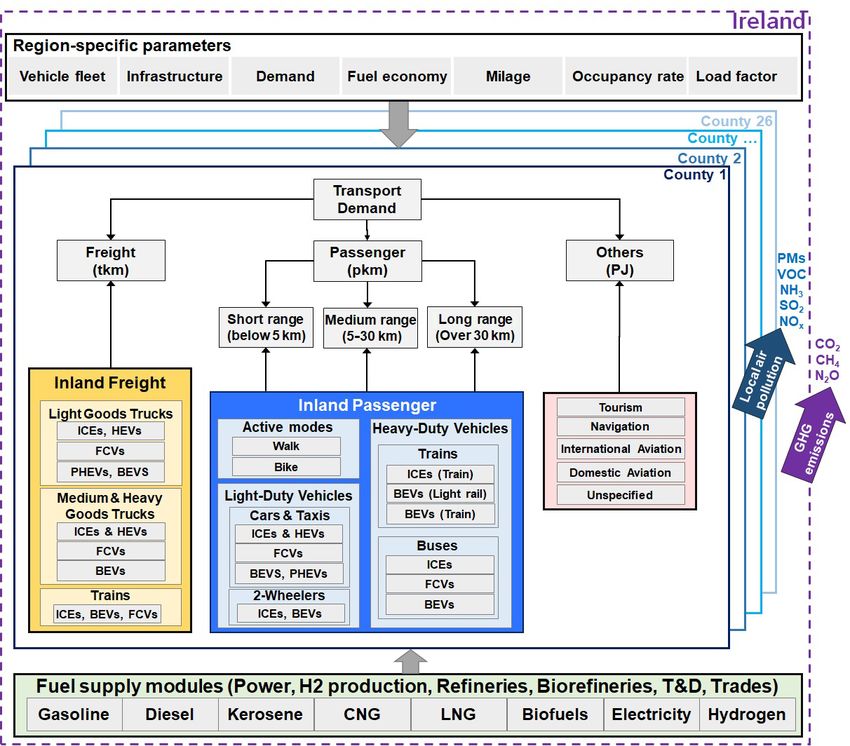
4992                 O. Balyk et al.: Modelling pathways to meet Ireland’s long-term energy system challenges with TIM

forth sector-by-sector measures to meet this increased am-            unforeseen step changes in electricity demand because of,
bition from the EU, which includes increasing the renew-              perhaps, the electrification of transport or of heating.
able electricity share to 70 % by 2030, for electric vehicles            TIM is the successor to the Irish TIMES model (Ó Gal-
to reach full market share later in the decade, and very ambi-        lachóir et al., 2020), which has a long (more than 10 years)
tious targets for retrofitting and electrifying home heating.         history of providing analytical input to Irish energy policy
   However, additional policy measures are needed to reduce           development, including acting as the basis for Ireland’s first
emissions even faster. In 2020, a new government adopted an           low-carbon roadmap in 2015 (Deane et al., 2013) and for de-
even more ambitious decarbonisation target to reduce emis-            veloping energy pathways consistent with the Paris Agree-
sions by 7 % annually in the period to 2030, more than halv-          ment (Glynn et al., 2019), to which Ireland is a signatory.
ing emissions, and planning for a legislated net-zero emis-           TIM is a new model and has been developed to better in-
sions target by 2050 (Department of the Taoiseach, 2020).             form increased national climate mitigation ambition, to take
During the preceding decade, emissions decreased on aver-             into account the changing energy technology landscape, and
age by only about 1 % annually (European Environmental                to take advantage of new advances in energy systems opti-
Agency, 2022).                                                        misation modelling techniques, which are described in the
   Ireland faces a number of challenges in meeting these ob-          remainder of this paper.
jectives. First, a very high share of GHG emissions (34 % in             Internationally, TIMES models are used in a number of
2018 (Duffy et al., 2019)1 ) in Ireland arise in the agricultural     countries to understand and plan for long-term energy tran-
sector, which is a large and export-led part of the economy,          sitions, including in Denmark (Balyk et al., 2019), Ukraine
dominated by beef and dairy production, with an emissions             (Petrović et al., 2021), and the United Kingdom (Fais et al.,
profile which is considered more difficult to abate than en-          2016; Daly et al., 2015).
ergy sectors. Slower mitigation in this sector will require en-          Other energy system models in Ireland which are used to
ergy to decarbonise faster. Second, transport and heating are         inform long-term pathways include the LEAP-Ireland model
heavily dependent on fossil fuels (with shares of 94 % and            (Mac Uidhir et al., 2020; Rogan et al., 2014), based on a sim-
96 % of consumption, respectively; SEAI, 2019), while dis-            ulation approach, which is being co-developed with TIM to
persed settlement patterns and an inefficient building stock          take advantage of data harmonisation and complement pol-
make improving efficiencies challenging. Third, while Ire-            icy insights. Furthermore, the Economic and Social Research
land has already been successful in generating 42 % of its            Institute (ESRI) develops the I3E model, a top-down com-
electricity from renewables in 2020, 86 % of which came               putable general equilibrium (CGE) model (see Sect. 2.6).
from wind energy (SEAI, 2021), the relatively isolated nature         The 2019 Climate Action Plan was informed by McKinsey’s
of the electricity grid and lack of alternative low-carbon elec-      marginal abatement cost curve (MACC) (DCCAE, 2019).
tricity sources will make it very challenging to integrate high          TIM is a significant step forward in the national energy
shares of renewable electricity. The TIMES-Ireland Model              systems modelling capacity. A number of features better en-
(TIM) has been built to offer mitigation solutions taking             able this model to capture long-term energy systems transi-
these challenges into account (Balyk et al., 2021).                   tions, enabling it to better inform very ambitious decarboni-
   Energy system models have long been used to inform de-             sation targets. These features are described in detail through-
carbonisation policies both in Ireland and other countries. In-       out the paper and are summarised in Sect. 4.
tegrated and dynamic energy systems models have a num-                   The rest of the paper is structured as follows: Sect. 2 gives
ber of advantages over single-sector or static approaches.            a general description of the model, including a plain English
Current energy systems are the result of complex country-             description of the model (Sect. 2.1), an outline of the TIMES
dependent, multi-sector developments. The complex dynam-              methodology and model generator (Sect. 2.2), an overview
ics (incorporating technologies, fuel prices, infrastructures,        of the system (Sect. 2.3), the temporal and regional charac-
and capacity constraints) of the entire energy system can be          teristics (Sect. 2.4), underlying demand drivers (Sect. 2.5),
analysed through this modelling approach to better inform             and the model development approach (Sect. 2.6). Section 3
policy choices. A key strength is to approach energy as a sys-        describes the model sectors (supply, power, transport, res-
tem rather than as a set of discrete non-interactive elements.        idential, industry, services, and agriculture). Section 4 dis-
This has the advantage of providing insights into the most            cusses model strengths, weaknesses, and priority areas for
important substitution options that are linked to the system          future development. Finally, Appendix A includes additional
as a whole, which cannot be understood when analysing a               technoeconomic assumptions for future technologies.
single technology, commodity, or sector. A single focus on
the electricity sector, for example, risks excluding possible

   1 These emissions are mainly non-CO emissions, CH and
                                      2             4
N2 O, arising from enteric fermentation, fertiliser application and
soil management, and do not include emissions from land use, while
grasslands are a net carbon source.

Geosci. Model Dev., 15, 4991–5019, 2022                                               https://doi.org/10.5194/gmd-15-4991-2022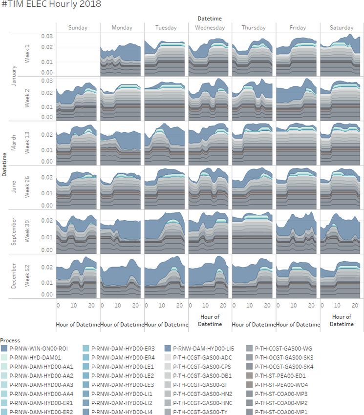
O. Balyk et al.: Modelling pathways to meet Ireland’s long-term energy system challenges with TIM                            4993

2     Model description                                              – Reference energy system (RES), which is the process-
                                                                       flow architecture of economic sectors and energy flows
2.1    Plain English description                                       (commodity) between processes (technology), which
                                                                       consume and produce energy, energy service demands,
The TIMES-Ireland Model produces energy system path-                   and/or other commodities such as environmental emis-
ways for energy supply and demand in Ireland consistent                sions (including greenhouse gases) and other materials.
with either a carbon budget or a decarbonisation target. It            The base year energy flows are calibrated to national
calculates the lowest cost configuration of energy fuels and           energy balances.
technologies which meet future energy demands, while re-
specting technical, environmental, economic, social, and pol-        – Energy service demands are the physical services re-
icy constraints. Key inputs and constraints include primary            quired by the economy and society for mobility, heat,
energy resource availability and costs, the technical and cost         communications, food, etc., which drive energy de-
evolution of new mitigation options, and maximum feasible              mand.
uptake rates of new technologies. Alternatively, TIM can be          – Energy supply curves are the quantities of primary en-
used to assess the implications of certain policies, namely            ergy resources (e.g. wind power) or imported commodi-
regulatory or technology target setting (for example, biofuels         ties (e.g. oil, gas, and bioenergy) available at specific
blending obligation or the sales/stock share target for electric       costs points for differing quality and quantity of energy
vehicles).                                                             commodities.

2.2    TIMES model generator                                         – Technoeconomic parameters of existing and potential
                                                                       future energy technologies are economic parameters in-
TIMES (The Integrated MARKAL-EFOM System) is                           cluding current and projected future investment and
a bottom-up optimisation model generator for energy–                   fixed/variable costs and efficiencies of technologies for
environment systems analysis at various levels of spatial,             energy supply (e.g. solar PV panels, transmission and
temporal, and sectoral resolutions (Loulou et al., 2016a, b).          distribution infrastructure, biorefineries, and hydrogen
The TIMES code, written in GAMS and available under                    production) and energy demand (e.g. electric vehicles,
an open-source licence (IEA-ETSAP, 2020), is developed                 natural gas boilers, and carbon capture and storage).
and maintained by the Energy Technology Systems Analy-                 Technological parameters include the transformation ef-
sis Programme (ETSAP; https://iea-etsap.org/, last access:             ficiency, availability factor, capacity factor, and emis-
18 May 2022), a Technology Collaboration Programme                     sions factor.
(TCP) of the International Energy Agency (IEA), established
in 1976. TIMES models can have single or several regions             – User constraints, which can be any combination of lin-
and are typically rich in technology detail, used for medium-          ear constraints (including fixed, maximum, or mini-
to long-term energy system analysis and planning at a re-              mum bounds on growth, investment, or shares) on tech-
gional, national, or global scale.                                     nologies or fuels. These are typically used to simulate
   TIMES is a linear optimisation, technoeconomic, partial             real-world technology constraints or to simulate pol-
equilibrium model generator which assumes perfectly com-               icy scenarios. A typical user constraint for decarbonisa-
petitive markets and perfect foresight. Model variants enable          tion analysis is limiting total annual or cumulative CO2
myopic foresight, general equilibrium, stochastic program-             emissions to model energy system pathways that meet a
ming, and a variety of multi-objective function options. The           national decarbonisation target.
standard objective function maximises the net total surplus           TIMES outputs the optimal investment and operation level
(the sum of producers’ and consumers’ surpluses) which, in         of all energy technologies which meet future energy service
a perfect market with perfect foresight, equates to maximis-       demands at least cost, while respecting user constraints. The
ing the net present value (NPV) of the whole energy system,        model also produces corresponding energy flows, emissions,
maximising societal welfare. Profits, taxes, and subsidies are     and marginal prices of energy and emissions flows.
internal transfers, i.e. occurring within the economy, that do
not change the NPV (albeit that taxes and subsidies can be         2.3   Model architecture
included to influence the optimisation). It calculates the en-
ergy system specification which minimises the discounted to-       Figure 1 shows a simplified RES in TIM. It describes the
tal energy system costs over the model time horizon, which         structure and energy flows including two major parts, i.e.
is the sum of investments, fixed and variable costs, fuel im-      the supply side and demand side. The former comprises en-
port costs, and export revenues for all the modelled processes     ergy resources, fuel production and conversion technologies
less the potential salvage values of investments for which the     (e.g. biorefineries, hydrogen production, and different power
whole lifetime goes beyond the model time horizon.                 plants), transmission, and distribution infrastructure (e.g. gas
   The user inputs the following to the model generator:           pipelines and power grid). The latter covers end-use sectors

https://doi.org/10.5194/gmd-15-4991-2022                                             Geosci. Model Dev., 15, 4991–5019, 2022
4994 O. Balyk et al.: Modelling pathways to meet Ireland’s long-term energy system challenges with TIM
Figure 1. Simplified representation of reference energy system in TIM.
(e.g. transport and residential) and the corresponding energy lic Spending Code (O’Callaghan and Prior, 2018). This rate
service demands (i.e. passenger, freight, and hot water). En- is consistent with García-Gusano et al. (2016), who recom-
ergy resources incorporate both domestic fossil-based fuels mend using a maximum value of 4 %–5 % for the social dis-
and renewable resource potential. These fuels are processed count rate in ESOMs.
and then distributed across the country. End-use technolo- Technology-specific discount rates (also known as hur-
gies consume energy commodities to meet energy service dle rates) are typically used in ESOMs to capture invest-
demands. GHG emissions from fossil fuels combustion and ment decision-making from the individual user or industry
process-related emissions in industry are tracked with the perspective to capture market imperfections, limited finance,
fuel supply module, electricity generation technologies, and and behavioural heuristics, which limit the uptake of novel
sectoral consumption levels. or capital-intensive investments, even when they are cost-
The model’s base year is 2018, and all energy flows, emis- optimal. These parameters are not used in the core version
sions, and energy technology stocks are calibrated to the of TIM, given its use for modelling long-term energy system
2018 energy balance (SEAI, 2019). pathways from a societal perspective. However, variants of
The discount rate, the degree to which future values are the model can be developed to simulate real-world impacts
discounted to the present, is a key parameter in the TIMES of policies and behaviour, which can include hurdle rates
objective function. A social discount rate reflects how soci- (Aryanpur et al., 2022).
ety views present costs and benefits against future ones and
is lower than a financial discount rate, which is how firms 2.4 Time and geography
make investment decisions. In appraising potential projects
or investments, the government applies a social discount rate. TIM has been developed with a deep knowledge of the ge-
Broadly speaking, in an energy systems optimisation mod- ography of the Irish energy system. A special spatiotemporal
elling (ESOM) scenario with a carbon budget constraint, a approach was taken in the RES base year specification and
higher discount rate would promote later decarbonisation and scenario file data structures to allow flexible regional defini-
fewer capital-intensive technology choices. In this model, a tions and temporal resolution in TIM. The model can run in
discount rate of 4 % is applied, which is based on a social multiple modes with multiple configurations of regional and
rate of time preference methodology, as set forth in the Pub- temporal resolution, ranging from a single region national
model at a single annual time slice, all the way to 26 counties
Geosci. Model Dev., 15, 4991–5019, 2022 https://doi.org/10.5194/gmd-15-4991-2022O. Balyk et al.: Modelling pathways to meet Ireland’s long-term energy system challenges with TIM 4995
at hourly resolution where supply–demand data are available Table 1. Population.
at that spatiotemporal granularity (electricity, gas, and trans-
port). Year Population (millions)
High temporal granularity is needed to appropriately 2018 4.85
model energy futures with high variable renewable energy 2020 4.98
systems integration, especially in scenarios with high levels 2030 5.40
of electrification of end-use demands. At the same time, high 2040 5.82
temporal granularity can be computationally expensive and 2050 6.19
can significantly increase the time required for model devel-
opment and testing. In TIM, we address this issue by con-
straining all time slice model input data to a single file gen- – Historical gross value added (GVA) for the required
erated with a specific temporal resolution. A time slice tool NACE (statistical classification of economic activities
is used to aggregate raw time series data and create a file in in the European community) categories in the services
the required format (Balyk, 2022). and industry sectors is obtained from the EUROSTAT
High spatial granularity is required to give greater pol- database. Projections for GVA are from the Ireland En-
icy clarity on optimal investment needs based on region- and vironment, Energy, and Economy (I3E) model (Yakut
county-specific characteristics to enable the counteraction of and de Bruin, 2020).
socioeconomic challenges such as energy poverty and in-
frastructure development within an optimisation framework – Gross domestic product (GDP), both historical and fu-
(Aryanpur et al., 2021). We address this in TIM by creating ture projections, is obtained from OECD (2018).
model input data structures that allow specifying data and
formulating constraints on both national and county levels. – Income and historical values of total incomes are taken
Internal file switches, and user shell options, could then be from CSO (2021). Assumptions about income growth in
used to apply TIM on either of the levels. the future are from the National Transport Model (AE-
We have decided to focus on this data-driven spatiotempo- COM, 2019).
ral model set-up to future-proof TIM and enable future Irish
energy policy research needs as data availability improves – Modified gross national income (GNI∗ ) is derived from
during TIM’s lifespan. the Central Statistics Office (CSO) labour force scenario
combined with a forecast for output per person (CSO,
2.5 Demands: drivers and projections 2018).
Energy service demands in end-use sectors are driven by 2.5.3 Energy service demands
growth in the population and in the economy. The model is
set up to allow for alternative scenarios for these drivers, re- Table 2 lists the energy service demands in TIM along with
sulting in different energy service demand projections in the their corresponding drivers and values for 2018 and 2050.
end-use sectors, e.g. as applied in Gaur et al. (2022a, b). This Specifics of the methodologies for projecting each energy
section describes baseline driver projections with a detailed service demand are detailed in later sections, for transport
description of energy service demand projections included in (Sect. 3.3), residential (Sect. 3.4), industry (Sect. 3.5), and
the respective sector sections. services (Sect. 3.6).
2.5.1 Population 2.6 Development approach
Historical population estimates and future projections are ob- TIM has been developed with the goal of achieving best-
tained from CSO (2020d). We use the M2F1 scenario since it practice standards in software development and open mod-
represents a medium growth in population and is in line with elling convention. A Git-centred model development process
population projections used in other national sources (Yakut has been an integral part of the model development approach
and de Bruin, 2020). to enable version control and model management. Along
with improvements in management, quality assurance, and
2.5.2 Economic growth transparency this brings, it also allows developers and re-
searchers from different projects to branch research versions
Economic growth projections are mostly taken from national of the model to explore innovations and new developments,
sources to ensure internal consistency. Gross value added while keeping a secure and stable main version of the model
(GVA) and income projections are modelling outcomes from for policy application. At the same time, individual projects
Bergin et al. (2017) and used by national sources. The fol- and researchers can input their improvements and develop-
lowing historical and projected data are used: ments to the core model to enable continuous improvements.
https://doi.org/10.5194/gmd-15-4991-2022 Geosci. Model Dev., 15, 4991–5019, 20224996 O. Balyk et al.: Modelling pathways to meet Ireland’s long-term energy system challenges with TIM
Table 2. Energy service demands in TIM.
Energy service demand Driver/projection source Value Unit
2018 2050
Non-energy mining GVA per capita, population 2.07 0.13 PJ
Food and beverages GVA per capita, population 22.25 34.00 PJ
Textiles and textile products GVA per capita, population 1.20 4.97 PJ
Wood and wood products GVA per capita, Population 6.69 7.65 PJ
Pulp, paper, publishing, and printing GVA per capita, population 0.67 2.31 PJ
Chemicals and man-made fibres GVA per capita, population 10.60 13.11 PJ
Rubber and plastic products GVA per capita, population 1.14 0.89 PJ
Other non-metallic mineral products Modified investment, GNI∗ 17.77 24.82 PJ
Basic metals and fabricated metal products GVA per capita, population 19.54 21.73 PJ
Machinery and equipment n.e.c. GVA per capita, population 1.29 1.69 PJ
Electrical and optical equipment demand GVA per capita, population 4.27 16.37 PJ
Transport equipment manufacture GVA per capita, population 0.17 0.04 PJ
Other manufacturing GVA per capita, population 4.25 6.12 PJ
Construction GVA per capita, population 4.02 5.90 PJ
Transport demand: short-range passenger travels Income, population 14.56 21.07 Bpkm
Transport demand: medium-range passenger travels Income, population 31.28 45.29 Bpkm
Transport demand: long-range passenger travels Income, population 27.13 38.97 Bpkm
Transport demand: goods vehicles for freight Growth rate (AECOM, 2019) 11.54 25.14 Btkm
Transport demand: tourism fuel None, linear decrease assumed 7.72 0.00 PJ
Transport demand: navigation fuel GDP 3.51 10.04 PJ
Transport demand: unspecified fuel None, linear decrease assumed 21.78 0.00 PJ
Transport demand: aviation domestic None, assumed constant 0.23 0.23 PJ
Transport demand: aviation international International aviation passengers 45.94 62.63 PJ
Residential apartment demand Population 206.80 628.93 000’
Residential attached demand Population 766.35 1056.50 000’
Residential detached demand Population 724.43 889.76 000’
Services – commercial services GNI∗ 28.90 47.39 Mm2
Services – public services GNI∗ 58.15 95.35 Mm2
Services – commercial services – data centres EirGrid (2017) 5.63 40.30 PJ
Services – public services – public lighting Government of Ireland (2018) 0.48 0.58 Mlamps
The abbreviations used in the table are as follows: Bpkm – billion passenger kilometres, Btkm – billion tonne kilometres, and Mlamps – million lamps.
TIM is freely available, which is a prerequisite for trans- els, give more robust analytical insights for policy, and to
parency, repeatable research, model maintenance, and en- share and exchange expertise between the modelling teams.
hancement and verification of results (Pfenninger et al., This also facilitates multimodel approaches to energy sys-
2018). tems modelling, which can make use of harmonised hybrid
Web-based dashboards (https://tim-review1.netlify.app/ frameworks coupling simulation and optimisation simultane-
results/, last access: 18 May 2022) have been extensively ously (Rogan et al., 2014).
used in the model development process, both for internal TIM has also been developed to enable soft-linking
model diagnostics and for external engagement and review. with the Ireland Environment, Energy, and Economy (I3E)
The first TIM scenario results archive has also been pub- macroeconomic model developed at the Economic and So-
lished on Zenodo (Daly et al., 2021). cial Research Institute (ESRI; Yakut and de Bruin, 2020).
TIM has been co-developed with the LEAP-Ireland model I3E is a single-country, multi-sector (NACE) inter-temporal
(Mac Uidhir et al., 2020), which is a bottom-up simulation computable general equilibrium (CGE) model focusing on
model of the Irish energy system which simulates the im- environmental and energy accounts in Ireland. While COre
pact of different policy measures and targets on overall GHG Structural MOdel for Ireland (COSMO) focuses on the in-
emissions in Ireland, with a particularly granular represen- fluence of monetary and fiscal policy on economic activ-
tation of transport and residential heat demand. Underlying ity in Ireland, I3E supplements the macroeconomic outlook
data for the relevant sectors are shared between TIM and from COSMO with environmental and energy disaggrega-
LEAP using a data repository and a shared coding conven- tion. I3E retrieves economic growth rates and population es-
tion dictionary to improve the consistency between the mod- timates from COSMO. TIM derives macroeconomic drivers
Geosci. Model Dev., 15, 4991–5019, 2022 https://doi.org/10.5194/gmd-15-4991-2022O. Balyk et al.: Modelling pathways to meet Ireland’s long-term energy system challenges with TIM 4997
coupled to the output variables of I3E, enabling scenario 3.1.3 Emissions tracking
variants based on alternative monetary, fiscal, and macroe-
conomic futures, as well as rapid energy system outlook up- The environmental emissions from each primary energy
dates aligned with the update cycle of the macroeconomic commodity are tracked on the basis of energy- and process-
outlooks from the ESRI. based emissions via combustion and activity-based emis-
sions intensity factors, calibrated on a sector-by-sector ba-
sis. Within the supply sector, methane, nitrogen dioxide, sul-
3 Sectors fur dioxide, carbon dioxide, nitrogen oxide, and particulate
matter can be tracked in the sector’s emissions accounting
3.1 Supply balance. In the current version of TIM, biomass is assumed
to be carbon neutral. However, future versions of the model
3.1.1 Overview
may include different assumptions on emissions linked to use
The supply sector (SUP) in TIM represents the primary and of biomass.
secondary energy commodities and the processes by which
3.1.4 Import/export
those same commodities are imported, exported, domesti-
cally produced through mining or capture of renewable en- Primary and secondary energy commodities, both fossil en-
ergy potentials, and transformed or refined for end-use con- ergy and bioenergy, are imported from international markets
sumption within the energy system both in the base year at international prices. There are no constraints on the im-
(2018) and into the future. The supply sector declares the fu- port quantity of oil and coal, as it is assumed that interna-
ture available routes for commodity trade for the import and tional markets can supply domestic demand and that there
export of energy commodities in terms of the quantity of en- is sufficient on island storage aligned with International En-
ergy and in terms of import capacity through ports, pipelines, ergy Agency – Organisation for Economic Co-operation and
and interconnectors at any given time in the model horizon. Development (IEA-OECD) energy security protocols. Im-
ported gas via pipeline and liquefied petroleum gas (LPG)
3.1.2 Energy balance and commodity declarations
are modelled on an annual basis. Bidirectional electricity in-
Building the supply sector begins with declaring the energy terconnectors to the UK are also represented. Greenlink and
commodities as per the SEAI (2019) energy balance, as re- Celtic interconnectors are assumed operational from 2023
ported to the International Energy Agency. Care is taken and 2026, respectively.
to ensure best-practice coding conventions are followed for
3.1.5 Fuel prices
each commodity – coal, oil, gas, first- and second-generation
bioenergy (biogas, bioliquids, and solid biomass), liquid and Fuel prices for each imported energy commodity are sourced
gaseous hydrogen, wind, solar, geothermal, wave, tidal, mu- from IEA (2019, 2020). Secondary commodity import prices
nicipal wastes, agriculture wastes, and industrial food waste. are index linked to the primary commodities by a price ratio
Active transport time for walking and cycling is also de- on the basis of the current ratio between primary and sec-
clared. All base year commodities are declared in the supply ondary commodity prices. For example, imported gasoline
sector to maintain clear, tidy, and transparent data structures is assumed to be 1.65 times the price of crude oil per unit
within TIM. energy.
The model development team co-created a convention dic-
tionary workbook within the main repository that utilises au- 3.1.6 Domestic energy resources
tomated three-letter coding conventions for technology, com-
modity, and file name creation. This designed and followed Domestic fossil fuel reserves for the production of natural
code convention enables the clean creation of process sets, gas from both the Corrib and Kinsale gas fields and the pro-
commodity sets, results sets, and data automation routines for duction of peat are calibrated with two-step supply curves.
preprocessing and postprocessing data inputs, data outputs, These supply curves are constrained in terms of cumulative
and results. Ultimately, this makes the model architecture energy reserves, annual production costs, and annual produc-
more transparent and easy to develop, enabling new users tion output in energy terms to account for typical production
into the community of developers and peer review. More- profiles from each field.
over, setting out a predefined and intuitive commodity nam- Renewable energy potentials (hydro, wind, solar, waste,
ing convention and a dictionary that is shared across TIM and ocean, geothermal, and ambient heat) are declared in the sup-
LEAP-Ireland has multiple benefits for the multimodel cou- ply sector but are calibrated and constrained in their relevant
pling, diagnostics, and results reporting that are discussed. sectors, such as power generation and transport.
https://doi.org/10.5194/gmd-15-4991-2022 Geosci. Model Dev., 15, 4991–5019, 20224998 O. Balyk et al.: Modelling pathways to meet Ireland’s long-term energy system challenges with TIM
3.1.7 Bioenergy potentials 3.1.11 Hydrogen
Bioenergy potentials are calibrated to SEAI (2015), both in Hydrogen production is modelled, distinguishing future in-
terms of sustainable import volume availability and domestic vestments in centralised and decentralised electrolysis op-
production potential. Domestic bioenergy potentials such as tions. Delivery options are disaggregated and costed at high
sawmill residues, post-consumer recycled wood, municipal pressure for both transmission and distribution pipelines and
waste, tallow, recovered vegetable oil, straw, animal waste, a road tanker option for distribution. Hydrogen storage is also
and industrial food wastes are modelled with three-step sup- modelled within TIM at the finest time slice level, allowing
ply curves in terms of price and quantities available. Crop- hourly production and consumption of hydrogen to be rep-
based bioenergy feedstocks are modelled within the agricul- resented. This is particularly useful for modelling electricity
ture sector. Domestic bioenergy supply potentials and costs grid balancing with unit commitment, dispatch, and capacity
are sensitive to scenarios narrative and, as such, are modelled expansion, while capturing variable renewable energy system
within scenario files to account for uncertainty. dynamics.
3.1.8 Refineries 3.2 Electricity
Ireland has only one oil refinery, i.e. Whitegate in County
3.2.1 Overview
Cork. It is calibrated to import crude oil at international
prices and converts crude oil to refined products limited by
Ireland has a high share of variable renewable electricity for
the upper bounds of output shares, such that the output has
a relatively isolated grid, with 32.5 % of electricity genera-
flexible upper shares of 22.9 % gasoline, 8.1 % kerosene,
tion in 2019 coming from onshore wind energy. Achieving
40.9 % diesel, and 34.4 % heavy fuel oil. The refinery is con-
the 2020 electricity from renewable energy sources (RES-E)
strained to stay at current capacity, has a lifespan of 50 years,
target has encouraged strong growth in onshore wind, while
and the production costs are differentiated by production
increasing the non-synchronous penetration of renewables to
(flow) costs for each output fuel.
70 % by 2030, including offshore wind development, is a key
3.1.9 Electricity interconnectors policy objective over the next decade as Ireland moves to-
wards a net-zero carbon electricity system.
Existing electricity interconnectors to the UK are calibrated
such that exports are priced 30 % lower than imports. The 3.2.2 Existing dispatchable grid
2018 export and import quantities of electricity are calibrated
as per historical data. The future activity is constrained us- The existing 61 generation unit fleet is calibrated to the
ing upper bounds, given that TIM does not model the UK base year of 2018 from the Commission for Energy Regula-
electricity market other than through a predefined price sig- tion (CRU) I-SEM validated PLEXOS model (Geffert et al.,
nal. This constrain can be relaxed but is used to explore do- 2018). Each existing generation unit can be explicitly mod-
mestic needs for system flexibility, security, system services, elled with a possibility to use unit commitment within TIM.
and storage. Neither reinforcement of existing interconnec- This model configuration includes the generation unit capac-
tors nor investment in new interconnectors is currently in- ity, the fuel type of each generation unit, the start-up costs
cluded in the model. (from cold, warm, and hot), the efficiency curve of the gen-
eration unit to include startup and shutdown phases, startup
3.1.10 Biorefineries and shutdown times (cold, warm, and hot), the ramp rates,
minimum load, efficiency at minimum load, minimum up-
Future biorefinery technologies are defined in the supply time and minimum downtime, the unit lifespan, the unit an-
sector future technology (SubRES) database. The follow- nual availability, and the start year of the unit (Geffert et al.,
ing technologies are defined: (1) ethanol production from 2018). The near-term generation unit pipeline is calibrated
wheat, woody biomass, and grass, (2) biodiesel production to EirGrid and SONI (2019, 2020) to account for early clo-
from oilseed rape (OSR), woody biomass, industrial food sures of units before their economic lifespan, which largely
waste, recovered vegetable oil (RVO), and tallow, (3) wood takes into account coal- and peat-based plants during the next
pellets production from biomass, and (4) biogas production decade. We have not forced a new capacity of future planned
from grass, woody biomass, municipal waste, industrial food power plants from EirGrid and SONI (2020) in TIM, which
waste, and animal wastes. All biorefining technologies are includes recent battery storage installations. These recent and
defined in terms of the start year, efficiency, investment costs, planned units can be forced via a scenario file.
availability factor, and the operation and maintenance costs. Existing 302 onshore and 1 offshore wind farms within the
Irish Wind Energy Association database currently operate as
a single aggregated generation pool governed by historical
hourly availability factors for wind generation from 2018.
Geosci. Model Dev., 15, 4991–5019, 2022 https://doi.org/10.5194/gmd-15-4991-2022O. Balyk et al.: Modelling pathways to meet Ireland’s long-term energy system challenges with TIM 4999
Figure 2. TIM hourly unit commitment modelling capabilities example for 2018.
3.2.3 Future electricity system Renewable energy potentials are based on a number of
sources. Total energy resource availability of solar and
New generation capacity investment costs, fixed and variable wind are from Pfenninger and Staffell (2016) and Staffell
operation, and maintenance costs and technical efficiencies and Pfenninger (2016), respectively, with availability factors
are derived from Carlsson et al. (2014). The future unit com- from Ruiz et al. (2019). Ocean and tidal energy potentials are
mitment dispatch operational constraints and cycling costs from O’Rourke et al. (2010), and the wave energy power ma-
are generalised for each technology type based on the fuel trix (for a comprehensive discussion, see, e.g., https://www.
and vintage (Kumar et al., 2012).
https://doi.org/10.5194/gmd-15-4991-2022 Geosci. Model Dev., 15, 4991–5019, 20225000 O. Balyk et al.: Modelling pathways to meet Ireland’s long-term energy system challenges with TIM
Table 3. Onshore wind connection cost.
Capacity (GW) Connection cost (EUR per kW)
0–8.1 25
8.1–16.8 39
16.8–22.6 69
22.6–26.6 153
26.6–30.6 358
sciencedirect.com/topics/engineering/matrix-power, last ac-
cess: 18 May 2022) is derived from Nambiar et al. (2016).
Hourly availability factors for ocean energy technologies are
derived from the marine institute and Office of Public Works’
data buoy services.
Future onshore wind energy potential has been assessed
at high spatial resolution using geographic information sys-
tem (GIS) techniques. Wind farm expansion is constrained
by both technology costs and a supply curve for grid con-
nections, based on a GIS analysis of existing houses, special
areas of heritage and conservation, existing grid lines by volt-
age specification, wind energy potential, existing substation
locations, and the costs per kilometre of the standard Elec-
tricity Supply Board (ESB) grid line specifications to con-
nect wind resource potential to the existing grid. The wind
energy potential is defined as a cost curve aggregated from
1938 suitable land parcels from a GIS analysis (Fig. 3). Due
to the fact that increasing both technical details and the tem- Figure 3. Wind energy potential locations.
poral resolution causes exponential increase in model size,
the spatial resolution is simplified and is represented in a
four-step cost curve (Table 3). This can be disaggregated on
a spatial resolution down to each individual parcel of land or moval (CDR) technologies, and negative emission technolo-
on a county-by-county basis. Future wind energy can gener- gies (NETS) are currently seen within the literature as being
ate at the same hourly capacity factor that occurred in 2018 critical future technologies to capture the last marginal resid-
but with capacity expansion. ual emissions to bring the energy system to net-zero CO2 or
Losses from electricity transmission and distribution are even net-negative CO2 by mid-century. With this in mind,
assumed to be 7 %, with no grid expansion costs currently TIM has carbon capture and storage (CCS) technology op-
represented in the model. The maximum share of variable tions available from 2030, including retrofit options on exist-
renewable energy, including wind, solar, and wave energy is ing coal, peat, and gas power plants. Bioenergy carbon cap-
constrained at 75 % by 2030, and 100 % is allowed by 2050. ture and storage (BECCS) is available in TIM from 2030 and
The model technology database includes short-term stor- provides net-negative CO2 capture and allows negative emis-
age battery technologies, medium-term pumped hydro stor- sions electricity generation. Direct air carbon capture and
age, and long-term hydrogen storage. All these storage tech- storage (DACCS) is also defined as a backstop technology,
nology options are typically deployed in hourly unit com- i.e. it has a static unit cost of EUR 2000 per ton of CO2 and
mitment capacity expansion scenarios and provide ancillary an unlimited capacity. This caps the marginal abatement cost
services and balancing in 100 % variable renewable energy of the model at a price that does not exclude any of the plau-
source (VRES) scenarios. sible mitigation measures.
3.2.4 Carbon capture and storage, carbon dioxide
3.2.5 User constraints
removal, and negative emissions technologies
It is well documented in the literature that residual emis- User constraints applied to the power sector in TIM largely
sions are likely to remain in the future (net-)zero carbon en- pertain to the calibration of the near-term shutdown of coal
ergy system from hard-to-decarbonise sectors (Rogelj et al., and peat power plants before their economic lifetime ends as
2018). Carbon capture and storage (CCS), carbon dioxide re- a result of policy decisions.
Geosci. Model Dev., 15, 4991–5019, 2022 https://doi.org/10.5194/gmd-15-4991-2022O. Balyk et al.: Modelling pathways to meet Ireland’s long-term energy system challenges with TIM 5001
3.3 Transport 3.3.2 Future transport demand projections
3.3.1 Overview Passenger kilometres: private cars
The transport sector comprehensively describes the end-use Future passenger car transport demand is projected based on
transport technologies and freight and mobility demands on a future population growth and a growing rate of car owner-
regional basis. This sector is divided into 26 counties across ship, which is in turn determined by income growth. Car
Ireland. To represent region-specific transport characteristics, ownership usually follows an S-shaped function which has
some main parameters (vehicle fleet, transport infrastructure, three periods, i.e. slow growth during low income levels,
fuel consumption, mileage, occupancy rate, and load factor) rapid increase as income levels rise quickly, and finally a
are differentiated on a county level. Transport demand is split saturation period. The Gompertz statistical model has been
into the following three main categories: passenger, freight, found to fit the historical relationship between car ownership
and others. The passenger and freight demands are expressed and income levels best, although other functions have also
as activity demands, and others are defined as a final en- been used in previous studies (Lian et al., 2018). The basic
ergy demand (PJ). These final energy demands further split Gompertz function is shown in Eq. (1).
into aviation (international and domestic), navigation, fuel
−γ x
tourism, and unspecified, aligned with the energy balance y = α · e−β·e , (1)
(SEAI, 2019). Fuel tourism refers to cross-border consumers,
and a portion of demand is used by unspecified modes. where y is the car per adult, α is saturation level of car own-
The passenger transport demands are expressed in billion ership, x is an economic indicator (income per adult in this
passenger kilometres (Bpkm). As shown in Table 4, the to- case), and β, γ are parameters that are estimated using his-
tal passenger demand is divided into three classes of dis- torical data obtained from the CSO.
tance range, including short range (less than 5 km), medium Projection of future car ownership levels is based on
range (5–30 km), and long range (more than 30 km; NTA, change in income levels. The saturation level of car owner-
2018). A total of four transport modes satisfy travel demands, ship is assumed at 875 per 1000 adults (AECOM, 2019). Car
namely public services (bus, train, and taxi), private cars, ownership (cars per adult) is projected to rise from 0.56 in
powered two-wheelers (PTW), and active modes (walk and 2018 to 0.69 in 2050, an increase of 23 %. Passenger kilo-
bike). Non-motorised transport is only used for short-range metres are then derived using car ownership as a proxy and
trips, PTW are used for short- and medium-range travel, ur- assuming an occupancy level of 1.492 and kilometres per car
ban buses and school buses are used for short- and medium- to remain constant at about 17 300 yr−1 . Total passenger kilo-
range travel, intercity buses and heavy trains are used for metres from private cars in 2050 is projected to increase by
long-range trips, and light rail can only be used for the 42 % from the 2018 level, with a compound annual growth
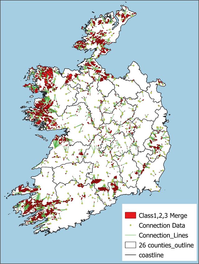
short- and medium-range trips in Dublin county. As shown rate (CAGR) of 1.1 %. The growth rate of passenger kilome-
in Fig. 4, the demand for each mode can be met with a differ- tres from private cars was 1.35 % between 2008 and 2018.
ent set of technologies, based on cost-optimisation and user
constraints. The base year is calibrated based on the actual Passenger kilometres: other modes of transport
number of vehicles and the corresponding vehicle activities.
Mode-specific relation between distance ranges is assumed Other modes of transport represent a much smaller share of
constant throughout the modelling horizon (can be derived mobility demand compared to private cars. Passenger kilo-
from Table 4). Total future passenger demand is obtained as metres of large public service vehicles (PSVs) are projected
a sum of mode-specific demand projections, as described in using population as a driver in a log function and assuming an
Sect. 3.3.2. Table 6 shows vehicle characteristics on a na- average occupancy of 27.5. Large PSV passenger kilometres
tional basis. are expected to increase by 24.2 % in 2050, as compared to
The inland freight demand is expressed in billion tonne those in 2018, with a CAGR of 0.7 %. Passenger kilometres
kilometres (Btkm). It comprises two main modes, i.e. goods of other modes (luas, train, small PSVs, and motorcycles)
trucks and trains. The definition of light and heavy goods and active modes (walking and cycling) are projected using
vehicles varies in different studies. In this model, they are population as a driver. The passenger kilometres are expected
disaggregated by the following three unladen weight bands to increase by 60 % with a CAGR of 1.5 %.
(CSO, 2020g, h, i): light-duty trucks (below 5 t), medium-
International aviation fuel demand
duty trucks (5–10 t), and heavy-duty trucks (over 10 t). Ta-
ble 5 shows freight demand in the base year in million tonne International aviation fuel demand is projected using number
kilometres (Mtkm); the modal shares are assumed constant of passengers as a driver. The number of aviation passengers
throughout the modelling horizon. is projected using damped Holt–Winters function based on
historical time series data obtained from CSO (Dantas et al.,
2017; Grubb and Mason, 2001). The number of passengers
https://doi.org/10.5194/gmd-15-4991-2022 Geosci. Model Dev., 15, 4991–5019, 20225002 O. Balyk et al.: Modelling pathways to meet Ireland’s long-term energy system challenges with TIM
Table 4. Total passenger demand and share of transport modes for each class of distance range (CSO, 2017, 2020c, e, f, g, h).
Modes Vehicles Short range Medium range Long range
(below 5 km) (5–30 km) (over 30 km)
Public Bus 8.3 % 13.5 % 16.1 %
Light train 0.8 % 0.7 % n/a
Heavy train n/a n/a 8.4 %
Taxi 1.7 % 2.2 % 1.3 %
Private Car 51.5 % 83.3 % 74.2 %
Powered two-wheelers 0.1 % 0.3 % n/a
Active Bike 5.4 % n/a n/a
Walk 32.2 % n/a n/a
Total passenger demand in 2018 (Bpkm) 14.6 31.3 27.1
n/a: not applicable
Table 5. Freight demand in 2018 (CSO, 2020g, h, i).
Classification Unladen weight (t) Demand (Mtkm) Share (%)
Light-duty trucks 0–5 292 2.5
Medium-duty trucks 5–10 1140 9.8
Heavy-duty trucks over 10 10 106 86.9
Train – 89 0.8
Total freight demand 11 627 100
in 2050 is expected to increase by 45.5 % compared to 2018. (BioCNG), hydrogen, and dual-fuel engines (running
The historical fuel demand for aviation and number of avia- either on gasoline or CNG/BioCNG, each one taking
tion passengers are then used as input for a linear regression 50 % of the distance travelled) and compression ignition
model to project the future demand for aviation fuel. The fuel engines powered by diesel and biodiesel.
demand in 2050 increases by 37 % relative to 2018 with a
CAGR of 1 %. 2. Hybrid electric vehicles (HEVs) are equipped with an
ICE, which provides the main power, and a small elec-
Other transport fuel demand tric motor to support the ICE and to recuperate the brak-
ing energy.
Demand for freight is projected using growth rates from AE-
3. Plug-in hybrid electric vehicles (PHEVs) have a simi-
COM (2019). The growth in tonne kilometres of freight is
lar power train to HEVs. Their batteries can be charged
expected to increase by 1.18 times in 2050 from 2018 levels
from the grid for driving tens of kilometres solely on
with a CAGR of 2.5 %. Navigation fuel demand is projected
electrical power. We assume the maximum distance
using GDP as the explanatory variable. Fuel demand for nav-
driven on electric mode is 50 % in the base year, and
igation in 2050 is expected to increase 2.85 times compared
it can increase to 80 % over time.
to 2018 with a CAGR of 3.3 %. Fuel tourism is assumed to
remain constant at 11 PJ. 4. Battery electric vehicles (BEVs) solely rely on batteries,
which provide the total motive power of the vehicle. The
3.3.3 Future technology options batteries charge from the grid.
Common vehicle technologies and future options that are 5. Fuel cell vehicles (FCVs) are electrochemical devices
likely to become available for future investment shape the that produce electricity through a reaction between hy-
technology database for the transportation sector in TIM. drogen and oxygen. The electricity drives a vehicle’s
They are categorised into five major groups as follows electric motor. Conventional fuel tanks are replaced
(Aryanpur and Shafiei, 2015): with pressurised hydrogen storage tanks in FCVs.
1. Internal combustion engines (ICEs) consist of spark Table A7 shows the technoeconomic characteristics of fu-
ignition engines fuelled by gasoline, bioethanol, ture passenger transport vehicles (Mulholland et al., 2017;
compressed natural gas (CNG), compressed biogas Helgeson and Peter, 2020). Maintenance costs are assumed
Geosci. Model Dev., 15, 4991–5019, 2022 https://doi.org/10.5194/gmd-15-4991-2022O. Balyk et al.: Modelling pathways to meet Ireland’s long-term energy system challenges with TIM 5003
Figure 4. Transport structure in TIM.
to remain constant. Vehicle purchase price parity between improve the retirement profile both for existing and new ve-
BEVs and ICEs is expected in the period 2025–2030. hicles, TIM is equipped with realistic representation of the
All these technologies compete to meet the mobility de- survival profile of car technologies. The survival rates are
mand over the planning horizon. The model structure allows from the Irish CarSTOCK model (Daly and Ó Gallachóir,
competition among stock replacement and fuel substitution 2011; Mulholland et al., 2018).
within a mode. Modal shift may be simulated within each
travel distance band by defining scenario-specific shares for 3.3.4 User constraints
the different modes (e.g., see Table 4).
Different fuels are supplied to the transport sector via four A set of constraints limits fuel and modal shares in transport
separated modules, including supply, power, biorefineries, sector as follows:
and hydrogen modules. In other words, these connections in- – Maximum biodiesel share in passenger and freight
tegrate the transport sector with the entire energy system. transport demand is 4.1 % in the base year.
TIMES models usually use a simplified constant lifetime
– Maximum bioethanol share in passenger and freight
for different vehicles, and thus, the vehicles are retired at the
transport demand is 3.2 % in the base year.
end of that lifetime. However, a detailed analysis of technol-
ogy retirement profiles in Ireland shows that this simplified – Maximum growth rate in new vehicle sales for ad-
representation is far from reality (Mulholland et al., 2018). vanced power trains (HEVs, PHEVs, BEVs, and FCVs)
An actual profile shows a low decay in the beginning years is 16 % yr−1 , which is enforced once the sales of a ve-
and a long tail in the distribution over the longer term. To hicle type reaches 15 % of the total vehicle sales in the
base year.
https://doi.org/10.5194/gmd-15-4991-2022 Geosci. Model Dev., 15, 4991–5019, 20225004 O. Balyk et al.: Modelling pathways to meet Ireland’s long-term energy system challenges with TIM
Table 6. Existing vehicles and the corresponding characteristics in the base year (CSO, 2020j, k, l; Irish Rail, 2018; TII, 2016).
Vehicles Power train Stock Utilisation factor Occupancy rate Fuel consumption
(1000 units) (1000 km yr−1 ) (pass. per vehicle) (MJ per vkm)
Motorcycle Gasoline ICE 39.85 2.73 1.10 1.70
Cars Gasoline ICE 946.86 12.82 1.49 2.47
Diesel ICE 1129.40 20.62 1.49 2.30
Dual-fuel ICE 0.07 13.44 1.49 2.89
ICE E85 8.53 13.44 1.49 2.41
Gasoline HEV 29.80 12.82 1.49 2.05
Diesel HEV 0.77 20.62 1.49 2.03
Gasoline PHEV 2.76 12.82 1.49 1.56
Diesel PHEV 0.03 20.62 1.49 1.58
BEV 4.53 13.44 1.49 0.85
Taxi Gasoline ICE 2.50 35.61 1.49 2.63
Diesel ICE 17.46 39.93 1.49 2.39
Gasoline HEV 1.35 41.21 1.49 2.03
Bus Diesel ICE 10.70 36.10 27.25 10.16
Train Light train (electric) 0.07 55.69 78.0 24.81
Heavy train (electric) 0.05 158.48 78.0 24.81
Heavy train (diesel) 0.014 73.88 120.0 76.92
vkm: vehicle kilometres.
Table 7. Number of dwellings by type (in thousands). Figure 5 shows the RES diagram for the residential sec-
tor. Energy service demands are disaggregated between
Year Apartment Attached Detached archetype and non-archetype demands. Archetype demands
2018 207 766 724
are energy service demands which depend on the house type,
2030 355 918 833 namely the dwelling type and building energy rating (BER)
2040 493 1003 878 rating.
2050 629 1057 890 The base year residential energy demand by fuel is cali-
brated to the SEAI (2019) energy balance.
Archetype energy service demands are particularly depen-
– The blend limit for biofuels is 10 %–12 % for the regu- dent on the type of building. The four energy service de-
lar ICEs without any modifications (i.e. 10 % bioethanol mands which are modelled based on archetype are space
and 12 % biodiesel, with 90 % and 88 % gasoline and heating, water heating, pump and fans, and lighting. The res-
diesel, respectively). idential building stock by type is explicitly modelled in TIM
in three archetypes, i.e. detached, attached, and apartments.
– Total biofuel supply for the transport sector is allowed The archetype energy service demand data are sourced
to double each decade, reflecting the rate of growth be- from SEAI (2020)’s BER database, which contains the raw
tween 2010 and 2020 (NORA, 2021). data of 906 048 BER surveys. The BER database was fil-
tered before use to remove outliers and any nonsensical val-
3.4 Residential sector ues. The filters were based upon Dineen et al. (2015), Uid-
hir et al. (2020a), and group discussions within the Irish
3.4.1 Energy service demands and projections Building Stock Observatory (https://www.marei.ie/project/
irish-building-stock-observatory/, last access: 18 May 2022),
The residential stock projections up to 2040 are taken from reducing the total records to 815 246.
Bergin and García-Rodríguez (2020) housing demand es- The filtered BER database is projected onto the total
timates, which utilise economic growth projections from dwelling stock, using data from CSO (2020a, b) to calculate
Bergin et al. (2017). The stock is expected to increase by the total number BER ratings per archetype in the dwelling
40 % from 2018 levels with a CAGR of 2 %. This results in stock, as shown in Table 8.
an average of 27 600 new houses per annum between 2021– BER assumes all buildings are heated to between 18 ◦ C
2040. Beyond 2040, the population is used as a driver to for non-living areas (e.g. bedroom and bathroom) to 21 ◦ C
project housing stock. The total housing stock obtained in for living areas (e.g. sitting room and kitchen). This assump-
2050 is 2.57 million dwellings, which implies 8 % increase tion is based on ISO 13790 calculations. To reflect the actual
from 2040.
Geosci. Model Dev., 15, 4991–5019, 2022 https://doi.org/10.5194/gmd-15-4991-2022You can also read