April 2020, Revised June 2021
←
→
Page content transcription
If your browser does not render page correctly, please read the page content below
NBER WORKING PAPER SERIES

              TECHNOLOGICAL INNOVATION AND LABOR INCOME RISK

                                        Leonid Kogan
                                     Dimitris Papanikolaou
                                    Lawrence D. W. Schmidt
                                           Jae Song

                                      Working Paper 26964
                              http://www.nber.org/papers/w26964

                     NATIONAL BUREAU OF ECONOMIC RESEARCH
                              1050 Massachusetts Avenue
                                Cambridge, MA 02138
                            April 2020, Revised June 2021

The research reported herein was performed pursuant to a grant from the U.S. Social Security
Administration (SSA) funded as part of the Retirement and Disability Research Consortium. The
authors also gratefully acknowledge financial support from the Becker-Friedman Institute for
Research in Economics and the MIT Sloan School of Management. We thank Ufuk Akcigit,
Nicholas Bloom, Carter Braxton, Stephane Bonhomme, Jack Favilukis, Carola Frydman, David
Hémous, Gregor Jarosch, Thibaut Lamadon, Ilse Lindenlaub, Elena Manresa, Adrien Matray,
Derek Neal, Serdar Ozkan, Monika Piazzesi, Luigi Pistaferri, Nikolai Roussanov, Martin
Schneider, Toni Whited, and seminar participants in the Social Security Administration, Bank of
Portugal, CEAR/GSU, Carnegie Mellon, Duke University, Duke/UNC Asset Pricing Conference,
University of Chicago, UNC, the LAEF/Advances in Macro Finance workshop, Minnesota Asset
Pricing Conference, Massachusetts Institute of Technology, University of Michigan,
Northwestern, Stanford, University of Pennsylvania, SITE, and Yale for helpful comments and
discussions. We are particularly grateful to Pat Jonas, Kelly Salzmann, and Gerald Ray at the
Social Security Administration for their feedback during our SSA seminar presentation, help, and
support. Further, we thank Josh Rauh, Irina Stefanescu, Jan Bena and Elena Simintzi for sharing
their data and Fatih Guvenen and Serdar Ozkan for sharing their replication code. Brandon
Dixon, Brice Green, Luxi Han, Alejandro Hoyos Suarez, Kyle Kost, Andrei Nagornyi, Bryan
Seegmiller, Jinpu Yang, and Jiaheng Yu provided outstanding research assistance. The views
expressed herein are those of the authors and not necessarily those of the Social Security
Administration. The views expressed herein are those of the authors and not necessarily
those of the Social Security Administration or the National Bureau of Economic Research.

NBER working papers are circulated for discussion and comment purposes. They have not
been peer-reviewed or been subject to the review by the NBER Board of Directors that
accompanies official NBER publications.

© 2020 by Leonid Kogan, Dimitris Papanikolaou, Lawrence D. W. Schmidt, and Jae Song.
All rights reserved. Short sections of text, not to exceed two paragraphs, may be quoted
without explicit permission provided that full credit, including © notice, is given to the source.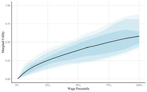
Technological Innovation and Labor Income Risk
Leonid Kogan, Dimitris Papanikolaou, Lawrence D. W. Schmidt, and Jae Song
NBER Working Paper No. 26964
April 2020, Revised June 2021
JEL No. E24,G10,G12

                                             ABSTRACT

Using administrative data from the United States, we document novel stylized facts regarding technological
innovation and the riskiness of labor income. Higher rates of industry innovation are associated with
significant increases in labor earnings for top workers. Decomposing this result, we find that own firm
innovation is associated with a modest increase in the mean, but also variance, of worker earnings
growth. Innovation by competing firms is related to lower, and more negatively skewed, future earnings.
We construct a structural model featuring creative destruction and displacement of human capital that
replicates these patterns. In the model, higher rates of innovation by competing firms increases the
likelihood that both the worker and the incumbent producer are displaced. By contrast, a higher rate
of innovation by the worker's own firm increases profits, but is a mixed blessing for workers, as it
increases odds that the skilled worker is no longer a good match to the new technology. Estimating
the parameters of the model using indirect inference, we find significant welfare losses and hedging
demand against innovation shocks. Consistent with our model, we find that these left tail effects are
more pronounced for process improvements, novel innovations, and are concentrated in movers rather
than continuing workers.

Leonid Kogan                                        Lawrence D. W. Schmidt
MIT Sloan School of Management                      Sloan School of Management
100 Main Street, E62-636                            Massachusetts Institute of Technology
Cambridge, MA 02142                                 100 Main Street
and NBER                                            Cambridge, MA
lkogan@mit.edu                                      ldws@mit.edu

Dimitris Papanikolaou                               Jae Song
Kellogg School of Management                        Social Security Administration
Northwestern University                             Office of Disability Adjudication
2211 Campus Drive, Office 4319                      and Review
Evanston, IL 60208                                  5107 Leesburg Pike, Suite 1400
and NBER                                            Falls Church, VA 22041
d-papanikolaou@kellogg.northwestern.edu             jae.song@ssa.gov
For most households, human capital is the largest component of total wealth. Unlike financial wealth,

human capital is illiquid, poorly diversified, and shocks to its value are largely uninsurable. Thus, un-

derstanding what makes human capital risky is important. Our paper focuses on the role of innovation:

models of creative destruction generate sharp predictions regarding the rate of technological innovation

and redistribution of profits across firms. To the extent that part of a worker’s skill set is specific to a

particular technology vintage or firm or firms share profits with workers, increased rates of innovation

will also affect worker earnings. We explore these ideas in detail and show that there is a strong link

between the rate of technological innovation and risk in worker earnings—particularly for workers at the

top of the earnings distribution, who often have specialized skills and compensation tied to firm profits.

  We begin by presenting a set of new stylized facts using millions of administrative worker earnings

records from the Social Security Administration (SSA) and the firm-level measure of the value of

innovation developed in Kogan, Papanikolaou, Seru, and Stoffman (2017).1 We first examine industry-

level outcomes. We show there is a strong correlation between the rate of technological progress in a

given industry and the variation of future firm profits and worker earnings growth. This correlation is

significantly stronger for workers at the top of the earnings distribution. The rest of the paper focuses

on understanding the drivers of this correlation, and, to that end, for the remainder of the paper we

focus on worker-level outcomes.

  Empirically, we find that the above relation between innovation and human capital risk is driven by

a combination of between- and within-firm effects. We next examine separately the role of innovation

that originates in the workers’ own firm versus other competing firms in the same industry. We find

that increases in the rate of a firm’s own innovations are associated with increased future earnings

growth for its workers. By contrast, an increased rate of innovation by competing firms is associated

with significantly lower future worker earnings. The magnitude of these effects is sizable; the own-firm

effects are consistent with most extant estimates of profit sharing elasticities. However, keeping

constant the associated change in expected firm profits from new innovations, workers’ earnings growth

is more sensitive to innovation by competing firms relative to own firm innovation. Thus, differences in

firm outcomes partly drive workers earnings risk, and workers bear more of that risk on the downside.
   1
    Kogan et al. (2017) propose a measure of the economic importance of each innovation that combines patent data
with the stock market response to news about these patents. An advantage of this measure is that it allows us to connect
each new invention or production method to its originating firm, and therefore isolate innovation by the worker’s own
firm from innovation by its competitors. Kogan et al. (2017) show that their measure is strongly related to changes
in ex-post profitability across firms and document evidence consistent with creative destruction.

                                                           1
These average effects are informative regarding the link between differences in the rate of innovation

across firms and earnings risk. However, they offer an incomplete characterization of effects on income

risk: average effects mask considerable heterogeneity in worker outcomes, even for workers whose

firms innovate at similar rates. Thus, we next use quantile regressions to characterize how the entire

distribution of worker earnings growth rates shifts following innovation by the firm, or its competitors.

We uncover a significant relation between the rate of innovation and the higher moments of the

distribution of earnings growth. Subsequent to innovation by their own firm, the distribution of

earnings growth for the firm’s own workers becomes more positively skewed: the increase in average

earnings we documented above is concentrated among a small subset of workers. Conversely, innovation

by competitors is associated with more negatively skewed earnings growth for the firm’s workers: most

workers experience small declines in income, while a minority experiences a significant drop in labor

earnings. Importantly, these effects are significantly larger in magnitude for the highest paid workers

(top 5% in the distribution of prior earnings within the firm). In addition to larger magnitudes, these

top workers also experience a substantial fattening of the left tail of earnings growth when their own

firm innovates. For these workers, an increase in innovation of their own firm is a mixed blessing, since

it represents a positive shock to both the mean and the variance of their future earnings growth.

  In brief, we uncover an economically significant relation between the rate of technological innovation

and the earnings risk of top workers. This relation is striking given that the existing literature has largely

emphasized the complementarity between technology and high-skill workers (Goldin and Katz, 1998).

To help interpret our facts, we develop a model of innovation and earnings risk. Our model focuses on

high-income (i.e. skilled) workers and has the following key ingredients. Firms compete in the product

market; similar to quality-ladder models, only the most efficient firm finds it profitable to produce in a

given product line. Firm profits (markups) depend on the distance between the leading producer (the

incumbent) and the next most efficient firm (the potential entrant). High rates of innovation by the

entrant result in lower profits by the incumbent firm and potentially the loss of the market for that

product line. Firms hire skilled workers to manage these product lines and these managers’ earnings

are exposed to profits to mitigate a moral hazard friction; hence, there is pass-through of firm profits

to the earnings of top workers. If the firm loses its technology lead in a product line, the incumbent

manager is displaced. Innovation by the worker’s own firm leads to higher profits, but the compatibility

of these innovations with the skills of the incumbent worker is uncertain. That is, the productivity

                                                      2
of the incumbent worker in utilizing the new vintage has a stochastic component and may increase or
decrease; in some cases, the firm may find it profitable to replace the incumbent worker with a new hire.
In sum, the model generates a link between innovation, firm profits, and worker earnings risk. In
the model, innovation by competing firms increases the likelihood that both worker and incumbent
producer are displaced. Thus, it is associated with lower future firm profits and a more negatively
skewed distribution for earnings growth. By contrast, higher rates of own firm innovation lead to
higher average profits but are a mixed blessing for (top) workers, since they increase the likelihood
the manager is no longer a good match to the firm’s technology. Hence, the model generates a higher
mean, but also an increase in the variance of earnings growth of top workers in response to innovation
by their own firm. Exposures are also asymmetric: managers capture only a fraction of the gains from
own firm innovation but fully share in losses from competitor innovation.
We calibrate the model to match our stylized facts above using indirect inference. The model can
quantitatively replicate the key relation between technological progress and earnings risk that we
uncover. In addition, the calibrated model allows us to quantify the impact of innovation on worker
utility. We find that innovation is associated with significant welfare losses for top workers, even in
the presence of progressive taxation and ability to self-insure by accumulating assets. In the model,
the average worker would need to receive a proportional subsidy of 1.5% in her lifetime consumption
to offset the utility loss resulting from a one-standard-deviation (one time, but persistent) increase
in industry innovation. Our estimates thus imply a substantially higher welfare cost of innovation
for (top) workers than the welfare cost of business cycles due to job displacement (Krebs, 2007).
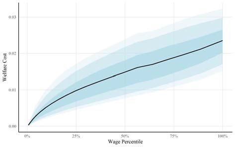
In addition, we use the model to compute the willingness of workers to invest in assets that (partially)
hedge their earnings risk. We find significant demand for insuring changes in the rates of innovation
in the worker’s own industry, as measured by fluctuations in their marginal utility. Specifically, a one
standard deviation increase in industry innovation leads to a 0.38 log point increase (on average) in
the marginal utility of skilled workers. To a first approximation, this estimate implies that workers
would be willing to invest in an asset whose return is maximally correlated with a shock to industry
innovation as long as its Sharpe ratio (market price of risk) was higher than -0.38. That said, there
is dispersion across model workers in the magnitude of these welfare costs and their willingness to
hedge. Similar to the data, higher-income workers in the model face higher risk exposures and are
therefore willing to pay more for insurance.
3Our model has testable predictions that we examine in our data. First, the model generates an
increased left tail of earnings growth through a higher likelihood of job loss. An advantage of our data
is that they allow us to track workers across firms and therefore to examine the extent to which this in-
crease in the risk of earnings declines is related to separations. We therefore explore how the magnitude
of the increase in the left tail varies between stayers (continuing workers) and movers (workers who leave
the firm). In both the model and the data, an increase in the rate of innovation by either the firm or its
competitors is associated with a significantly higher increase in the left tail among movers than stayers.
Further, and consistent with displacement of human capital, incumbent workers are more likely to expe-
rience persistent unemployment spells. As before, these effects are larger in magnitude for top workers.
Second, our model has specific predictions about what types of innovations are more likely to lead
to higher worker earnings risk. In particular, we expect the effects of own firm innovation to be
driven by process (as opposed to product) improvements, and by innovations that are significantly
different from what the firm has done in the past. We measure the former using the process/product
characterization of patents of Bena and Simintzi (2019). We measure novelty using the methodology of
Kelly, Papanikolaou, Seru, and Taddy (2020), who quantify textual similarity across patent documents.
A patent is novel if the description of the innovation is sufficiently distinct from the firm’s prior
innovations. Consistent with our model, we find that the increase in the left tail of (top) worker
earnings is driven by process improvements. By contrast, non-process (product) improvements are
primarily associated with an increase in average earnings rather than an increase in higher moments.
Further, the magnitudes are significantly stronger for innovations that are novel to the firm; the
impact of non-novel innovations for the left tail is essentially zero.
An important caveat in our analysis is that the statistical relations we document need not be causal.
For instance, workers in R&D-intensive firms may have a different earnings structure than workers
in other firms. Though we cannot exclude the possibility that omitted variables are the main drivers
of our results, several factors mitigate this concern.2 First, our innovation measures are strongly
related to future firm profits, but are uncorrelated with past trends in firm profitability. Second,
the response of the distribution of worker earnings to innovation is qualitatively distinct from its
2
Some of the instruments used in the literature for the granting of a patent do not apply in our setting. Specifically,
Sampat and Williams (2019) use the random assignment of a patent to examiners with different propensities to approve
a patent application to instrument for patent grants. However, our sample focuses on large, publicly traded firms, many
of which file hundreds, if not thousands, of patent applications in a given year. To the extent that assignment were indeed
random and independent of firm characteristics, we would expect these examiners fixed effects to be diversified away.
4response to changes in profitability or stock returns—particularly in regards to competitor outcomes.
This difference suggests that the effects we are picking up are specific to innovation outcomes per
se, as opposed to shifts in underlying profitability trends at the industry level. Third, our point
estimates are essentially unchanged if we expand the set of covariates to include controls for past R&D
spending. In this case, we are comparing firms that spent the same resources on R&D, exploiting the
fact that some firms produce patents that generate a larger stock market reaction than other firms.
Last, the fact that we are measuring patent values based on stock market reactions—which should
be unexpected—mitigates the issue, though only on the intensive margin.
Overall, we provide a set of novel stylized facts regarding the relation between innovation and worker
earnings risk; we interpret these facts through the lens of a structural model of firm innovation and
earnings risk and provide evidence that the model’s testable implications are supported by the data.
Our main conclusion is that innovation is associated with increased earnings risk for top workers and
that this mechanism operates through a combination of profit-sharing and skill displacement. As
such, our paper is connected to several strands of the literature.
Our focus on the earnings risk of top workers distinguishes our work from most of the existing
work studying the link between technological innovation and worker earnings. Existing work has
emphasized the complementarity between technology and certain types of worker skills (Goldin and
Katz, 1998, 2008; Autor, Levy, and Murnane, 2003; Autor, Katz, and Kearney, 2006; Goos and
Manning, 2007; Autor and Dorn, 2013; Adão, Beraja, and Pandalai-Nayar, 2020); or the substitution
between workers and new forms of capital (Hornstein, Krusell, and Violante, 2005, 2007; Acemoglu
and Restrepo, 2020). Our model combines elements of models with creative destruction (Aghion and
Howitt, 1992; Grossman and Helpman, 1991; Klette and Kortum, 2004) and vintage-specific human
capital (Chari and Hopenhayn, 1991; Jovanovic and Nyarko, 1996; Violante, 2002). Our findings are
particularly striking in light of the traditional view that technology tends to complement high-skill
labor (Goldin and Katz, 1998; Krusell, Ohanian, Rı́os-Rull, and Violante, 2000; Goldin and Katz,
2008; Atalay, Phongthiengtham, Sotelo, and Tannenbaum, 2020). A likely source of this difference
is our focus on patents by individual firms, which implies that we necessarily study innovation rather
than adoption of existing technologies (for instance, robots or automation in general). More broadly,
however, it is likely that process improvements are often associated with significant organizational
changes, which may lead to the replacement of mid-level executives that lack the skills, or willingness,
5to adapt to new production methods (Davenport, 1993).3 As such, our findings complement the
findings of Deming and Noray (2020), specifically, that individuals in occupations with greater changes
in skill requirements have lower returns to experience (possibly due to faster skill obsolescence).
A key part of our model mechanism operates through job loss. As such, our work connects to the litera-
ture studying earnings losses of displaced workers (Gibbons and Katz, 1991; Neal, 1995; Huckfeldt, 2018;
Jarosch, 2021; Braxton and Taska, 2020). Closest to our paper is Braxton and Taska (2020), who show
that individuals displaced from occupations undergoing greater amount of technological change experi-
ence larger earning declines following job loss. Our finding that new innovations are associated with sub-
stantial displacement risk for high income workers is consistent with the mechanism in the Jones and Kim
(2018) model of top income inequality. They also relate broadly to papers which have used spatial varia-
tion to link innovation, top income inequality, and social mobility (Aghion, Akcigit, Bergeaud, Blundell,
and Hémous, 2019; Aghion, Akcigit, Deaton, and Roulet, 2016; Akcigit, Grigsby, and Nicholas, 2017).
Our focus on the interaction between technological progress, product market competition, skill
displacement and worker earnings risk sharply differentiates our work from studies that examine the
impact of firm innovation on the earnings of its own workers (van Reenen, 1996; Aghion, Bergeaud,
Blundell, and Griffith, 2017; Kline, Petkova, Williams, and Zidar, 2019; Howell and Brown, 2020). The
central finding in this body of work is that innovative firms pay higher wages to incumbent workers,
consistent with ex-post sharing of quasi-rents.4 Contributing to this literature, our quantile regressions
reveal substantial heterogeneity in worker outcomes following technological improvements by the
firm—or its competitors—that are otherwise obscured when focusing on average (i.e. conditional
mean) outcomes. This is particularly important, in light of the fact that the existing literature has
3
As an example, Davenport (1993) discusses the implementation of process innovation in the Distributed Systems
Manufacturing (DCM) Group, which was a part of Digital Equipment Corporation (DEC): “In 1985, the DSM
team developed an aggressive 5-year plan. A systems and information management-tools component called for the
implementation of computer-aided design, computer-integrated manufacturing, artificial intelligence, group technologies
and other advanced manufacturing systems, many of which had significant impacts on how people in the organization
worked. [. . . ] DSM’s group manager, like most successful process change leaders, used a combination of hard and soft
interventions to manage anticipated resistance. [. . . ] But the group manager also displayed the impatience for results
that is characteristic of successful change leaders, and did not hesitate to replace resisters and others whom he felt
were not adapting quickly enough.”(Davenport, 1993, pp.168–170, 194–195).
4
Card, Cardoso, Heining, and Kline (2018) survey the literature on estimating rent-sharing elasticities between
workers and firms; most recent studies that employ micro data deliver estimates that lie between 0.05 to 0.15. For
our purposes, the most directly relevant estimates are those of Lamadon, Mogstad, and Setzler (2019), who estimate an
coefficient of 0.13-0.14 using recent IRS data from the US. Our OLS point estimates for stayers that compare the increase
in profitability to the increase in the earnings of the average worker following innovations by the firm are somewhat
higher than this range (0.195), but are closer to the estimates reported in van Reenen (1996) and Kline et al. (2019), who
report elasticities of 0.29 and 0.19–0.23, respectively. A related literature has considered earnings responses of inventors,
firm owners, and CEOs (Toivanen and Väänänen, 2012; Frydman and Papanikolaou, 2018; Bell, Chetty, Jaravel, Petkova,
and Van Reenen, 2019; Akcigit et al., 2017; Aghion, Akcigit, Hyytinen, and Toivanen, 2018) to own firm innovation.
6often interpreted these elasticities as a measure of the degree of insurance provided by the firm’s owners
to workers (Guiso, Pistaferri, and Schivardi, 2005; Lagakos and Ordoñez, 2011; Fagereng, Guiso, and
Pistaferri, 2018; Ellul, Pagano, and Schivardi, 2017). We view our work as complementary; rather than
focusing on estimating profit-sharing elasticities, our goal is to quantify the relation between innovation
and the uncertainty in worker earnings, understand its determinants, and explore its implications. To
that end, we view our structural model as a valuable tool. We also point to how displacement effects
linked with shifts in technology likely limit potential for risk sharing through the firm.
Our finding that innovation is associated with an increase in the left tail of earnings growth for
top earners makes it increasingly likely that it matters for asset prices, especially given the high
concentration of stock ownership (and participation) among the richest households (Poterba and
Samwick, 1995). In particular, our empirical estimates and structural model imply that top workers
experience a significant increase in marginal utility in response to high degrees of technological
innovation in their own industry. This increased demand for insurance against states with high degrees
of technological innovation contributes to a negative risk premium for (displacive) technology shocks,
reinforcing the implications of Papanikolaou (2011); Garleanu, Kogan, and Panageas (2012); Kogan,
Papanikolaou, and Stoffman (2020) for the equity premium and the value spread. In these models,
investors are willing to invest in innovative (i.e. growth) firms, despite their lower than average returns,
because their returns are positively correlated with households’ marginal utility.5 We contribute to this
literature by providing direct evidence that technological innovation is correlated with worker earnings
risk. Our findings also suggest that allowing for displacement of human capital in the model of Kogan
et al. (2020) reinforces its main mechanism and would allow it to match the observed properties of
value and growth firms with only moderate levels of risk aversion. More broadly, our findings connect
to a recent literature arguing for the cyclical properties of skewness in labor income and its implications
for the equity premium (Guvenen, Ozkan, and Song, 2014; Constantinides and Ghosh, 2017; Schmidt,
2016). In terms of magnitudes, the increase in the left tail of (top) worker earnings growth following
periods of innovation by competing firms in the same industry is comparable in magnitude to the
increase in the left tail documented in recessions documented in Guvenen et al. (2014).
5
Over the last decade, growth firms (as traditionally classified) have not exhibited significantly different returns
than value firms. Though estimating expected returns by looking at average returns over a relatively short period is
fraught with pitfalls—especially in the presence of positive surprises to innovation outcomes—another important factor
is related to mis-measurement of book values (the value of assets in place) as it typically omits intangible assets, which
have arguably become more important over time (Park, 2019; Eisfeldt, Kim, and Papanikolaou, 2020).
7Last, our work also connects to the literature arguing for the importance of firms for understanding the
dynamics of income inequality. Abowd, Kramarz, and Margolis (1999) propose that firm heterogeneity
accounts for a substantial fraction of wage differences across workers. Song, Price, Guvenen, Bloom, and
Von Wachter (2019) document that a substantial fraction of the rise in income inequality across workers
can be attributed to increasing differences in average worker pay across firms. Card, Heining, and Kline
(2013) find similar effects in Germany. To relate our findings to this literature, in the appendix we per-
form a simulation-based decomposition exercise which quantifies implication of our empirical estimates
for the recent rise in income inequality among firms. During the 1990s, both the level as well as the dis-
persion in innovation outcomes across firms increased; most of the increase in the amount of innovation
was concentrated among a relatively small subset of firms. By simulating from our estimated quantile
regression model, we show that this increase in the dispersion in firm innovation outcomes can account
for much of the increase in between-firm inequality during the last few decades. In terms of within-firm
inequality, we find both the increase in the level as well as the dispersion in innovation play a role.
1 Data and Measurement
We begin by briefly summarizing the data on labor income and firm innovation outcomes used in our
analysis. All details are relegated to Appendix A.
1.1 Labor Income
Our data on worker earnings are based on a random sample of individual records for males, drawn
from the U.S. Social Security Administration’s (SSA) Master Earnings File (MEF). Importantly, the
data have a panel structure, which allows us to track individuals over time and across firms. Our main
sample covers the 1980–2013 period.6 We follow Guvenen et al. (2014) and exclude self-employed
workers and individuals with earnings below a minimum threshold—equal to the amount one would
earn working 20 hours per week for 13 weeks at the federal minimum wage. See Appendix A.1 and
6
The MEF includes annual earnings information for every individual that has ever been issued a Social Security
Number. The earnings data are based on box 1 of the W2 form, which includes wages and salaries; bonuses; the dollar
value of exercised stock options and restricted stock units; and severance pay. The data are based on information
that employers submit to the SSA, and are uncapped after 1978. Our sample is the same as Guvenen et al. (2014).
Specifically, a sample of 10 percent of US males are randomly selected based on their social security number (SSN)
in 1978. For each subsequent year, new individuals are added to account for the newly issued SSNs; those individuals
who are deceased are removed from that year forward. We start our analysis in 1980 to overcome potential measurement
issues in the initial years following the transition to uncapped earnings.
8Guvenen et al. (2014) for further details.
Our key outcome variables of interest are growth rates of income, accumulated over various periods
and adjusted for life cycle effects. Following Autor, Dorn, Hanson, and Song (2014), we construct a
measure of a worker’s average earnings between periods t and t + k, that is adjusted for life-cycle effects:
Ph !
i j=0 W-2 earnings i,t+j
wt,t+h ≡ log Pk . (1)
j=0 D(agei,t+j )
Here, W2 earningsi,t is the sum of earnings across all W-2 documents for person i in year t. In the
denominator, D(agei,t ) is an adjustment for the average life-cycle path in worker earnings that closely
follows Guvenen et al. (2014). In the absence of age effects, D(agei,t ) = 1, hence (1) can be interpreted
as (the logarithm of) the average income from period t to t + h, scaled by the average income of a
worker of a similar age.
Equation (1) describes a worker’s age-adjusted earnings; to conserve space, we will simply refer
to it as worker earnings. When focusing on worker earnings growth, our main variable of interest will
be the cumulative growth in (1) over a horizon of h years:
i i
gi,t:t+h ≡ wt+1,t+h − wt−2,t . (2)
For the bulk of our analysis we will focus on 5 year horizons, h = 5. Examining (2), we note that
the base income level over which growth rates are computed is the average (age-adjusted) earnings
between t − 2 and t. Focusing on the growth of average income over multiple horizons in (2) emphasizes
persistent earnings changes, and therefore helps smooth over large changes in earnings that may be
induced by large transitory shocks or temporary unemployment spells (see Appendix A.3 for more
details). In our baseline case, we will consider the ratio of 5-year forward earnings to the last 3 years
of cumulative earnings (note that we simulated the same quantity in the model above). Altering the
forward window allows us to explore the persistence of our findings. For brevity, we restrict attention
to a backward window of 3 years. Importantly, since we can track workers across firms, their earnings
growth rate (2) may include income from more than one employer.
1.2 Innovation Outcomes
Our main independent variables of interest capture the rate of innovation at the firm level. The most
broadly available data on innovation are based on patents. An advantage of using the patent data
9is that they can be linked to each worker via the firms with whom she is employed, which allows
us to separately estimate the relation between worker earnings and innovation by the firm and its
competitors. Hence, importantly, our definition of ‘innovation’ will be somewhat narrow. That is,
we will not be measuring firms’ adoption of technologies developed by other firms. Therefore, our
results will be rather distinct from the literature focusing on the complementarity between skilled
workers and new types of capital goods (for example, robots, as in Acemoglu and Restrepo (2020)).
A major challenge in measuring innovation by using patents is that patents vary greatly in their
technical and economic significance (see, e.g., Hall, Jaffe, and Trajtenberg, 2005; Kogan et al., 2017).
We will, therefore, be weighting individual patents by their estimated market value using the data by
Kogan et al. (2017), henceforth KPSS, who develop an estimate of the market value of a patent based
on the fluctuations in the stock price of innovating firms following patent grants. Thus, their measure is
only available for public firms. We, henceforth, refer to their measure as the ‘market’ value of a patent.
We follow KPSS closely and construct measures of the value of innovation by the firm
P
j∈Pf,t ξj
Af,t = (3)
Kf t
and its competitors, P
P
f 0 ∈I\f j∈Pf 0 ,t ξj
AI\f,t = P . (4)
f 0 ∈I\f Kf 0 t
In addition, we can aggregate the above to the level of the industry
P P
f 0 ∈I ξ
j∈Pf 0 ,t j
AI,t = P . (5)
f 0 ∈I Kf 0 t
Here, ξj corresponds to the KPSS value of a patent, and Pf,t denotes the set of all patents used to
measure innovation by firm f during period t. The set of competing firms I \ f is the ‘leave-out
mean’—defined as all firms in the same SIC3 industry, excluding firm f . Large firms tend to file more
patents. As a result, both measures of innovation above are strongly increasing in firm size (Kogan
et al., 2017). To ensure that fluctuations in size are not driving the variation in innovative output,
we follow KPSS and scale the measures above by the firm’s size K. We use the firm’s capital stock
(book assets) as our baseline case, but our main results are similar if we scale by the firm’s market
capitalization instead (see, e.g., Appendix Figure A.9). Appendix A.4 provides more details on the
construction of these variables. In the context of the model in Section 3, we can interpret Af,t and
10AI\f,t as empirical proxies for the rates of innovation λf,t and λf 0 ,t .7
A potential shortcoming of a patent-based measure of innovation is that the exact timing of its impact
on firm wages is somewhat ambiguous. A successful patent application helps the firm appropriate
any monopoly rents associated with that invention, hence dating patents based on their issue date
seems like a natural choice. The patent issue date is also the date at which it becomes known that the
patent application has been successful, which forms the basis for estimating the value of the patent
based on the firm’s stock market reaction in KPSS. For our purposes, however, this timing choice may
be somewhat problematic when examining how worker earnings respond to the firm’s own innovation.
For instance, the firm may decide to pay workers in advance of the patent grant date. Hence, income
changes subsequent to the patent grant date may be affected by temporary increases in worker salaries
prior to the patent grant date. To address this concern, we date the firm’s own patents based on the
year when applications for these patents are filed. Hence, when computing Af,t , the set of patents Pf,t
includes patents that are filed in year t.8 Consistent with this timing convention, Appendix Figure
2 indicates that firm profits respond sharply in the year immediately after patents are filed, despite
the fact that most patents take several years to be approved, and are associated with substantially
larger cumulative responses of profits. Patents by competing firms, used in the construction of AI\f,t ,
are dated as of their issue date. We also use the issue date when constructing AI,t . That said, this
choice of timing is not the main driver of our findings on earnings growth rates, as most results are
qualitatively similar if we date the firm’s patents as of their grant date.
1.3 Overview of the sample
Our final matched sample includes approximately 14.6 million worker-year observations. Appendix
Table A.1 provides some summary statistics for the key variables in our analysis. To arrive at this sample,
we merge the firm-level data on public firms’ innovation outcomes with individual workers’ earnings
histories using EIN numbers. A worker is included in the sample in year t if she works in a matched
7
In particular, many firms have hundreds or thousands of patent applications in a given year. Many of these innovations,
however, are likely to be incremental. Weighting by the estimate of the market value of a patent helps down-weigh more
marginal patents, but the result is still a continuous measure which is likely to be a noisy estimate of the underlying level of
firm innovation. We, therefore, interpret a high value of Af,t as indicative of a higher likelihood that the firm has improved
its efficiency in a given product—that is, as a positive shock to λf,t . An alternative strategy would have been to only focus
on patents on the right tail of the distribution of Af,t ; however, doing so would require us to impose an arbitrary threshold.
8
Patent applications (and hence, filing dates) are only disclosed ex-post. Hence, the value ξj is still computed using
the market reaction on the patent grant date. Our implicit assumption is that this value represents a known quantity
to the firm as of the application date, similar to the assumptions regarding the number of future citations a patent
receives that are common in the innovation literature (see, e.g., Hall et al., 2005).
11firm. But, since workers can transition to other firms potentially not in our sample, our calculation
of future earnings growth rates (2) includes her earnings in any new firm she (possibly) transitions to.
On average, matching rates are quite high: we can find records in the MEF for about 84% of the
public firm-years (see Appendix Tables A.2 and Figure A.1 for additional details). The industry
composition of the matched sample (to Compustat firms) and the unmatched workers is similar.
Matched firms tend to have similar levels of book assets and somewhat higher levels of employment
(as reported on 10-K forms) and innovative activity than the unmatched sample of public firms. In
terms of the workforce composition, employees at matched public firms are slightly older; earn about
$16 thousand dollars more per year; and have worked on average slightly longer in the same firm.
2 Technological Innovation and Risk
Here, we document a number of novel stylized facts regarding the relation between innovation and
earnings risk.
2.1 Industry Innovation and Risk of Firms and Workers
We begin by documenting the correlation between technological innovation in a given industry and
the variability of workers’ labor earnings and firm profits. We measure risk as the cross-sectional
dispersion in worker earnings and firm profits. We measure worker risk as the variance in worker
earnings growth gi,t:t+h , defined in (2), over a horizon of h years:
X
t:t+h
vI,a,w = (gi,t:t+h − ḡi,t:t+h )2 . (6)
i∈(I,w,a)
To obtain an estimate of earnings worker risk, we condition on observable characteristics. As a result,
our measure of worker labor income risk varies by calendar year t; industry I, defined at the 3-digit
SIC level; worker age a, grouped into 10 bins; and past earnings level w, grouped into bins and based
i
on wt−4,t within each age-industry-year cell. Accordingly, we construct a measure of profit dispersion
across firms within an industry,
X
vIt:t+h = (gf,t:t+h − ḡf,t:t+h )2 . (7)
f ∈I
12Here, firm profit growth is defined as the growth in cumulative gross profits Π, analogously to
equation (2),
h
" #
1 X
gf,t:t+h ≡ log Πf,t+τ − log Πf,t . (8)
|h|
τ =1
The definition of gross profits is equal to revenue minus costs of goods sold. Similar to (2), our focus on cu-
mulative profits emphasizes persistent profit growth and helps smooth transitory shocks in profitability.
We next estimate the relation between technological innovation at the industry level AI,t , defined
in equation (5), and the cross-sectional dispersion in firm profits and worker earnings growth and
innovation in the industry,
log vIt:t+h = β AI,t + ρ log vIt−5:t + ct + uI,a,w,t (9)
and
t:t+h t−5:t
log vI,a,w = β AI,t + ρ log vI,a,w + c ZI,a,w,t + uI,a,w,t . (10)
Our coefficient of interest is β, which captures the association between earnings risk and industry
innovation AI,t . In the case of worker earnings, we allow the sensitivity to vary by the level of worker
earnings. The vector of controls Z includes a battery of fixed effects and interactions: industry-age;
age-income; year-age; and year-income fixed effects. We normalize AI to unit standard deviation, and
cluster the standard errors by industry, worker age and past income. Figure 1 presents the estimated
coefficients β for horizons of h = 3 and h = 5 years.
Overall, we note a significant association between the level of technological progress in a given
industry and dispersion in future firm profitability. A one standard deviation increase in AI is
associated with approximately a 0.075 log point increase in the cross-sectional dispersion of profits
over the next 3 or 5 years. The fact that results are highly comparable across horizons suggests that
this is a highly persistent increase in firm-level risk.
Moreover, the right side of the figure shows that an increase in innovation is associated with a
significant increase in the variability of worker earnings over the same horizon—but only for the
workers at the top of the income distribution. Specifically, a one standard deviation increase in AI
is associated with a 0.05 and 0.095 log point increase in worker earnings risk for workers in the 75th to
95th and above the 95th percentile, respectively. As before, these magnitudes do not vary materially
with the horizon over which we measure earnings, implying that these are highly persistent changes.
13In brief, we see that increased innovation at the industry level is associated with increased dispersion
in both firm profits and earnings of top workers. Schumpeterian growth models imply that technolog-
ical innovation is typically associated with substantial reallocation and creative destruction, leading
to winners and losers in the cross-section of firms. Kogan et al. (2017) provide a battery of evidence
consistent with this prediction. To the extent that firms share some of their profits with (a subset
of) workers, we would also expect to see a similar correlation between innovation and uncertainty
in labor income for these workers. In the next two sections, we explore this idea in more detail using
firm and worker-level data.
2.2 Innovation, Firm Profits, and Worker Earnings
To understand why industry innovation is associated with increases in risk for both firms and (top)
workers, we analyze the data at a higher level of granularity by examining outcomes for firms and
individual workers. Doing so also allows us to estimate differential effects depending on where the
innovation occurs, that is, we can separate innovation by the firm versus its competitors. Kogan et al.
(2017) show that differences in innovation outcomes are associated with substantial heterogeneity
in subsequent growth in profitability.
We begin by estimating a slightly modified specification than KPSS, in which the dependent variable
is the growth rate in cumulative profits (8), in direct analogy to our worker earnings growth measure (2),
gf,t:t+h = a Af,t + b AI\f,t + c Zf t + uf t . (11)
The vector Z includes several controls, including one lagged value of the dependent variable and the log
of the book value of firm assets to alleviate our concern that firm size may introduce some mechanical
correlation between the dependent variable and our innovation measure. For instance, large firms tend
to innovate more, yet grow slower (see, e.g., Evans, 1987). We also control for firm idiosyncratic volatility
σf t because it may have a mechanical effect on our innovation measure and is likely correlated with firms’
future growth opportunities or the risk in worker earnings. Further, we include industry and time dum-
mies to account for unobservable factors at the industry and year level. We cluster standard errors by
firm and year. To evaluate economic magnitudes, we normalize Af and AI\f to unit standard deviation.
In addition, we estimate the response of worker earnings growth using a similar specification as above
gi,t:t+h = a Asm sm
f,t + b AI\f,t + c Zi,t + εi,t , (12)
14The vector of controls Z includes the same set of firm-level controls as (11); to that, we add a battery
of worker-level controls that aim to soak up ex-ante worker heterogeneity. Specifically, we include
flexible non-parametric controls for worker age and past worker earnings as well as recent earnings
growth rates.9 To ensure that our point estimates are comparable to the analysis above (in which
the unit of observation is at the firm-year as opposed to the worker-year level), we weigh observations
by the inverse of the number of workers in each firm-year. We compute standard errors using a
block-resampling procedure that allows for persistence at the firm level (the analogue of clustering
by firm). See Appendix C for more details.
Our main coefficients of interest are ah and bh , which measure the response in firm profits and worker
earnings to innovation by the firm and its competitors, respectively. Panel A of Table 1 presents our
estimates for horizons h = 5 years. We see that future firm profitability is strongly related to the
firm’s own innovative output. The magnitudes are substantial; for instance, a one standard deviation
increase in firm’s innovation is associated with an increase of approximately 8% in the average level of
profits over the next 5 years. Similar to KPSS, the estimates of b suggest that innovation is associated
with a substantial degree of creative destruction. In particular, a one standard deviation increase in
innovation by firm’s competitors is associated with a decline of 4.9% in the level of profits over the
next 5 years. Figure 2 presents results across horizons; as we compare the estimates between horizons
of five to ten years, we see that these are largely permanent effects.10
Panel B of Table 1 reports our estimates for the response of worker earnings. Focusing on all workers,
we see that a one standard deviation increase in Af is associated with a cumulative increase of 1.4% to
the average worker earnings in the firm. By contrast, a one standard deviation increase in innovation
by competing firms is followed by a 1.9% decline in average worker earnings in firms that do not
9 i
We construct controls for worker age and lagged earnings wt−4,t by linearly interpolating between 3rd degree
Chebyshev polynomials in workers’ lagged income quantiles within an industry-age bin at 10-year age intervals. In
addition, to soak up some potential variation related to potential mean-reversion in earnings (which could be the case
following large transitory shocks), we also include 3rd degree Chebyshev polynomials in workers’ lagged income growth
rate percentiles, and we allow these coefficients to differ across five bins formed based upon a worker’s rank within
the firm (discussed in footnote 11).
10
Figure 2 plots the estimated coefficients ah and bh for values of h = −5 to h = 10. This allows us also to examine
whether innovation is related to past trends in profitability. That is, one potential concern is that firm innovation is
related to some unobservable source of heterogeneity that itself is responsible for increased firm profits. Examining
both panels of the figure, we see that the relation between innovation by the firm (Asm sm
f,t ) or its competitors (AI\f,t )
at time t and profitability prior to year t is essentially zero—which lends support to our convention for dating patents.
As a further robustness check, we also estimated equation (11) using alternative choices for the timing of innovation.
Consistent with our prior, we see a somewhat larger response of firm-level outcomes to own firm innovation when we
date patents according to their filing as opposed to their grant date. Conversely, the relation with competitor innovation
is stronger when competitor patents are dated according to their issue date. See Appendix Figure A.3 for more details.
15innovate. Appendix Table A.3 presents results for additional horizons; as we compare coefficients
horizons, we again see these are associated with essentially permanent changes in worker earnings.
One way of assessing the economic magnitudes of these coefficients is by relating them to the findings
of the literature on estimating profit-sharing elasticities. Specifically, we compare the estimated
magnitude of the responses in average worker earnings to firm innovation to the response of firm
profitability above. Focusing on the 5-year horizon, we see from Panels A and B that a one standard
deviation increase in Af is associated with a 0.08 log point increase in profitability compared to a
0.014 log point increase in earnings for the firm’s own workers. These numbers imply a profit-sharing
elasticity approximately equal to 1.4/8 ≈ 0.17 for all workers and 0.195 for stayers. To put these
numbers in context, we compare it to van Reenen (1996) and Kline et al. (2019), since their setting
is most comparable to ours. These studies report elasticities of 0.29 and 0.19, respectively.
Importantly, however, we note that the profit sharing elasticity implied by the response to competitor
innovation is much larger. Specifically, focusing now on the 5-year horizon, we see that a one standard
deviation increase in innovation by competing firms AI\f is associated with a 4.9% decline in profitability
and a 1.9% decrease in earnings for the firm’s own workers—implying a rent-sharing elasticity of
1.9/4.9≈0.38. Thus, our estimates suggest that declines in profits associated with competitor innovation
are passed through at a higher rate than the benefits from own firm innovation. This finding is consistent
with the model we outline below: since firm innovation may lead to replacing a worker with a new
one, the expected earnings growth of incumbent workers is smaller than the firm’s increase in profits.
The right panel of Table 1 examines how this sensitivity varies by the worker’s earnings percentile
relative to other workers in the same firm.11 Overall, we note that the sensitivity of worker earnings
to firm or competitor innovation is generally higher for the top workers. For example, a one standard
deviation increase in Af is associated with a cumulative increase of 1.53% to 1.85% in earnings for
workers in the top quartile, compared to 1.19% for the workers in the bottom quartile. This difference
11
We follow Guvenen et al. (2014) and compute worker earnings ranks based on the last 5 years of earnings—that
is, we sort workers by wt−4,t , defined in equation (1) within the firm. Whenever we allow a and b to vary across groups,
we also include indicator variables for each group within the specification. Also recall that, to ensure that we are not
capturing the effects of mean-reversion in worker levels following a transitory shock (for instance, a bonus), we also
allow the coefficients on lagged income growth rates gi,t−3:t to vary across firm rank bins. Here, we note that, given our
10% sampling rate and restriction to men only, some firm-years may not be associated with many worker observations,
in which case workers’ percentile ranks are not measured very precisely for small firms. To check that the potential
classification errors are not driving our results, we verified that our main results hold when we drop from the estimation
sample any firm-years with fewer than 20 matched workers. As an additional robustness check, we also repeat our
analysis by conditioning on the worker’s salary rank within the industry—defined at the SIC3 level. All of our main
results are qualitatively very similar (see Appendix Figures A.11 to A.13 for details).
16in sensitivity is much more stark when we examine responses to competitor innovation AI\f . A
one-standard increase in AI\f is associated with a 2.2% to 5.9% decline in earnings for workers in the
top quartile, compared to a 1.9% decline for workers in the bottom quartile.
Our findings so far do not differentiate among workers in the same firm. That is, they correspond to
the conditional mean of earnings growth faced by a particular worker employed by a given firm, where
either the firm itself or its competitors innovate. More broadly, however, innovation may affect not only
the conditional mean, but also the conditional variance—or higher moments—of earnings growth. Thus,
focusing on average responses can mask substantial heterogeneity in ex-post outcomes across workers.
We next examine how the conditional distribution of worker earnings growth rates is related to
innovation by workers’ employers or their competitors. In particular, we next estimate the response
of individual quantiles in worker growth rates gi,t:t+h using a specification analogous to equation (12).
The only difference is that now, instead of the conditional mean, we are interested in how specific
percentiles of earnings growth shift in response to an innovation shock. We focus on the median,
as well as six additional quantiles q describing the tails of the earnings growth distribution, q ∈
{5, 10, 25, 50, 75, 90, 95}. We use the separability restrictions and methodology for jointly estimating
multiple conditional quantiles of Schmidt and Zhu (2016), who assume that the median and log of the
difference between each two adjacent quantiles follow a linear model. As before, we weigh observations
by the inverse of the square root of the number of workers in each firm and compute standard errors using
a block-resampling procedure that allows for persistence in the error terms at the firm level. We relegate
all further methodological details to Appendix C. Figure 3 plots the average marginal effects of a one
standard deviation change in each variable of interest on each conditional quantile of the earnings growth
distribution. The top row presents results for all workers, whereas the bottom row allows the response
coefficients to firm (ah ) and competitor (bh ) innovation to vary with the worker’s current earnings rank.
Examining Figure 3, two patterns stand out. First, the shift in average worker earnings we docu-
mented in Table 1 is distributed asymmetrically across workers. In particular, innovation is associated
with shifts in both the variance and the skewness of future worker earnings growth. Second, the
magnitudes are significantly larger for top workers. We next discuss each in more detail.
Focusing on all workers employed by innovating firms (Panel A), we see that a one standard deviation
increase in the firm’s innovative output is associated with a 0.009 log point increase in the median
earnings growth rate, which is approximately 40% smaller in magnitude than the mean responses in
17Table 1, suggesting substantial skewness. Indeed, we see that workers that are employed in innovating
firms experience a higher likelihood of a substantial increase in their labor income: the 95th and
75th percentiles of income growth increase by 0.02–0.03 log points following a one standard deviation
increase in Af , compared to a 0.003–0.004 log point increase in the 25th and 5th percentiles. Hence,
the distribution of earnings growth becomes more right-skewed in innovating firms. To put these
numbers in perspective, note that the median worker in the sample experiences earnings growth of
approximately zero, while the unconditional 95th percentile of income growth is 0.58 log points.
Panel B of Figure 3 examines the relation between earnings growth and innovation by other firms
in the same industry. We see that workers in firms that do not innovate experience a 0.011 log point
decline in their median earnings growth in response to a one standard deviation increase in innovation
by competing firms. Importantly, the distribution of earnings growth rates becomes more left-skewed
as substantial earnings drops become more likely: the 10th and 5th percentile decrease by approximately
0.033 and 0.042 log points, respectively. These magnitudes are substantial, given that the unconditional
10th and 5th percentiles of cumulative earnings growth rates are -0.53 and -0.88 log points, respectively.
The bottom row of Figure 3 shows that conditioning on the level of worker earnings reveals greater
heterogeneity in ex-post worker outcomes. Specifically, we see that the income growth rates of top-paid
workers exhibit a substantially larger increase in dispersion (and skewness) in response to innovation
than the income growth rates of lower-paid workers. We see that workers in the top 5% and bottom
95% experience qualitatively similar increases in skewness in income growth rates in response to firm
innovation, but the magnitudes are substantially different. For example, a one standard deviation
increase in Af,t is followed by a 5 percentage point increase in the 95th percentile of their earnings
growth rate for workers in the top 5% of the distribution, but only a 2.1 to 3.6 percentage point
increase for workers in the bottom 95%.
Importantly, we also see in Panel C that workers at or above the top 5th percentile also experience a
significant increase in the left tail of income growth rates following innovation by their own firm—unlike
workers in the bottom 95%. This increase in the left tail dominates the location shift (increase in the
median), implying that the 5th and 10th percentile of income growth rates actually decline for these
workers. Put differently, following a higher innovative output by their own firm, highly-paid workers
experience an increase in the likelihood of both large earnings gains and large income drops. As a
result, the impact of own firm innovation on the utility of top workers is theoretically ambiguous and
18You can also read