Sclerochronological evidence of pronounced seasonality from the late Pliocene of the southern North Sea basin and its implications - CP
←
→
Page content transcription
If your browser does not render page correctly, please read the page content below
Clim. Past, 18, 1203–1229, 2022
https://doi.org/10.5194/cp-18-1203-2022
© Author(s) 2022. This work is distributed under
the Creative Commons Attribution 4.0 License.

Sclerochronological evidence of pronounced seasonality
from the late Pliocene of the southern North Sea basin
and its implications
Andrew L. A. Johnson1 , Annemarie M. Valentine2 , Bernd R. Schöne3 , Melanie J. Leng4 , and Stijn Goolaerts5
1 School  of Built and Natural Environment, University of Derby, Derby, DE22 1GB, UK
2 School  of Geography and Environmental Science, Nottingham Trent University, Southwell, NG25 0QF, UK
3 Institute of Geosciences, University of Mainz, 55128 Mainz, Germany
4 National Environmental Isotope Facility, British Geological Survey, Keyworth, NG12 5GG, UK
5 OD Earth & History of Life and Scientific Heritage Service, Royal Belgian Institute of Natural

Sciences, 1000 Brussels, Belgium

Correspondence: Andrew L. A. Johnson (a.l.a.johnson@derby.ac.uk)

Received: 21 October 2021 – Discussion started: 19 November 2021
Revised: 19 April 2022 – Accepted: 22 April 2022 – Published: 30 May 2022

Abstract. Oxygen isotope (δ 18 O) sclerochronology of ben-         assemblage evidence. Winter temperature was firmly in the
thic marine molluscs provides a means of reconstructing the        cool temperate range (< 10 ◦ C) throughout, contrary to pre-
seasonal range in seafloor temperature, subject to use of an       vious interpretations. Averaging of summer and winter sur-
appropriate equation relating shell δ 18 O to temperature and      face temperatures for the MPWP provides a figure for annual
water δ 18 O, a reasonably accurate estimation of water δ 18 O,    sea surface temperature that is 2–3 ◦ C higher than the present
and due consideration of growth-rate effects. Taking these         value (10.9 ◦ C nearby) and in close agreement with a figure
factors into account, δ 18 O data from late Pliocene bivalves of   obtained by averaging alkenone and TEX86 temperatures for
the southern North Sea basin (Belgium and the Netherlands)         the MPWP from the Netherlands. These proxies, however,
indicate a seasonal seafloor range a little smaller than now       respectively, underestimate summer temperature and overes-
in the area. Microgrowth-increment data from Aequipecten           timate winter temperature, giving an incomplete picture of
opercularis, together with the species composition of the bi-      seasonality. A higher annual temperature than now is con-
valve assemblage and aspects of preservation, suggest a set-       sistent with the notion of global warmth in the MPWP, but
ting below the summer thermocline for all but the latest ma-       a low winter temperature in the southern North Sea basin
terial investigated. This implies a higher summer tempera-         suggests regional reduction in oceanic heat supply, contrast-
ture at the surface than on the seafloor and consequently a        ing with other interpretations of North Atlantic oceanogra-
greater seasonal range. A reasonable (3 ◦ C) estimate of the       phy during the interval. Carbonate clumped isotope (147 )
difference between maximum seafloor and surface temper-            and biomineral unit thermometry offer means of checking
ature under circumstances of summer stratification points          the δ 18 O-based temperatures.
to seasonal surface ranges in excess of the present value
(12.4 ◦ C nearby). Using a model-derived estimate of water
δ 18 O (0.0 ‰), summer surface temperature was initially in        1   Introduction
the cool temperate range (< 20 ◦ C) and then (during the Mid-
Piacenzian Warm Period; MPWP) increased into the warm              The foraminiferal δ 18 O record from the deep sea indicates
temperate range (> 20 ◦ C) before reverting to cool temper-        that the global volume of land ice was generally lower than
ate values (in conjunction with shallowing and a loss of sum-      now during the Pliocene epoch (Lisiecki and Raymo, 2005),
mer stratification). This pattern is in agreement with biotic-     and that global mean surface temperature (GMST) was there-
                                                                   fore generally higher. The late Pliocene saw the last mainly

Published by Copernicus Publications on behalf of the European Geosciences Union.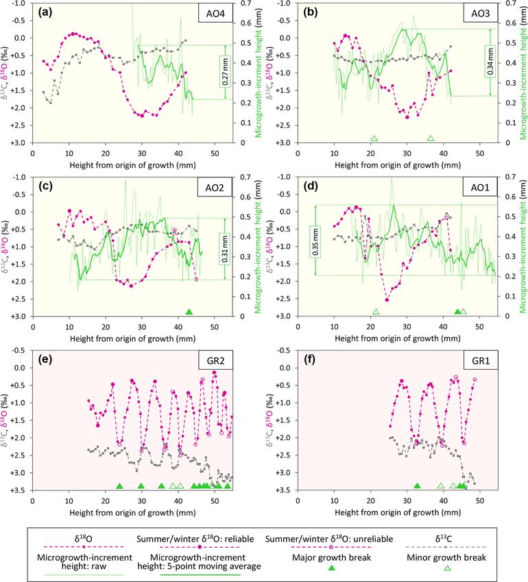
1204                                         A. L. A. Johnson et al.: Pliocene seasonality in the southern North Sea basin

warm interval before the change to the typically cooler-than-   tures in individual years over a late Pliocene interval span-
present conditions of the Pleistocene. During this interval,    ning the MPWP in Belgium and the Netherlands. The infor-
the Mid-Piacenzian Warm Period (MPWP; 3.28–3.03 Ma;             mation substantially supplements initial sclerochronological
Dowsett et al., 2019), “warm peak average” temperature was      estimates (Valentine et al., 2011) from these countries on the
2–3 ◦ C higher than now, similar to the GMST predicted for      eastern side of the southern North Sea basin (SNSB), and
the end of the present century (Dowsett et al., 2013). As       complements a sizeable body of equivalent data relating to
evident under current global warming, the mid-Piacenzian        the early Pliocene (Zanclean) sequence of eastern England,
temperature anomaly was not uniform, being for instance         on the western side of the SNSB (Johnson et al., 2009, 2021b;
greater than the global average figure at midlatitudes in the   Vignols et al., 2019). The results serve to (1) test estimates of
oceans according to results from both proxies and modelling     seasonality and annual (average) temperature obtained from
(Lunt et al., 2010). Despite general agreement, strong dis-     other proxies; (2) expand and refine the proxy evidence of
crepancies between proxy and model estimates of mean an-        temperature available for testing models of Pliocene climate;
nual sea surface temperature (ASST) have been identified in     (3) provide an insight into the controls on regional marine
some regions (Dowsett et al., 2011). Those formerly recog-      climate.
nized in the northern North Atlantic Ocean have been re-
duced by limiting proxy estimates to one source – alkenone
index – and adjusting model boundary conditions (Dowsett et
al., 2019). It is, however, widely considered (e.g. Robinson,   2   Sclerochronology and seasonality
2009; Bova et al., 2021) that alkenone index reflects temper-
ature in the warmer part of the year, and the same has now      The majority of sclerochronological studies of the environ-
been suggested to be the case for another commonly utilized     ment have been conducted on accretionary calcium carbon-
geochemical proxy, the Mg/Ca ratio of foraminiferal calcite     ate skeletons, principally those of corals and molluscs in the
(Bova et al., 2021). The species composition of assemblages     marine realm. Trace element (Sr/Ca) profiles from shallow-
of pelagic micro-organisms (particularly Foraminifera) has      water corals have been found to mirror seasonal changes in
been extensively used to derive both summer and winter          surface temperature (e.g. DeLong et al., 2007, 2011), but no
sea surface temperatures for the Pliocene (e.g. Dowsett et      such close relationship exists in molluscs (e.g. Gillikin et
al., 2010). The methodology, employing information on the       al., 2005; Markulin et al., 2019). In view of the absence of
seasonal temperatures associated with modern representa-        corals (at least long-lived, colonial forms) from extra-tropical
tives and relatives, assumes constancy of niche (“ecological    shallow-water environments and the general inutility of trace
uniformitarianism”; Vignols et al., 2019) and, furthermore,     (and minor) element data from molluscs for reconstructing
that both summer and winter temperatures exert an influence     seasonal temperature variation, sclerochronological investi-
on modern occurrence. This is questionable for the many         gations of palaeoseasonality in temperate and polar settings
forms that “bloom” in summer and those (dinoflagellates)        have been largely based on the δ 18 O of molluscan carbon-
that survive winter as cysts (dinocysts).                       ate. Pelagic belemnites supplement benthic molluscs as a
   It would be possible to obtain a more accurate estimate      provider of information on Jurassic and Cretaceous condi-
of regional mean ASST for comparison with model out-            tions (e.g. Mettam et al., 2014), but after the extinction of the
puts by combining temperatures from a summer proxy with         former at the end of the Cretaceous the latter become the sole
those from a winter proxy if such existed. Dearing Crampton-    source of data (e.g. Bice et al., 1996; Williams et al., 2010;
Flood et al. (2020) obtained TEX86 estimates about 6 ◦ C        Surge and Barrett, 2012; Johnson et al., 2009, 2017, 2019;
lower than from alkenones for sea temperature during the        Vignols et al., 2019; de Winter et al., 2020a, b). There is
MPWP in the Netherlands. They argued from several lines of      no doubt that temperature exerts an influence on the δ 18 O of
evidence that the former data reflect surface conditions dur-   molluscan carbonate, but values are also affected by the δ 18 O
ing winter, when the source organisms (archaea) of the lipids   of the fluid from which the material was precipitated (usually
concerned may have bloomed. Given that alkenones (pro-          taken to be equivalent to that of ambient water) and by kinetic
duced by haptophyte algae) seem to reflect summer surface       and more obscure “vital” effects (e.g. Owen et al., 2002a, b;
conditions, we could take the midpoint between the TEX86        Fenger et al., 2007; Garcia-March et al., 2011). At present it
and alkenone temperatures as an estimate of mean ASST.          is possible only to constrain (not specify) the δ 18 O of ambient
However, in the absence of information on the precise times     water in ancient settings, so, although precise, the tempera-
during winter and summer that are represented we could not      tures from δ 18 O thermometry are not necessarily accurate –
be sure of the accuracy of the mean ASST estimate, and we       i.e. they are questionable as absolute temperatures. Never-
would also be unable to say whether the winter and sum-         theless, assuming that kinetic and vital effects do not vary
mer figures give a full picture of seasonality. In this paper   with season or age, an assumption which is certainly valid
we use sclerochronology (investigation of the chemical and      for some molluscs (e.g. Fenger et al., 2007; Garcia-March
physical nature of accretionary mineralized skeletons) to ob-   et al., 2011), and that water δ 18 O is constant, ontogenetic
tain estimates of extreme summer and winter sea tempera-        profiles are, at least in principle, a true reflection of relative

Clim. Past, 18, 1203–1229, 2022                                                    https://doi.org/10.5194/cp-18-1203-2022
A. L. A. Johnson et al.: Pliocene seasonality in the southern North Sea basin                                                    1205

temperature and hence (from the difference between summer             equation of O’Neil et al. (1969) yields a seasonal temper-
and winter δ 18 O values) of seasonality.                             ature range of 7.8 ◦ C (summer 11.1 ◦ C, winter 3.3 ◦ C) and
   Unfortunately, molluscan growth is often discontinuous,            that of Kim and O’Neil (1997) a seasonal temperature range
and interruptions are frequently associated with seasonal             of 8.6 ◦ C (summer 8.8 ◦ C, winter 0.2 ◦ C). The differences in
temperature extremes (Schöne, 2008), so in such cases the             seasonal temperature range due to different water δ 18 O and
shell δ 18 O record does not fully reflect the range of tem-          absolute shell δ 18 O values are not great, but the differences
peratures experienced (e.g. Hickson et al., 2000; Peharda et          due to different equations are fairly significant for calcite (up
al., 2019a). However, because of their typical manifestation          to almost 1 ◦ C for the water and shell δ 18 O values specified
as “growth lines”, interruptions can be recognized and in-            above) and quite major for aragonite (over 3 ◦ C). Clearly,
stances of likely truncation of the δ 18 O record inferred (e.g.      therefore, the choice of equation must be given careful con-
Johnson et al., 2017, 2019, 2021b). The increasing occur-             sideration.
rence and/or duration of growth interruptions with age is part           Modelling (e.g. Williams et al., 2009) and carbonate
of the reason for the commonly observed reduction in am-              clumped isotope (147 ) analysis (e.g. Briard et al., 2020; Cal-
plitude of δ 18 O profiles through ontogeny, but general slow-        darescu et al., 2021) are techniques that have been used to
ing of growth (and consequent greater time averaging within           constrain water δ 18 O. The studies cited in relation to the lat-
samples) is also contributory (Goodwin et al., 2003; Ivany et         ter approach employ it to resolve seasonal fluctuations, and
al., 2003). Increasing sample resolution can potentially off-         de Winter et al. (2021) discuss the best sampling strategy
set this effect (Schöne, 2008), but the most accurate indica-         to achieve this end. In nearshore settings affected by major
tion of seasonal temperature variation is likely to be obtained       seasonal influxes of freshwater (normally isotopically light)
from early ontogenetic data (Goodwin et al., 2003; Ivany et           and which exhibit concomitant reductions in salinity, vari-
al., 2003). An exception to this rule is provided by Magal-           ation in water δ 18 O may be quite high. Lloyd (1964) doc-
lana (formerly Crassostrea) gigas, which exhibits substantial         umented change of more than 1 ‰ over a few months in
oxygen isotope disequilibrium in early ontogeny (Huyghe et            part of Florida Bay, and Ivany et al. (2004) inferred sea-
al., 2020, 2022).                                                     sonal variation of 2.5 ‰ in an Eocene nearshore setting in
   A problem as important as growth cessation/reduction for           the south-eastern USA. However, in more offshore settings
the inference of seasonal temperature range is the choice of          the effects of freshwater influx are much less. Thus in the
equation relating temperature to water and shell δ 18 O. Var-         modern North Sea seasonal variation in salinity is in most
ious equations exist for both aragonite and calcite, and for          places only 0.25 PSU (Howarth et al., 1993), which trans-
the same range in shell δ 18 O, these yield different tempera-        lates to a seasonal variation in water δ 18 O of just 0.07 ‰ us-
ture ranges. Thus for a water value of 0.0 ‰ and summer and           ing the salinity–water δ 18 O relationship for the North Sea of
winter shell values of 0.0 ‰ and +2.0 ‰, respectively, the            Harwood et al. (2008). Within a few tens of kilometres of
widely employed aragonite equation of Grossman and Ku                 the mouth of the Rhine seasonal variation in salinity rises
(1986) yields seasonal temperatures of 19.4 and 10.7 ◦ C –            to 0.75 PSU, and hence calculated variation in water δ 18 O
i.e. a seasonal range of 8.7 ◦ C. However, for the same δ 18 O        rises to 0.21 ‰ . At 20–30 m depth in the eastern part of the
values the Glycymeris glycymeris-specific aragonite equation          central North Sea, Schöne and Fiebig (2009) identified vari-
of Royer et al. (2013) yields seasonal temperatures of 17.4           ation in salinity of up to 2 PSU in certain years, which trans-
and 12.1 ◦ C – i.e. a seasonal range of only 5.3 ◦ C. Since both      lates to a variation in water δ 18 O of 0.55 ‰. If minimum and
equations are linear, like the LL (low-light) calcite equation        maximum water δ 18 O values differing by this amount coin-
of Bemis et al. (1998), used by Johnson et al. (2021b), neither       cided, respectively, with the times of maximum and mini-
the absolute values specifying a summer–winter difference of          mum water temperature, it would increase the temperature
2.0 ‰ in shell δ 18 O nor the value of water δ 18 O affect the cal-   range calculated from shell δ 18 O assuming constant water
culated seasonal temperature range. However, the non-linear           δ 18 O by an amount in the order of 2.6 ◦ C (figure for calcite
calcite equations of O’Neil et al. (1969; as reformulated by          using the LL equation mentioned above). However, the data
Shackleton et al., 1974) and Kim and O’Neil (1997) not only           of Schöne and Fiebig (2009) provide no evidence of a neg-
yield different temperature ranges for a given range in shell         ative correlation between salinity/water δ 18 O and tempera-
δ 18 O, but the temperature range in each case varies with the        ture, and near the eastern shore of the central North Sea there
absolute shell values concerned and with water δ 18 O. Thus           is a very strong positive correlation between water δ 18 O and
for a water value of 0.0 ‰ and summer and winter shell val-           temperature over the seasonal cycle (Ullmann et al., 2010; de
ues of 0.0 ‰ and +2.0 ‰, respectively, the calcite equation           Winter et al., 2021). This presumably reflects relatively high
of O’Neil et al. (1969) yields a seasonal temperature range of        evaporation in summer, combined with relatively low fresh-
8.2 ◦ C (summer 15.7 ◦ C, winter 7.5 ◦ C) and that of Kim and         water input, a common pattern in midlatitude settings and
O’Neil (1997) a seasonal temperature range of 8.9 ◦ C (sum-           one suggesting that seasonal variation in shell δ 18 O of ma-
mer 13.7 ◦ C, winter 4.8 ◦ C), but for a water value of +0.4 ‰        rine organisms at midlatitudes is more likely to be damped
and summer and winter shell values of +1.5 ‰ and +3.5 ‰               than enhanced by variation in water δ 18 O.
(i.e. the same 2.0 ‰ range but at higher absolute values), the

https://doi.org/10.5194/cp-18-1203-2022                                                          Clim. Past, 18, 1203–1229, 2022
1206 A. L. A. Johnson et al.: Pliocene seasonality in the southern North Sea basin
Even if there were a negative correlation between water mation, but the Piacenzian is better recorded in northern Bel-
δ 18 O and temperature, it would be confined to nearshore wa- gium by the Lillo Formation and in the south-west Nether-
ters (more susceptible to freshwater influx); hence the ef- lands by the Oosterhout Formation (Fig. 3). The last two
fect on calculated temperature range could be mitigated by formations essentially comprise marine sands, the Ooster-
the use of offshore shells. This approach introduces the pos- hout Formation at Ouwerkerk (Zeeland) probably having
sibility of underestimation of the surface range as a result been deposited in deeper water than the Lillo Formation at
of life positions below the summer thermocline (typically Antwerp from the evidence of fish otoliths (Gaemers and
at 25–30 m depth in shelf settings). However, shells from Schwarzhans, 1973) and a position farther from the inferred
sub-thermocline settings may be recognized from the asso- shoreline (Fig. 2). Nevertheless, Slupik et al. (2007) in-
ciated sediments and biota and, in the case of the scallop Ae- ferred a depth of deposition above storm wave base for most
quipecten opercularis, from microgrowth-increment patterns of the Oosterhout Formation at Schelphoek, 15 km north-
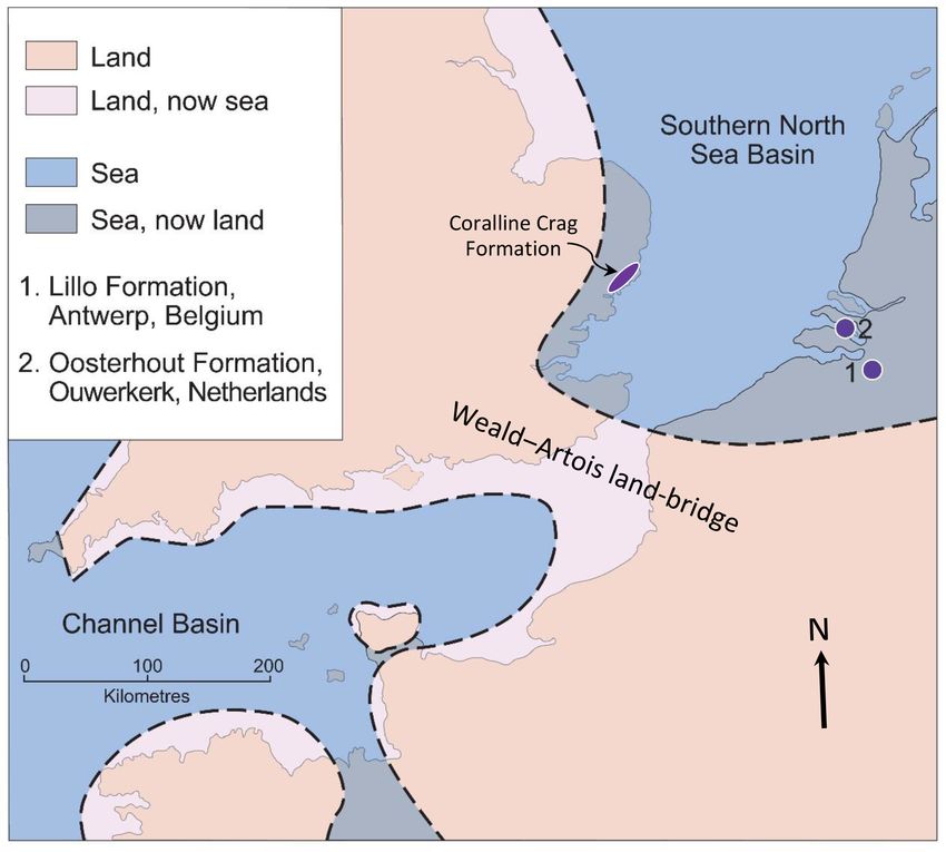
(Johnson et al., 2009, 2021b; Fig. 1). west of Ouwerkerk. In the Antwerp area depth estimates
While δ 18 O sclerochronology is potentially informative based on the fauna have varied between authors accord-
about seasonality, it should be clear from the foregoing that ing to the group studied, most of them hardly taking into
results from the technique need to be interpreted carefully. account the marked variation in sediment and sedimentary
The reliability of the information is of course also dependent structures within members of the Lillo Formation (see Deck-
on preservation of the original shell δ 18 O signature. Ivany ers et al., 2020, Figs. 4–6). According to Gaemers (1975),
and Judd (2022) provide a perspective on the issues consid- the otolith assemblage indicates a depth of at least 10–20 m
ered above and in addition present a mathematical approach for the “Kallo Sands” (Lillo Formation, Oorderen Member;
to reconstructing seasonality from the δ 18 O profiles of organ- Marquet and Herman, 2009) but less than 10 m for the over-
isms whose growth rate is not uniform. This is, however, de- lying Kruisschans Member. This indication of upward shal-
pendent on a strictly sinusoidal pattern of temperature vari- lowing is supported by assemblage evidence from dinocysts
ation over the year, which, as Ivany and Judd (2022) note, (Louwye et al., 2004; De Schepper et al., 2009), Foraminifera
cannot be assumed in sub-thermocline situations (i.e. in the (Laga, 1972), and bivalves (Marquet, 2004), but statistical
likely setting of some of the shells considered herein; see data from the last group suggest greater absolute depths: 35–
Sects. 3 and 5.3) 45 m for the Oorderen Member and 15–55 m for the Kruiss-
chans Member by the common overlap in depth range of
extant species; 40–50 m for the former and 20–50 m for the
3 Setting and material latter by the medial depth of extant species. The articulated
preservation of the semi-infaunal bivalve Atrina fragilis, lo-
In the Pliocene the marine area of the SNSB was some- cally in life position, within the Oorderen Member (Marquet
what greater than now (Fig. 2), partly due to higher global and Herman, 2009) is difficult to reconcile with the 10–20 m
sea level and partly to subsequent regional uplift (Westaway minimum depth estimate of Gaemers (1975), since speci-
et al., 2002). Onshore marine deposits exist to the west in mens would have been subject to fair-weather processes after
eastern England, and to the east in Belgium and the Nether- death. It is more likely that they lived at the depth suggested
lands, those in the last two countries passing eastwards into by Marquet (2004) and were killed by rapid burial (and per-
essentially fluvial non-marine deposits of the proto-Rhine– manently interred) in storms. A somewhat greater depth still
Meuse–Scheldt River system (Louwye et al., 2020; Mun- was inferred from the bivalve assemblage of the underlying
sterman et al., 2020). The Eridanos River system, drain- Luchtbal Member: 40–50 m by “common overlap”; 40–60 m
ing the Baltic area, had its exit into the SNSB in the area by “medial depth”. The low diversity of the bivalve fauna of
of the present German Bight, some 400 km north-east of the Merksem Member (overlying the Kruisschans Member)
the proto-Rhine–Meuse–Scheldt exit (Gibbard and Lewin, precluded the same statistical treatment, but Marquet and
2016). While at certain times a link may have existed be- Herman (2009) inferred from this impoverishment a depth of
tween the SNSB and the Channel Basin during the Pliocene less than 15 m, an estimate consistent with the foraminiferal
(either at the present position or across southern England; assemblage (Laga, 1972) and the high proportion of terres-
Funnell, 1996; Westaway et al., 2002; van Vliet-Lanoë et trial palynomorphs (De Schepper et al., 2009).
al., 2002; Gibbard and Lewin, 2016), at others the basins Dinocyst assemblages indicate surface temperatures
were separated by the Weald–Artois land bridge, as shown within the warm temperate range (but possibly only with re-
in Fig. 2. Water depth in the southern North Sea is now less spect to summer; Sect. 1) during the deposition of most of
than 40 m in most places but seismic stratigraphy indicates the Oorderen Member but punctuated by cool intervals and
that it was greater in the Pliocene, at least in areas of low preceded by continuously cool conditions during the depo-
sediment accumulation (Overeem et al., 2001). sition of the Luchtbal Member (De Schepper et al., 2009).
In eastern England there is a large stratigraphic gap be- The dinocysts of the Kruisschans and Merksem members
tween the Zanclean Coralline Crag Formation and the late mainly indicate a continuation of the warm conditions of
Piacenzian basal unit (“Walton Crag”) of the Red Crag For- the Oorderen Member but provide a few hints of cooling
Clim. Past, 18, 1203–1229, 2022 https://doi.org/10.5194/cp-18-1203-2022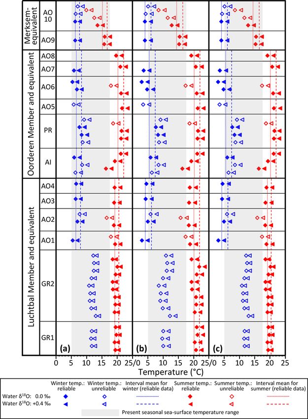
A. L. A. Johnson et al.: Pliocene seasonality in the southern North Sea basin                                                           1207

Figure 1. Pictorial demonstration of microgrowth-increment patterns in left valves of Aequipecten opercularis. (a) Typical supra-thermocline
specimen (mesotidal setting, 23 m depth, La Coruña, Galicia, Spain) showing small increments early and late in ontogeny. (b, c) Typical sub-
thermocline specimens (b microtidal setting, 50 m depth, Gulf of Tunis, Tunisia; c microtidal setting, 38 m depth, Adriatic Sea, Pula, Croatia)
showing large increments early in ontogeny. (d) Inferred sub-thermocline specimen (Ramsholt Member, Coralline Crag Formation, Broom
Pit, Suffolk, UK) showing large increments early in ontogeny and a transition from large to small increments late in ontogeny. Scale bars of
10 mm for whole-shell images (upper) and enlargements (lower). Major growth breaks (gb) identified in enlargements of (b, d). (a) University
of Derby, Geological Collections (UD) 53424; (b) National Museum of Natural History, Paris, IM-2008-1542 (one of seven specimens in
this lot); (c) UD 53423 (one of 48 specimens in this lot, coded S3A29); (d) UD 53425. See Johnson et al. (2009, 2021b) for numerical data
and discussion of microgrowth-increment patterns in A. opercularis. Modern supra-thermocline specimens show a difference of < 0.3 mm
between the maximum and minimum values of smoothed increment-height profiles, while the majority of sub-thermocline specimens show
a difference of > 0.3 mm.

(Louwye et al., 2004; De Schepper et al., 2009). Other ev-                for all species. Details of the provenance of the specimens
idence of this is provided by bivalves, fish, and pollen (Hac-            are given in Table 1, together with alphanumeric codes (AO:
quaert, 1960; Vandenberghe et al., 2000; Marquet, 2005), and              A. opercularis; AI: A. islandica; PR: P. rustica; GR: G. radi-
Wood et al. (1993) determined a 5–6 ◦ C decrease in summer                olyrata) and sundry basic descriptive information. Note that
surface temperature from the ostracods of a contemporane-                 the five specimens from the Oorderen Member sensu stricto
ous part of the Oosterhout Formation.                                     come from the Atrina fragilis bed, a horizon with the warm
   Previous sclerochronological investigation of late Pliocene            temperate dinocyst assemblage found at most levels in the
temperatures in Belgium and the Netherlands focussed on                   member. Illustrations of species other than A. opercularis
the Oorderen Member and an equivalent horizon in the Oost-                (Fig. 1) are provided in Fig. 4. Most, if not all, of the ma-
erhout Formation and was restricted to δ 18 O data from two               terial from the Lillo Formation was obtained from tempo-
bivalve species: Aequipecten opercularis and Atrina fragilis              rary exposures created during harbour works in the Antwerp
(Valentine et al., 2011). Here we supplement the existing                 area, while all the material from the Oosterhout Formation
δ 18 O data from A. opercularis with microgrowth-increment                was obtained from a borehole (Rijkswaterstaat-Deltadienst,
data from the same specimens to gain an insight into their hy-            afdeling Waterhuishouding, 42H19-4/42H0039) at Ouwerk-
drographic setting (sub- or supra-thermocline), and we also               erk, Zeeland. Interpretation of positions (depths) within the
supply δ 18 O data from two further bivalve species (Arctica              Ouwerkerk borehole in terms of members within the Lillo
islandica and Pygocardia rustica) from the Oorderen Mem-                  Formation follows Gaemers and Schwarzhans (1973) except
ber and another (Glycymeris radiolyrata) from the Lucht-                  in the case of AO8, for which we have accepted the opinion
bal Member. In addition, we provide A. opercularis data                   of Frank Wesselingh (in Valentine et al., 2011) that the po-
from the Luchtbal Member and horizons equivalent to the                   sition is equivalent to the Oorderen Member. Gaemers and
Luchtbal and Merksem members in the Oosterhout Forma-                     Schwarzans (1973) considered that strata of this age (Kallo
tion. Values for δ 13 C (obtained alongside δ 18 O) are reported          Sands) were missing at Ouwerkerk, but they appear to be

https://doi.org/10.5194/cp-18-1203-2022                                                                Clim. Past, 18, 1203–1229, 2022
1208                                               A. L. A. Johnson et al.: Pliocene seasonality in the southern North Sea basin

                                                                        from infaunal, slow-growing taxa to that derived from fast-
                                                                        growing, epifaunal A. opercularis, hence serving to mitigate
                                                                        any “ecological” bias in the results. We could not sample as
                                                                        many specimens of the infaunal, slow-growing species as of
                                                                        A. opercularis due to the limited availability of material (per-
                                                                        force from museums, in the lack of extant stratal exposures
                                                                        in the area of study). However, we sampled multiple years in
                                                                        the infaunal, slow-growing species, so the combined number
                                                                        of seasonal cycles investigated was similar to that in A. op-
                                                                        ercularis. We nevertheless expected some imbalance in the
                                                                        data because modern examples of Glycymeris species, from
                                                                        both cool- and warm-temperate settings, show winter cessa-
                                                                        tion or slowing of growth and thus supply (or would supply)
                                                                        underestimates of the seasonal temperature range from δ 18 O
                                                                        sclerochronology (Peharda et al., 2012, 2019a, b; Royer et
                                                                        al., 2013; Reynolds et al., 2017; Featherstone et al., 2020;
                                                                        Alexandroff et al., 2021). Various equations have been used
                                                                        to express the precise relationship between δ 18 O and tem-
                                                                        perature in modern Glycymeris (Royer et al., 2013; Peharda
Figure 2. Pliocene palaeogeography in the vicinity of the SNSB,         et al., 2019a, b), but species of this genus certainly exhibit
the location of sites in the Lillo (1) and Oosterhout (2) formations,   something at least close to equilibrium isotopic incorpora-
from which shells were obtained, and the area of onshore outcrop of     tion. The same is true of A. opercularis (Hickson et al., 1999;
the Coralline Crag Formation in eastern England (the partly Pleis-      Johnson et al., 2021b) and A. islandica (Schöne, 2013; Mette
tocene Red Crag Formation occurs over a larger area). Adapted           et al., 2018; Trofimova et al., 2018). Because of the simi-
from Valentine et al. (2011, Fig. 1), itself based on Murray (1992,     larity of δ 18 O values from seemingly well-preserved P. rus-
map NG1).
                                                                        tica from the Pliocene of Iceland to those from co-occurring,
                                                                        similarly preserved A. islandica (Buchardt and Simonarson,
                                                                        2003) it is reasonable to assume equilibrium fractionation in
well represented at Schelphoek, only 15 km away (Slupik et              the former (extinct) species. The specimens analysed showed
al., 2007).                                                             no physical signs of alteration, and they are unlikely to have
   According to the latest chronostratigraphy (Fig. 3), the             been heated by more than 10 ◦ C through burial as the thick-
material investigated is largely or entirely Piacenzian (3.60–          ness of overlying sediments was probably never much more
2.59 Ma) in age, the oldest (from the Luchtbal Member of                than 100 m (the depth below the present surface of the lower-
the Lillo Formation) being possibly as old as 3.71 Ma (latest           most shell from the Ouwerkerk borehole). Examples of both
Zanclean) and the youngest (from horizons in the Oosterhout             calcitic A. opercularis (including AO7 herein) and aragonitic
Formation equivalent to the Merksem Member of the Lillo                 A. fragilis from the Lillo Formation were shown by Valen-
Formation) being no younger than 2.76 Ma (De Schepper et                tine et al. (2011) to exhibit the original shell microstructure.
al., 2009). The MPWP is probably represented by material                Similarly good preservation has been demonstrated in a va-
from the Oorderen Member and the equivalent level in the                riety of calcitic and aragonitic species from the slightly ear-
Oosterhout Formation (Valentine et al., 2011). The Luchtbal             lier Ramsholt Member of the Coralline Crag Formation in
and Oorderen members are separated by an unconformity in-               eastern England (Johnson et al., 2009; Vignols et al., 2019).
terpreted by De Schepper et al. (2009) as a product of the sea-         We therefore considered it reasonable to proceed with iso-
level fall associated with Marine Isotope Stage (MIS) M2 (ca.           topic analysis of our material (both calcitic and aragonitic;
3.3 Ma), which marks a glacial episode. The Luchtbal Mem-               see Sect. 4 and Table 1) without detailed investigation of its
ber was therefore probably deposited before MIS M2 under                preservation. Moon et al. (2021) have recently shown that
interglacial conditions.                                                good mineralogical and microstructural preservation does
   All the specimens come from stratigraphic intervals with             not necessarily guarantee good preservation of original shell
a fully marine associated biota (e.g. Marquet, 2002, 2005;              δ 18 O. They heated shell material to 200 ◦ C and identified
Gaemers and Schwarzhans, 1973), in conformity with mod-                 consistent negative shifts in δ 18 O (1.5 ‰ after 2 weeks at this
ern occurrences in the case of the extant species A. opercu-            temperature) over an annual cycle but no significant miner-
laris and A. islandica (Tebble, 1976) and other fossil occur-           alogical or microstructural changes. As our specimens expe-
rences in the case of the extinct species P. rustica and G. ra-         rienced only minimal heating through burial, similar alter-
diolyrata (Norton, 1975; Buchardt and Simonarson, 2003;                 ation of shell δ 18 O is unlikely.
Marquet, 2002, 2005). Investigation of specimens of A. is-
landica, P. rustica, and G. radiolyrata added information

Clim. Past, 18, 1203–1229, 2022                                                            https://doi.org/10.5194/cp-18-1203-2022
Table 1. Basic information for the investigated specimens (all single valves). Order stratigraphic within formations (by member, then by borehole depth or bed, with entries for the
Oosterhout Formation inserted immediately above those, if any, for the equivalent member in the Lillo Formation). Entries in square brackets are interpretations (see footnotes). Latitudes
and longitudes are for the location indicated in the adjacent column and do not necessarily specify the exact place of collection (see Fig. 2 for the positions of Ouwerkerk and Antwerp).
UD: University of Derby, Geological Collections; IRSNB: Royal Belgian Institute of Natural Sciences, Brussels (MSNB was used for specimens discussed in Valentine et al., 2011).
Formation Member or Borehole depth Location Latitude, Genus and Repository Code Valve General Mineralogy Number of
equivalent (b-d) or bed longitude species and number herein height physical of sampled isotope
(in quotes) (mm) condition layer samples
Oosterhout “Merksem” b-d: 89.75–91 m Ouwerkerk 51.626◦ N, Aequipecten UD 53362 AO10 56 Incomplete Calcite 42
3.983◦ E opercularis
Oosterhout “Merksem” b-d: 93.5–94.5 m Ouwerkerk 51.626◦ N, Aequipecten UD 53363 AO9 46 Incomplete Calcite 30
3.983◦ E opercularis
https://doi.org/10.5194/cp-18-1203-2022
Oosterhout “Oorderen” b-d: 98.5–99.5 m Ouwerkerk 51.626◦ N, Aequipecten UD 53347 AO8 34 Incomplete, abraded Calcite 31
3.983◦ E opercularis
Lillo Oorderen Atrina fragilis bed Vrasenedok, 51.263◦ N, Aequipecten IRSNB AO7 42 Complete Calcite 31
Kallo, Antwerp 4.238◦ E opercularis Invert-29710-10
Lillo Oorderen Atrina fragilis bed Vrasenedok, 51.263◦ N, Aequipecten IRSNB AO6 51 Complete Calcite 39
Kallo, Antwerp 4.238◦ E opercularis Invert-29710-09
Lillo Oorderen Base Atrina fragilis bed Deurganckdok, 51.291◦ N, Aequipecten IRSNB AO5 31 Complete Calcite 23
Doel, Antwerp 4.257◦ E opercularis Invert-D2-8
Lillo Oorderen Atrina fragilis bed Vrasenedok, 51.263◦ N, Pygocardia IRSNB PR 62 Complete Aragonite 37
Kallo, Antwerp 4.238◦ E rustica Invert-29710-04
Lillo Oorderen Atrina fragilis bed [Antwerp]a 51.217◦ N, Arctica IRSNB AI 64 Complete Aragonite 32
4.421◦ E islandica Invert-18201-01
Aequipecten
A. L. A. Johnson et al.: Pliocene seasonality in the southern North Sea basin
Oosterhout “Luchtbal” b-d: 106–107.5 m Ouwerkerk 51.626◦ N, UD 53364 AO4 44 Incomplete, abraded Calcite 36
3.983◦ E opercularis
Lillo Luchtbal Palliolum gerardi bed Deurganckdok, 51.291◦ N, Aequipecten IRSNB AO3 42 Complete Calcite 28
Doel, Antwerp 4.257◦ E opercularis Invert-29710-13
Lillo Luchtbal Palliolum gerardi bed Deurganckdok, 51.291◦ N, Aequipecten IRSNB AO2 47 Complete Calcite 30
Doel, Antwerp 4.257◦ E opercularis Invert-29710-12
Lillo Luchtbal Palliolum gerardi bed Deurganckdok, 51.291◦ N, Aequipecten IRSNB AO1 54 Complete Calcite 28
Doel, Antwerp 4.257◦ E opercularis Invert-29710-11
Lillo Luchtbal [lower bed]b Deurganckdok, 51.291◦ N, Glycymeris IRSNB GR2 77 Broken in storage Aragonite 74
Doel, Antwerp 4.257◦ E radiolyrata 7698
Lillo Luchtbal [lower bed]b Deurganckdok, 51.291◦ N, Glycymeris IRSNB GR1 92 Broken in storage Aragonite 42
Doel, Antwerp 4.257◦ E radiolyrata Invert-29710-0062
a No specific location indicated within Belgium but highly likely to be Antwerp. b Species indicated as “special” to the lower bed of the Luchtbal Member in the Deurganckdok (Marquet, 2002).
Clim. Past, 18, 1203–1229, 2022
12091210 A. L. A. Johnson et al.: Pliocene seasonality in the southern North Sea basin
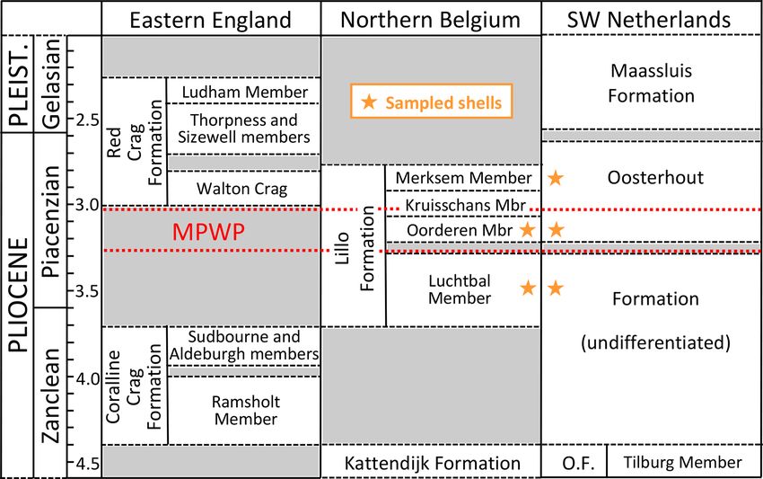
Figure 3. Stratigraphy and correlation of marine mid–late Pliocene and early Pleistocene units of the southern North Sea basin, with the
general stratigraphic positions of shells sampled for the present study (specific positions in Table 1). Age (Ma) of the Red Crag Formation and
constituent members (including the unofficial Walton Crag unit) according to Wood et al. (2009); of the Coralline Crag, Kattendijk and Lillo
formations and constituent members according to De Schepper et al. (2009) and Louwye and De Schepper (2010); and of the Oosterhout
(O.F.) and Maassluis formations according to Dearing Crampton-Flood et al. (2020) and Wesselingh et al. (2020). An additional small hiatus,
of uncertain age, is present in the lower part of the Oosterhout Formation (Dearing Crampton-Flood et al., 2020). The Maassluis Formation
includes a number of non-marine horizons (Slupik et al., 2007). Names of Lillo Formation members are in accordance with recent practice
(Louwye et al., 2020; Wesselingh et al., 2020), omitting “Sand”/“Sands”, as included by previous authors. Wesselingh et al. (2020) found
evidence of an additional layer (Broechem Unit) between the Kattendijk Formation and Luchtbal Member of the Lillo Formation. De Meuter
and Laga (1976) designated an additional, uppermost division of the latter formation (Zandvliet Member), but this may be no more than
the decalcified top of the Merksem Member (Louwye et al., 2020). Geographic provenance of shells and the location of the Coralline Crag
Formation are shown in Fig. 2. MPWP: Mid-Piacenzian Warm Period.
Figure 4. Right valves of (a) Arctica islandica, (b) Pygocardia rustica, and (c) Glycymeris radiolyrata from the Lillo Formation, Antwerp.
(a) Probably Oorderen Member, Verrebroekdok (IRSNB 7699); (b) Oorderen Member, Verrebroekdok (IRSNB 7700); (c) Luchtbal Member,
Deurganckdok (IRSNB 7701). Growth breaks are evident in all three specimens – e.g. ca. 10 major growth breaks in (b). Scale bar: 10 mm.
4 Methods with tap water and the shells then underwent the further
cleaning procedure adopted by Valentine et al. (2011) for
4.1 Laboratory procedures removal of any surficial organic matter, in preparation for
isotopic sampling of the outer shell layer from the exte-
The exterior of A. opercularis shells was coated with a sub- rior, as in other such investigations of A. opercularis (e.g.
limate of ammonium chloride and digitally photographed Hickson et al., 1999, 2000; Johnson et al., 2009, 2021b; Vi-
for the purpose of measuring microgrowth increments and gnols et al., 2019). The infaunal species were sampled in
the position of growth breaks. The coating was washed off
Clim. Past, 18, 1203–1229, 2022 https://doi.org/10.5194/cp-18-1203-2022A. L. A. Johnson et al.: Pliocene seasonality in the southern North Sea basin 1211 cross-section along the line of maximum growth, in accor- of growth meant that sampling had to start relatively far from dance with universal practice for A. islandica (e.g. Schöne et this point (minimum sample height 15.4 mm in GR2). al., 2005) and common practice for Glycymeris species (e.g. The cross-sections of the infaunal species were digitally Royer et al., 2013). For this purpose shells were stabilized in photographed for the purpose of measuring the positions of resin before sectioning – by the partial-encasement method sample holes and growth breaks, as seen on the shell exte- of Schöne et al. (2005) for A. islandica and P. rustica and rior (Fig. 4) and projected or traced (Fig. 5) into the isotope the total-encasement method of Johnson et al. (2021a) for sample path. Distances from the origin of growth were de- G. radiolyrata (fragments bonded beforehand). The use of termined from the images using the bespoke measuring soft- vacuum impregnation in the latter method resulted in resin ware Panopea (© 2004 Peinl and Schöne). Panopea was also penetration into the outer part of the outer shell layer. used to measure the position of growth breaks and the height Extraction of isotope samples from A. opercularis shells of microgrowth increments in the shell-exterior images of was by drilling a dorsal to ventral series of shallow com- A. opercularis (see Fig. 1). As in the case of isotope sample marginal grooves (depth and width < 1 mm; see Hickson et positions, measurements were made along the dorso-ventral al., 1999, their Fig. 2; 2000, their Fig. 3) in the external axis or (where this was impossible due to abrasion or encrus- surface, with the sample sites more closely spaced towards tation) lateral to this line, the measurements then being math- the ventral margin in an attempt to maintain temporal res- ematically adjusted as described by Johnson et al. (2019) to olution in the face of declining growth rate with age. De- correspond to ones made along the dorso-ventral axis. All tails of the procedure are given in Johnson et al. (2019) the microgrowth-increment measurements were made by the with respect to another scallop species. Mean sample spac- same person (Annemarie M. Valentine), thus assuring a rea- ing for individuals – the average distance between the centres sonably uniform approach given the subjective element in in- of grooves along the dorso-ventral (maximum-growth/shell- crement identification (Johnson et al., 2021b). Growth breaks height) axis – was 0.93 (AO8)–1.35 (AO9) mm. Sampling of were classified as major (incorporating “moderate”) or minor the infaunal species was by drilling a series of holes (depth in all species dependent on their external prominence (see and width < 1 mm; Fig. 5) in the outer shell layer as seen Figs. 1, 4). in cross-section, the curved path being located about mid- Samples (typically (50–100 µg) were analysed for their way between the external surface and the boundary between stable oxygen and carbon isotope composition (given as the outer and inner shell layers in A. islandica and P. rus- δ 18 O and δ 13 C) at the stable isotope facility, British Geo- tica but somewhat closer to the latter boundary in G. radi- logical Survey, Keyworth, UK (A. opercularis, A. islandica, olyrata to avoid resin-contaminated material (Fig. 5). Sample P. rustica), and the Institute of Geosciences, University of spacing was more constant than for A. opercularis, although Mainz, Germany (G. radiolyrata). At Keyworth, samples significantly reduced late in the long series from G. radi- were analysed using an Isoprime dual-inlet mass spectrom- olyrata GR2, again to maintain temporal resolution. Mean eter coupled to a Multiprep system; powder samples were sample spacing for individuals – the average distance be- dissolved with concentrated phosphoric acid in borosilicate tween the centres of holes, measured in terms of the dif- Wheaton vials at 90 ◦ C. At Mainz, samples were analysed ference in straight-line distance from the origin of growth using a Thermo Finnigan MAT 253 continuous-flow isotope – was 0.69 mm for A. islandica, 0.57 mm for P. rustica, and ratio mass spectrometer coupled to a Gasbench II; powder 0.54 mm (GR2) and 0.57 mm (GR1) for G. radiolyrata. Note samples were dissolved with water-free phosphoric acid in that in these relatively convex species the straight-line dis- helium-flushed borosilicate exetainers at 72 ◦ C. Both labo- tance from the origin of growth is not a measurement of shell ratories calculated δ 13 C and δ 18 O against VPDB and cali- height as normally defined (a distance from the umbo, which brated data against NBS-19 (preferred values: +1.95 ‰ for protrudes dorsally of the origin of growth in these forms; e.g. δ 13 C, −2.20 ‰ for δ 18 O) and their own Carrara Marble Fig. 5) and that the plane in which it was measured (along standard (Keyworth: +2.00 ‰ for δ 13 C, −1.73 ‰ for δ 18 O; the line of maximum growth) arguably does not include the Mainz: +2.01 ‰ for δ 13 C, −1.91 ‰ for δ 18 O). Values were shell-height axis in the prosogyrate species A. islandica and consistently within ±0.05 ‰ of the values for δ 18 O and P. rustica (dependent on the point at the shell margin that δ 13 C in NBS-19. This confirms the comparability of results is regarded as ventral). The lines of measurement and the from each laboratory established in earlier work (Johnson et values obtained are, however, regarded as “heights” for all al., 2019). Note that δ 18 O of shell aragonite was not corrected four species considered herein, for the sake of simplicity. for different acid-fractionation factors of aragonite and cal- The A. opercularis shells were relatively small (Table 1) and cite (for further explanation, see Füllenbach et al., 2015). were sampled from near the origin of growth (dorsal mar- gin) to a point at or close to the ventral margin (maximum 4.2 Calculation of temperatures sample height 53.0 mm in AO10). The shells of the infaunal species were larger (Table 1) and not sampled to the end of In previous work on late Pliocene bivalves from Belgium and ontogeny (maximum sample height 54.7 mm in GR2). Fur- the Netherlands, minimum and maximum estimates of global thermore, the thinness of the outer layer close to the origin average seawater δ 18 O (−0.5 ‰ and −0.2 ‰) and minimum https://doi.org/10.5194/cp-18-1203-2022 Clim. Past, 18, 1203–1229, 2022
1212                                              A. L. A. Johnson et al.: Pliocene seasonality in the southern North Sea basin

Figure 5. Cross-section of Glycymeris radiolyrata specimen GR2 showing the origin of growth (og), position of sample holes (relatively far
from the external surface in this species to avoid the darker, resin-contaminated material) and a major growth break (pale diagonal band in
enlargement) at shell height 35.4 mm. Scale bars: 10 mm. Black spot in enlargement is a marker to assist sample numbering.

and maximum modelled values for the early Pliocene in the               priate adjustments were made to allow for the different scales
western part of the SNSB (+0.1 ‰ and +0.5 ‰), all ad-                   used in measurement of water (VSMOW) and shell (VPDB)
justed downwards by 0.1 ‰ to allow for the input of isotopi-            δ 18 O values (Coplen et al., 1983; Vignols et al., 2019).
cally light freshwater into the eastern SNSB, were used to
calculate sets of temperatures from shell δ 18 O (Valentine et
                                                                        5   Basic results and analysis
al., 2011). It seems appropriate to apply the adjusted mod-
elled values more widely to late Pliocene material from Bel-            The isotopic, microgrowth-increment, and growth-break data
gium and the Netherlands. The adjusted global values are                are shown in Figs. 6 (Luchtbal Member and equivalent) and 7
probably unreasonably low (they supply implausibly cold                 (Oorderen Member and equivalent; Merksem Member equiv-
temperatures of 0.1 and 1.6 ◦ C, respectively, from AO6, a              alent). Read top to bottom, left to right (i.e. in the alphabet-
specimen from a horizon with a warm temperate dinocyst                  ical order of parts), the sequence in each figure is as in Ta-
assemblage) and are not used here.                                      ble 1, read top to bottom. The raw data are available online
   Valentine et al. (2011) employed the calcite equation of             (Johnson et al., 2021c).
O’Neil et al. (1969) for the calculation of temperatures from
A. opercularis, but there are grounds for thinking that this
provides slightly inaccurate figures (Hickson et al., 1999;             5.1 δ 18 O values and growth breaks
Vignols et al., 2019). The LL calcite equation of Bemis et              Apart from departures representing probable contamination
al. (1998) seems to provide more accurate figures (i.e. for             or “noise” (see Fig. 6d and caption), all profiles show cycli-
modern shells, a better fit with directly measured tempera-             cal patterns of δ 18 O variation, from less than half a cycle
tures) and certainly yields a larger estimate for seasonal range        in A. opercularis profiles starting near the origin of growth
(Johnson et al., 2021b). Both equations have therefore been             and terminating at a height of about 30 mm (AO8, AO5 –
employed herein to generate “minimum” and “maximum”                     Fig. 7c, f, respectively) to between two and three in a pro-
seasonal ranges from A. opercularis. Note that the calcite              file terminating at 53 mm (AO10 – Fig. 7a) but from be-
equation of Kim and O’Neil (1997) yields an intermediate                tween two and three cycles to substantially more over smaller
estimate, but the absolute temperatures obtained from mod-              height intervals in G. radiolyrata (between three and four
ern A. opercularis are too low (Johnson et al., 2021b).                 from 25-49 mm in GR1 – Fig. 6f; between eight and nine
   Just as there is some uncertainty as to the best equation for        from 15–55 mm in GR2 – Fig. 6e) and in P. rustica and A. is-
the calculation of temperatures from A. opercularis calcite,            landica (between two and three from 27–48 mm in each case
so different equations have been favoured for use with arag-            – Fig. 7g, h, respectively). In A. opercularis profiles extend-
onitic Glycymeris glycymeris. Royer at al. (2013) advocated             ing beyond one δ 18 O cycle, the amplitude commonly shows
the use of a species-specific equation developed by them,               a clear ontogenetic decrease. This pattern is less pervasive
while Reynolds et al. (2017) provide grounds for using the              and pronounced amongst the other species, and the A. is-
general aragonite equation of Grossman and Ku (1986). The               landica specimen shows an ontogenetic increase in ampli-
former yields a smaller estimate of seasonal range than the             tude. However, the lack of early ontogenetic data for com-
latter so again both have been employed herein in relation              parison from these species should be noted. The maximum
to G. radiolyrata. The equation of Grossman and Ku (1986)               amplitudes from G. radiolyrata specimens are less than from
is generally used in relation to aragonitic A. islandica and            most A. opercularis specimens, but those from P. rustica and
supplies similar temperatures from co-occurring (also arago-            A. islandica are similar to A. opercularis. Growth breaks,
nitic) P. rustica specimens (Buchardt and Simonarson, 2003).            albeit sometimes only minor, are associated with (< 1 mm
This, and no other equation, has therefore been used herein in          from the sample sites of) nearly all δ 18 O maxima and a few
relation to these species. In calculating temperatures appro-           δ 18 O minima from G. radiolyrata but with none of the max-

Clim. Past, 18, 1203–1229, 2022                                                             https://doi.org/10.5194/cp-18-1203-2022
A. L. A. Johnson et al.: Pliocene seasonality in the southern North Sea basin 1213
Figure 6. Ontogenetic profiles of δ 18 O, δ 13 C, and microgrowth-increment height from Luchtbal Member (and equivalent) A. opercularis (a–
d) and G. radiolyrata (e, f). Note that the isotopic axis has been reversed in each part such that lower values of δ 18 O (corresponding to higher
temperatures) plot towards the top. While the axis range is 4 ‰ throughout, the minimum and maximum values for A. opercularis (calcitic;
pale yellow background) have been set 0.5 ‰ lower than for G. radiolyrata (aragonitic; pale pink background) to facilitate comparison, given
the different fractionation factors applying for δ 18 O (Kim et al., 2007). The criteria for recognition of reliable and unreliable summer and
winter δ 18 O values are given in Sect. 6.1.1. The fairly large single-point δ 18 O excursion at height 18.5 mm in (d) is matched by a negative
one in δ 13 C and probably reflects contamination. Smaller interruptions of the large-scale cyclical pattern of δ 18 O variation in this and other
profiles represent “noise” (unexplained variability).
ima or minima from A. opercularis. Growth breaks are as- Taking the δ 18 O cycles to reflect seasonal temperature
sociated with two of the three maxima and two of the three variation and hence intervals of 1 year, the much smaller
minima from the A. islandica specimen and with two of the number over a given height interval from A. opercularis con-
three minima from the P. rustica specimen. firms that this species grew a great deal faster than the others
(more than twice as fast as A. islandica and P. rustica and
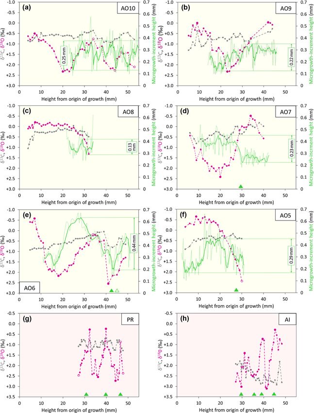
https://doi.org/10.5194/cp-18-1203-2022 Clim. Past, 18, 1203–1229, 20221214 A. L. A. Johnson et al.: Pliocene seasonality in the southern North Sea basin Figure 7. Isotopic, microgrowth-increment, and growth-break data from Merksem-equivalent A. opercularis (a, b) and Oorderen Member (and equivalent) A. opercularis (c–f), P. rustica (g), and A. islandica (h). Format and symbols as in Fig. 6. Clim. Past, 18, 1203–1229, 2022 https://doi.org/10.5194/cp-18-1203-2022
A. L. A. Johnson et al.: Pliocene seasonality in the southern North Sea basin 1215
3 to 5 times faster than G. radiolyrata). In A. opercularis means from early Pliocene A. opercularis (calcitic) and A. is-
profiles spanning 2 or more years (AO10, AO6 – Fig. 7a, e, landica (aragonitic) was ascribed principally to the miner-
respectively), there is an ontogenetic decrease in wavelength alogical difference (Vignols et al., 2019). This interpretation
as well as amplitude – i.e. growth was fastest in early on- is supported by the mean values from the present G. radi-
togeny. Ontogenetic decline in growth rate has been widely olyrata (aragonitic) specimens, which are similar to those
documented in A. opercularis from both δ 18 O and other ev- from A. islandica, but not by the P. rustica (also aragonitic)
idence (e.g. Johnson et al., 2021b), and in the present in- mean value, which is only a little outside the range of mean
stances (in which δ 18 O maxima and minima are not asso- values from A. opercularis. The different pattern of overall
ciated with growth breaks) the ontogenetic decrease in am- ontogenetic change in G. radiolyrata and A. islandica (in-
plitude of δ 18 O cycles is probably a consequence of the gen- crease, unlike in A. opercularis and P. rustica) also remains
eral slowing of growth with age, leading to time averaging to be explained, as does the unusual negative covariation be-
in samples. Whatever the explanation, seasonal temperature tween δ 13 C and δ 18 O in G. radiolyrata.
variation is likely to be most faithfully reflected by the first
δ 18 O cycle in A. opercularis profiles. The profiles from G. ra- 5.3 Microgrowth-increment patterns (A. opercularis)
diolyrata, P. rustica, and A. islandica undoubtedly omit sev-
eral early ontogenetic cycles and given the short wavelength Even in smoothed (five-point moving average) profiles of
of the later cycles represented, it may be that the amplitude microgrowth-increment size from A. opercularis, substan-
of these is reduced by time averaging, as inferred in A. oper- tial high-frequency variation is present in nearly all cases.
cularis. Even if the closer spacing of samples from G. radi- However, amongst those profiles long enough to show a low-
olyrata, P. rustica, and A. islandica may have been sufficient frequency pattern, in a number of cases a fairly clear and
in principle for the resolution of seasonal δ 18 O extremes, the complete major cycle proceeding from small to large to small
association of growth breaks with maxima, minima, or both increments is discernible over about the first 40 mm of shell
suggests that some recorded extremes are not representative height. Such a cycle is evident in three of the four Lucht-
of the most extreme temperatures experienced by the organ- bal Member (and equivalent) profiles, in each case with an
ism in the season concerned – i.e. δ 18 O variation may not amplitude (difference between the maximum and minimum
fully reflect seasonal temperature variation. of the smoothed profile) of more than 0.30 mm. The excep-
tion (AO4 – Fig. 5a) is a profile too short to show this pat-
tern. Only one (AO6 – Fig. 6g) of the four Oorderen Mem-
5.2 δ 13 C values ber (and equivalent) profiles has an amplitude greater than
Compared to δ 18 O values from the same specimen, δ 13 C 0.30 mm, but a second (AO5 – Fig. 6f) has an amplitude
values generally show much less variation, particularly only fractionally less and a third (AO8 – Fig. 6c) is too
within the span of δ 18 O cycles. Nevertheless, in some spec- short to show equivalent (“high-amplitude”) variation. De-
imens there are intervals exhibiting covariation between spite their considerable length the Merksem-equivalent pro-
δ 13 C and δ 18 O: moderate–strong positive covariation in files exhibit an amplitude well below 0.30 mm (“low ampli-
AO10 (Fig. 7a), AO6 (Fig. 7e), and PR (Fig. 7g) between tude”). The prevalent high-amplitude pattern from Luchtbal
shell heights 25 and 53 mm (r 2 = 0.61), 18 and 46 mm Member (and equivalent) shells corresponds to that in mod-
(r 2 = 0.84), and 31 and 46 mm (r 2 = 0.34), respectively; ern sub-thermocline shells, and the occurrence of the pattern
moderate–strong negative covariation in GR2 (Fig. 6e) and in an Oorderen Member shell is at least inconsistent with
GR1 (Fig. 6f) between shell heights 25 and 43 mm (r 2 = a supra-thermocline setting (Johnson et al., 2009, 2021b).
0.68) and 26 and 42 mm (r 2 = 0.40), respectively. However, The low-amplitude pattern in the two Merksem-equivalent
the general picture is of fluctuations (if any) in δ 13 C that are shells is consistent with a supra-thermocline setting; how-
independent of δ 18 O. The A. opercularis specimens show a ever, given the occasional occurrence of such a pattern in
marginal to clear overall decrease in δ 13 C through ontogeny, sub-thermocline shells, it is not inconsistent with the latter
while the P. rustica specimen shows little change and the setting.
A. islandica and G. radiolyrata specimens show clear overall
increases. The mean values from the A. opercularis speci- 6 Interpretation
mens are very similar – from +0.31 ± 0.22 ‰ (±1σ ) in AO8
to +0.77 ± 0.24 ‰ in AO9 – and comparable to the mean 6.1 Temperatures
from the P. rustica specimen (+0.98 ± 0.18 ‰) but much
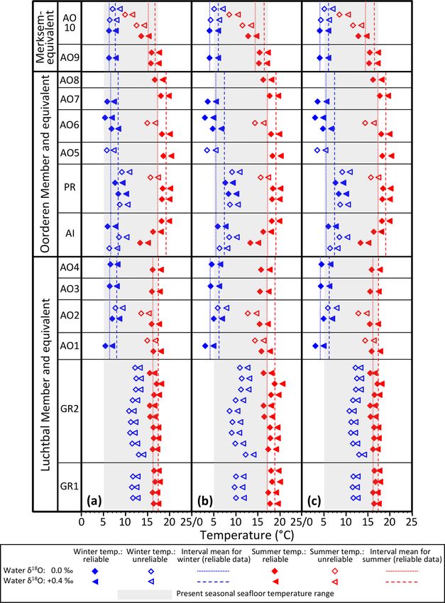
6.1.1 Derivation, comparison, and evaluation of
lower than the means from the A. islandica (+2.44±0.35 ‰)
seasonal seafloor values
and G. radiolyrata (GR1, +2.42 ± 0.40 ‰; GR2, +2.69 ±
0.32 ‰) specimens. The data from A. opercularis and A. is- The equations and water δ 18 O values that were employed to
landica compare closely with those from early Pliocene ex- calculate summer and winter temperatures from shell δ 18 O
amples of these species from eastern England (Johnson et are explained in Sect. 4.2. Following the reasoning of John-
al., 2009; Vignols et al., 2019). The difference between the son et al. (2017), the shell δ 18 O values used were the ex-
https://doi.org/10.5194/cp-18-1203-2022 Clim. Past, 18, 1203–1229, 2022You can also read