Guidelines on Ensemble Prediction System Postprocessing - 2021 edition - WMO-No. 1254
←
→
Page content transcription
If your browser does not render page correctly, please read the page content below
Guidelines on Ensemble Prediction
                        System Postprocessing

                        2021 edition
WEATHER CLIMATE WATER

                        WMO-No. 1254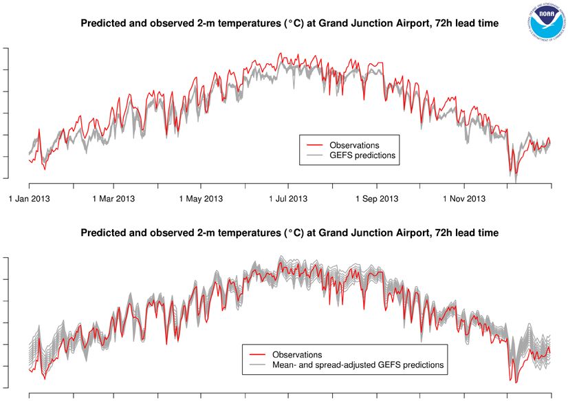
Guidelines on Ensemble Prediction
System Postprocessing

2021 edition

WMO-No. 1254
WMO-No. 1254

© World Meteorological Organization, 2021

The right of publication in print, electronic and any other form and in any language is reserved by
WMO. Short extracts from WMO publications may be reproduced without authorization, provided
that the complete source is clearly indicated. Editorial correspondence and requests to publish,
reproduce or translate this publication in part or in whole should be addressed to:

Chair, Publications Board
World Meteorological Organization (WMO)
7 bis, avenue de la Paix                                         Tel.: +41 (0) 22 730 84 03
P.O. Box 2300                                                    Fax: +41 (0) 22 730 81 17
CH-1211 Geneva 2, Switzerland                                    Email: publications@wmo.int
ISBN 978-92-63-11254-5
NOTE

The designations employed in WMO publications and the presentation of material in this publication do
not imply the expression of any opinion whatsoever on the part of WMO concerning the legal status of any
country, territory, city or area, or of its authorities, or concerning the delimitation of its frontiers or boundaries.

The mention of specific companies or products does not imply that they are endorsed or recommended by
WMO in preference to others of a similar nature which are not mentioned or advertised.
PUBLICATION REVISION TRACK RECORD

          Part/chapter/
   Date                   Purpose of amendment   Proposed by   Approved by
             section
CONTENTS
Page
ACKNOWLEDGEMENTS. . . . . . . . . . . . . . . . . . . . . . . . . . . . . . . . . . . . . . . . . . . . . . . . . . . . . . . . . . vii
EXECUTIVE SUMMARY. . . . . . . . . . . . . . . . . . . . . . . . . . . . . . . . . . . . . . . . . . . . . . . . . . . . . . . . . . . viii
KEY RECOMMENDATIONS. . . . . . . . . . . . . . . . . . . . . . . . . . . . . . . . . . . . . . . . . . . . . . . . . . . . . . . ix
CHAPTER 1. INTRODUCTION . . . . . . . . . . . . . . . . . . . . . . . . . . . . . . . . . . . . . . . . . . . . . . . . . . . . . 1
CHAPTER 2. PHYSICAL POSTPROCESSING . . . . . . . . . . . . . . . . . . . . . . . . . . . . . . . . . . . . . . . . . 5
2.1 Meteorological diagnostic information. . . . . . . . . . . . . . . . . . . . . . . . . . . . . . . . . . 5
2.2 Orographic downscaling (Tier 1). . . . . . . . . . . . . . . . . . . . . . . . . . . . . . . . . . . . . . . 7
CHAPTER 3. UNIVARIATE STATISTICAL POSTPROCESSING . . . . . . . . . . . . . . . . . . . . . . . . . . . 8
3.1 Deterministic bias correction (Tier 1) . . . . . . . . . . . . . . . . . . . . . . . . . . . . . . . . . . . 10
3.2 Deterministic model output statistics method (Tier 1). . . . . . . . . . . . . . . . . . . . . 12
3.3 Ensemble calibration methods . . . . . . . . . . . . . . . . . . . . . . . . . . . . . . . . . . . . . . . . 13
3.3.1 Ensemble model output statistics
(Tier 2 with site observations; Tier 3 on a grid) . . . . . . . . . . . . . . . . . . 13
3.3.2 Bayesian model averaging (Tier 2) . . . . . . . . . . . . . . . . . . . . . . . . . . . . 14
3.4 Quantile mapping (Tier 2) . . . . . . . . . . . . . . . . . . . . . . . . . . . . . . . . . . . . . . . . . . . . 15
3.5 Machine learning . . . . . . . . . . . . . . . . . . . . . . . . . . . . . . . . . . . . . . . . . . . . . . . . . . . . 16
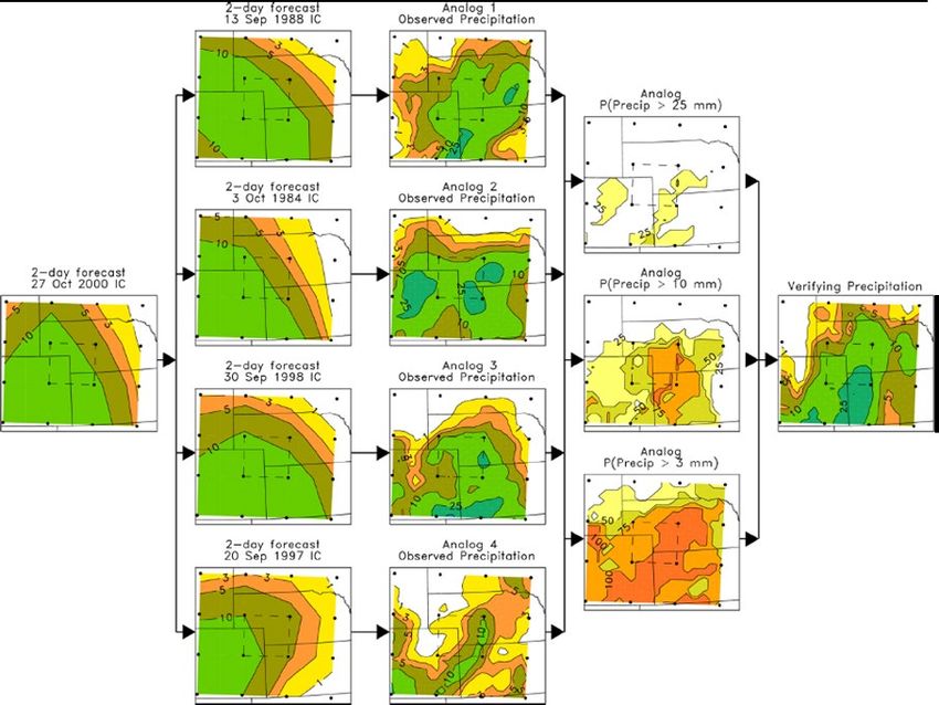
3.6 Analogue methods (Tier 3). . . . . . . . . . . . . . . . . . . . . . . . . . . . . . . . . . . . . . . . . . . . 17
3.7 Statistical downscaling using high-resolution
observations/analyses (Tier 3) . . . . . . . . . . . . . . . . . . . . . . . . . . . . . . . . . . . . . . . . . 19
3.8 Spatial methods – neighbourhood processing (Tier 2). . . . . . . . . . . . . . . . . . . . . 20
3.9 Extreme events . . . . . . . . . . . . . . . . . . . . . . . . . . . . . . . . . . . . . . . . . . . . . . . . . . . . . . 21
3.9.1 Extreme Forecast Index (Tier 3). . . . . . . . . . . . . . . . . . . . . . . . . . . . . . . 22
3.9.2 Point rainfall (Tier 3) . . . . . . . . . . . . . . . . . . . . . . . . . . . . . . . . . . . . . . . . 22
CHAPTER 4. MULTIVARIATE POSTPROCESSING. . . . . . . . . . . . . . . . . . . . . . . . . . . . . . . . . . . . . 24
4.1 Ensemble copula coupling (Tier 3) . . . . . . . . . . . . . . . . . . . . . . . . . . . . . . . . . . . . . 25
4.2 Blending of nowcasts and short-lead NWP forecasts (Tier 3). . . . . . . . . . . . . . . . 25
CHAPTER 5. MULTI-MODEL ENSEMBLES (TIER 3) . . . . . . . . . . . . . . . . . . . . . . . . . . . . . . . . . . . 28
CHAPTER 6. VERIFICATION AND VALIDATION. . . . . . . . . . . . . . . . . . . . . . . . . . . . . . . . . . . . . . 29
6.1 Validation best practice . . . . . . . . . . . . . . . . . . . . . . . . . . . . . . . . . . . . . . . . . . . . . . 29
6.2 Metrics for deterministic forecasts . . . . . . . . . . . . . . . . . . . . . . . . . . . . . . . . . . . . . 29
6.3 Metrics for probabilistic forecasts . . . . . . . . . . . . . . . . . . . . . . . . . . . . . . . . . . . . . . 29
6.3.1 Introduction. . . . . . . . . . . . . . . . . . . . . . . . . . . . . . . . . . . . . . . . . . . . . . . 29
6.3.2 Methodology of verification . . . . . . . . . . . . . . . . . . . . . . . . . . . . . . . . . 30
6.3.3 Continuous ranked probability score . . . . . . . . . . . . . . . . . . . . . . . . . . 32
CHAPTER 7. DATA INFORMATION. . . . . . . . . . . . . . . . . . . . . . . . . . . . . . . . . . . . . . . . . . . . . . . . . 33
7.1 Data-science considerations: the bias-variance trade-off . . . . . . . . . . . . . . . . . . . 33
7.2 Data management considerations. . . . . . . . . . . . . . . . . . . . . . . . . . . . . . . . . . . . . . 33
7.3 Basic data characteristics of ensemble forecasts . . . . . . . . . . . . . . . . . . . . . . . . . . 35
7.3.1 Lagged ensembles . . . . . . . . . . . . . . . . . . . . . . . . . . . . . . . . . . . . . . . . . 35
7.3.2 Multi-model ensemble combinations . . . . . . . . . . . . . . . . . . . . . . . . . 35
7.4 Use of and need for reforecasts for calibration . . . . . . . . . . . . . . . . . . . . . . . . . . . 36
CHAPTER 8. SOFTWARE AND TECHNICAL INFORMATION . . . . . . . . . . . . . . . . . . . . . . . . . . . 37
8.1 Data sources . . . . . . . . . . . . . . . . . . . . . . . . . . . . . . . . . . . . . . . . . . . . . . . . . . . . . . . . 37
8.2 Computing platforms . . . . . . . . . . . . . . . . . . . . . . . . . . . . . . . . . . . . . . . . . . . . . . . . 37
8.3 R packages . . . . . . . . . . . . . . . . . . . . . . . . . . . . . . . . . . . . . . . . . . . . . . . . . . . . . . . . . 37
8.4 Python libraries . . . . . . . . . . . . . . . . . . . . . . . . . . . . . . . . . . . . . . . . . . . . . . . . . . . . . 37
8.5 GrADS. . . . . . . . . . . . . . . . . . . . . . . . . . . . . . . . . . . . . . . . . . . . . . . . . . . . . . . . . . . . . . 38vi GUIDELINES ON ENSEMBLE PREDICTION SYSTEM POSTPROCESSING
Page
LIST OF ACRONYMS . . . . . . . . . . . . . . . . . . . . . . . . . . . . . . . . . . . . . . . . . . . . . . . . . . . . . . . . . . . . . 39
REFERENCES. . . . . . . . . . . . . . . . . . . . . . . . . . . . . . . . . . . . . . . . . . . . . . . . . . . . . . . . . . . . . . . . . . . . 40ACKNOWLEDGEMENTS This publication was prepared by the WMO Commission for Observation, Infrastructure and Information Systems (INFCOM) Standing Committee on Data Processing for Applied Earth System Modelling and Prediction (SC-ESMP) through concerted efforts by the following authors: Ken MYLNE, Met Office, United Kingdom of Great Britain and Northern Ireland Jing CHEN, China Meteorological Administration, China Amin ERFANI, Meteorological Service of Canada, Canada Tom HAMILL, National Oceanic and Atmospheric Administration (NOAA), United States of America David RICHARDSON, European Centre for Medium-Range Weather Forecasts (ECMWF) Stéphane VANNITSEM, Royal Meteorological Institute of Belgium, Belgium Yong WANG, Central Institute of Meteorology and Geodynamics (ZAMG), Austria Yuejian ZHU, National Oceanic and Atmospheric Administration, USA This publication was reviewed by: Hamza Athumani KABELWA, Tanzania Meteorological Agency, United Republic of Tanzania Stephanie LANDMAN, South African Weather Service, South Africa Eunha LIM, WMO Jianjie WANG, China Meteorological Administration, China The following individuals also provided valuable contributions to this publication: Aitor ATENCIA, ZAMG, Austria Markus DABERNIG, ZAMG, Austria
EXECUTIVE SUMMARY

The present guidelines on ensemble prediction system (EPS) postprocessing describe various
postprocessing methods by which WMO Members can use information from available EPS
forecasts to enhance and improve forecasts for their own specific regions or areas. They provide
background on which statistical methods and data choices may be used for training, real-time
forecasting, and validation. This publication is not a comprehensive instruction manual on how
to implement methods or an explanation of the detailed mathematics behind the methods used;
however, wherever possible, it provides references to where such information can be found.
References to where available postprocessing software can be found are also provided.

These guidelines cover aspects of both physical and statistical postprocessing and take into
consideration the opportunities offered by data science methods. With respect to physical
postprocessing, a number of aspects are examined, including meteorological diagnosis and
orographic downscaling. For statistical postprocessing, issues covered include bias correction,
deterministic model output statistics, and ensemble calibration. The use of verification
techniques to test and validate the postprocessing of both deterministic and probabilistic (EPS)
forecasts is also discussed.

The present guidelines propose that WMO Members access real-time forecast data, historical
data and reforecast data sets from the WMO Global Data-processing and Forecasting
System (GDPFS). Obtaining data from GDPFS is much more cost-effective for Members
than independently operating their own numerical weather prediction (NWP) systems.
Postprocessing can greatly enhance the accuracy of real-time forecast data for applications at
relatively low cost. The development of many of the postprocessing methods requires access to
historical and reforecast data, both for statistical training and for validation purposes.
                                               ix

KEY RECOMMENDATIONS

1.   Statistical postprocessing has consistently been demonstrated to improve the quality of
     both ensemble and deterministic forecasts and is one of the most cost-effective ways to
     produce higher-quality products. It is recommended that National Meteorological and
     Hydrological Services (NMHSs) utilize these postprocessing methods to enhance their
     forecasting capabilities.

2.   NMHSs can apply postprocessing methods to model data which are available from existing
     prediction centres at a minimal cost relative to the cost required to operate an NWP system.
     It is therefore strongly recommended that NMHSs leverage data from WMO-designated
     GDPFS centres (see Section 8.1).

3.   An archive of quality-controlled observations and past forecasts is essential for the
     training of statistical postprocessing and data science techniques and for validation
     and verification purposes. It is recommended that NMHSs continue to archive local
     data and, where possible, that they share these data with Regional Specialized
     Meteorological Centres (RSMCs) and global centres for statistical adaptation and model
     calibration purposes.

4.   When beginning to apply postprocessing methods, it is recommended that NMHSs
     start with simple variables, such as surface temperature, and with data from their own
     local stations, rather than gridded data (which require greater storage and computation
     capabilities).

5.   For deterministic forecasts of easier variables, it is recommended that NMHSs start by using
     the decaying average bias correction method, also referred to as the Kalman filter-type
     method (see Section 3.1). For ensemble forecasts, it is recommended that NMHSs start by
     using the ensemble model output statistics (EMOS) method (see Section 3.3.1).

6.   It is essential that NMHSs use best practices in the development of their postprocessing
     methods. These practices include separating training and validation data and verifying
     both the original and the postprocessed forecasts against the validation data using
     a number of metrics (for example, continuous ranked probability skill score (CRPSS),
     reliability) and by comparing a visualization of the forecast with the verifying observations.
     (Ideally, this should be done by independent forecasters). Languages such as R and Python,
     for which there are many available software packages, can aid in the development of
     postprocessing methods (see Section 8.3 and Section 8.4).

7.   In order to construct an operational forecasting system, NMHSs must have the ability to
     periodically obtain model and observation/analysis data for training and validation. In
     addition, NMHSs must have the capability to develop appropriate postprocessing methods
     and must be able to display and validate the products of those methods. Implementing
     and maintaining a comprehensive operational forecasting system will entail a significant
     investment of time, resources and effort.
CHAPTER 1. INTRODUCTION Numerical weather prediction (NWP) involves the use of mathematical models capable of simulating the atmosphere to forecast the development of the weather over the next several days. Models are initialized using an analysis of the current state of the atmosphere generated from the most recent observations through a process called data assimilation. There are two standard forms of NWP: the older deterministic method, and the newer ensemble prediction system (EPS) method. The deterministic method is still widely employed today and generates a single model forecast. The problem with deterministic forecasts, however, is that they provide no information on the confidence or uncertainty in a forecast. Sometimes, for example, a forecast can go badly wrong very quickly and the forecaster or user has no warning of this. An EPS, in contrast, runs the model many times instead of just once. Each forecast within an ensemble is referred to as an ensemble member, and the members are initiated from very slightly different versions of the analysis. If all the members evolve similarly, this provides high confidence in the forecast. If, however, the various members diverge from each other, this indicates less confidence in the forecast, with the ensemble providing an estimate of the probabilities of different outcomes. EPSs are therefore generally used to provide probabilistic forecasts and to support risk-based forecasts and warnings. EPSs have become a powerful tool for forecasting weather and its uncertainty across the globe and underpin severe weather warnings intended to protect life and property. Developing, operating and regularly improving modern EPSs capable of producing high-quality data is extremely expensive. By comparison, postprocessing systems which enhance the quality of EPS forecasts are much more economical to develop and apply and can result in improvements in the skill of EPS forecasts equivalent to many years of EPS system upgrades, particularly for local weather forecasts. A number of Global Data-processing and Forecasting System (GDPFS) centres designated by WMO as World Meteorological Centres (WMCs) or Regional Specialized Meteorological Centres (RSMCs) make NWP data (from both EPSs and individual deterministic models) available for use and postprocessing by WMO Members. Even for National Meteorological and Hydrological Services (NMHSs) with their own EPS or deterministic NWP systems, investing in postprocessing systems will greatly enhance the quality and usefulness of their forecasts. These guidelines provide an overview of those postprocessing methods which have been proven to be effective. Although the focus is on EPSs, some simple deterministic postprocessing is also included as a starting point and to aid in understanding. This publication does not provide a full documentation of postprocessing methods or a step-by-step guide to their implementation; however, it does provide references for further details. Two particular books are especially recommended in this regard: Statistical Postprocessing of Ensemble Forecasts, by S. Vannitsem, D.S. Wilks and J.K. Messner and Statistical Methods in the Atmospheric Sciences by D.S. Wilks (see the References section for full bibliographic details). Postprocessing methods range from the relatively simple to the highly complex, and the computing resources, data and technical expertise of the staff required to develop and implement these methods are variable. In order to help WMO Members select the methods most suitable for their needs, capabilities and resources, each method described is allocated to one of the three tiers outlined in Table 1. In general, it is recommended that NMHSs should start by implementing a method corresponding to the complexity, requirements and limitations indicated for Tier 1. These methods are some of the simplest postprocessing methods and can produce substantial benefits while requiring relatively little investment. NMHSs can then progress to the more advanced methods described in Tiers 2 and 3 as requirements and resources allow.
2                       GUIDELINES ON ENSEMBLE PREDICTION SYSTEM POSTPROCESSING

    Table 1. Breakdown of postprocessing methods according to complexity, requirements and
                                          limitations

     Tier       Scientific and       Technical implementation       Data requirements          Limitations
                mathematical          complexity and resource
                 complexity                  demands
Tier 1      Conceptually             May be implemented at        Access to basic EPS     Univariate
            intuitive systems and    a basic level on a desktop   (and individual         improvements may
            basic university-level   PC; standard software        deterministic           lose consistency or
            mathematics              likely to be available and   model) outputs          covariances; may
                                     implemented without          and observations or     degrade forecasts
                                     specialist software          analyses with a short   of rare or extreme
                                     engineering skills           historical record       events
                                                                  (≤1 year); typically,
                                                                  single-site, rather
                                                                  than gridded data
                                                                  sets
Tier 2      Moderate                 Requires a                   Access to gridded       Risk of over-fitting
            complexity,              high-powered desktop         EPS fields and/or long to rare and extreme
            possibly involving       PC or larger computer,       archive records of site events
            multivariate             high-bandwidth data          data amounting to
            inputs and some          connectivity and the         many Mbytes (up to
            performance              ability to process large     one Gbyte); complex
            optimization             (Gbyte) data sets            data handling to
            requiring scientific                                  match observations
            testing skills before                                 to forecasts (for
            implementation                                        example, large
                                                                  databases)
Tier 3      Advanced                 Requires                     May require very        Challenging to write
            mathematical             high-performance             large data sets or      algorithms and to
            methods and/             computing installation       long time series of     put into operation
            or detailed              and expert software          data for training
            meteorological           engineering skills to
            understanding            implement operationally
            required                 or for real-time
                                     prediction; may require
                                     access to large “big
                                     data” archives (many
                                     Gbytes) with high
                                     connectivity

This table is intended to provide a general overview of the various tiers of postprocessing
methods. Not all methods will clearly fit into a particular tier. For example, a certain method
might meet the requirements for Tier 1 but might require Tier 2-level computational capabilities
if applied to large numbers of sites or high-resolution gridded data. In general, a method will
be categorized according to its highest demand with respect to its scientific, technical and data
requirements.

Table 2, below, presents a specific example of the breakdown of the Kalman filter model output
statistics (MOS) postprocessing method. The Kalman filter MOS postprocessing method is a Tier
1 method because its complexities, data requirements and limitations are consistent with those
described in the Tier 1 category in Table 1. Throughout these guidelines, when a postprocessing
method is introduced, the tier to which it corresponds will be indicated in bold.
CHAPTER 1. INTRODUCTION 3
Table 2. Example of the complexities, requirements and limitations of the Kalman filter
MOS method
Tier Scientific and Technical Data requirements Limitations
mathematical implementation
complexity complexity and
resource demands
Tier 1 Kalman filter MOS Standard Python Site forecasts provided from May degrade
method for bias or R code from an EPS centre for a small extreme forecasts
correction of site software library number of sites on a daily
forecasts using site implemented on basis and received over a low
observations a PC bandwidth connection; site
observations from a local
archive updated daily
Chapter 2 in this publication describes simple postprocessing techniques which can add
significant benefits in terms of increasing the accuracy of a forecast. These techniques include
calculating additional diagnostics from a small number of model output variables based on
a physical understanding of the geography and atmospheric conditions, selecting the most
relevant values for a location from model grid values according to factors such as coastlines and
land elevation, and adjusting the model values to account for elevation using simple physical
laws. These techniques can be applied equally to deterministic model outputs or to each
member of an EPS.
Where a set of past forecasts and observations is available for one or more locations and
where errors are Gaussian-distributed and relatively consistent across samples, simple bias
corrections or regression relations can be derived to correct systematic errors. However, more
involved techniques are typically needed for elements such as heavy precipitation amount or
precipitation type. Statistical methods which are designed to improve the quality of forecasts of
a specific element of the weather are called “univariate”, and candidate univariate techniques
for both deterministic forecasts and full ensemble probability distributions are briefly described
in Chapter 3.
Both EPSs and individual deterministic models provide gridded scenarios where many elements
of the weather are physically consistent with other elements, both temporally and spatially.
However, many univariate calibration methods do not take this consistency into account. For
some applications, these covariances are important, and multivariate techniques which do
account for physical consistencies among elements are described in Chapter 4.
Chapter 5 provides some brief guidance on suitable approaches to use with multi-model
ensembles if one synthesized forecast is desired.
It is essential that forecasts be verified and validated in order to allow end users to obtain
quantitative and qualitative information regarding forecast skill and to ensure that
postprocessing methods are improving forecast accuracy as expected. Chapter 6 provides some
background on common verification metrics and the best practices to follow when constructing
a verification system. Key reference material includes the Australian website
https://www.cawcr.gov.au/projects/verification/, the contents of which were developed by the
WMO Joint Working Group on Forecast Verification Research and books by Wilks (2019) and
Jolliffe and Stephenson (2012).
Chapter 7 discusses general issues concerning data handling and computational requirements.
Statistical postprocessing methods depend on the availability of high-quality data, and this
chapter reviews some of the issues which can be expected when obtaining and maintaining
training and validation data. While it has been a common experience that short-lead forecasts of
variables such as surface temperature can be improved using a relatively short time series of past
forecasts and observations, both longer-lead forecasts and forecasts of more extreme events,
such as heavy precipitation, may benefit from longer training data sets and data from more than4 GUIDELINES ON ENSEMBLE PREDICTION SYSTEM POSTPROCESSING one prediction system. Long-lead forecasts and extreme event forecasts are both in demand, the former to provide more lead time to make decisions and the latter because of the much greater societal impact of extreme events. Chapter 8 contains technical information, such as where to obtain the software and data necessary to build or improve postprocessing systems.
CHAPTER 2. PHYSICAL POSTPROCESSING

An NWP model uses the principles of dynamics and physics in relation to the atmosphere
to make predictions about weather. Depending on the model’s horizontal grid spacing and
number of vertical levels, it may not fully resolve all atmospheric processes at the grid scale. If
this is the case, the NWP model needs to use physical parameterizations, such as condensation
and convective schemes, at the sub-grid scale to fill in the gap. However, in some situations,
even with the most sophisticated parameterization schemes, some of the finer details of the
atmosphere are not predicted well. Examples include the mode and severity of convective storms
and the partitioning between the various phases of the precipitation. In addition, because
the model’s surface data depends partly on the atmosphere, if the atmospheric processes are
not fully resolved, over areas with complex topography, the model’s surface data may not
be sufficiently precise. In these situations, physical postprocessing of the direct model data
can add extra details to or improve the quality of the forecast. In this chapter, some physical
postprocessing methods are discussed. All these methods assume an unbiased model input.
Although these methods are explained in terms of deterministic models, they can be applied to
all members of an EPS. Once a range of values is obtained, these values can then be put into a
probabilistic context using statistical methods.

2.1          Meteorological diagnostic information

The meteorological diagnostic information presented in this section can be calculated using
methods involving prognostic variables (temperature, humidity, wind speed and direction) that
are output from operational NWP models.

1)    The following diagnostic information concerns the impact of ambient temperature,
      humidity and wind on human well-being.

      a.   HUMIDEX (Materson and Richardson, 1979): A dimensionless number representing
           the level of discomfort people feel that is attributable to humidity during hot days.
           It is calculated based on the temperature and partial vapor pressure of the ambient
           air. (Tier 1)

      b.   Wind chill index (Osczevski and Bluestein, 2005): The combined effect of wind and
           low temperature (below freezing) on how cold the ambient air feels on human skin
           (see Figure 1). (Tier 1)

2)    The following diagnostic information concerns the severity of the convective storms
      that an environment can produce. It is calculated based on the available instability and
      wind shear data.

      a.   Lifted index (Galway, 1956) is calculated based on the difference between the
           temperature of an air parcel lifted from near surface to 500 hPa and the corresponding
           environmental temperature. (Tier 1/Tier 2*)

      b.   Showalter index (Showalter, 1953) is calculated based on the difference between the
           temperature of an air parcel lifted from 850 hPa to 500 hPa and the corresponding
           environmental temperature. (Tier 1/Tier 2*)

      c.   Severe Weather Threat (SWEAT) index (Djurik, 1994) is calculated based on the low
           to mid-level wind and temperature. (Tier 1/Tier 2*)

      d.   Total Total index (Djurik, 1994) is calculated based on the low to mid-level
           temperature. (Tier 1/Tier 2*)

      e.   George’s K-index (George, 1960) is calculated based on the low to mid-level
           temperature and dewpoint temperature. (Tier 1/Tier 2*)
6 GUIDELINES ON ENSEMBLE PREDICTION SYSTEM POSTPROCESSING
Wind chill temperature (°C)
0 –5 –10 –15 –20 –25 –30 –35 –40 –45
2
4
6
Wind speed (m/s)
8
10 Very cold
12
Danger of frostbite
14
16
Great danger
of frostbite
18
20
–25 –35 –60
Wind chill index (°C)
Figure 1. Example of the variation of the wind chill index with respect to temperature and
wind speed
Source: https://en.wikipedia.org/wiki/ Wind _chill#/media/File:Windchill_effect _en.svg
f. Storm Relative Helicity index (Thompson, 2006) is an index that gives information
on the low-level environmental wind shear, taking into account both wind speed and
wind direction. (Tier 1/Tier 2*)
g. Convective Available Potential Energy (CAPE) (Markowski and Richardson, 2010)
is the theoretical maximum energy available to a convective storm. Conceptually, it
is proportional to the kinetic energy that a parcel can gain from its environment as a
result of positive buoyancy. This parameter is usually available as a direct NWP output.
(Tier 1/Tier 2*)
h. Convective Inhibition (CIN) (Mapes, 1999) refers to a negative buoyant energy
that will inhibit the convection from occurring. Conceptually, it is the opposite of
CAPE. The presence of CIN in most cases is at the lower part of the atmosphere.
(Tier 1/Tier 2*)
* The above diagnostic information is classified as Tier 1 if it is provided as an NWP model
output. If it is not provided as an NWP model output, and instead requires data from multiple
vertical levels within the NWP model, it is classified as Tier 2.
3) Most existing operational NWP models have condensation schemes that can only
produce liquid and solid precipitation as direct model outputs. To obtain mixed-phase
precipitation, some diagnostic methods (Bourgouin, 2000; Scheuerer et al., 2016) are
used. The calculations for these methods are usually done within the model, but they can
be postprocessed outside of the model. They are usually based on model’s environmental
temperature and assume unbiased input. Diagnostic methods for calculating mixed-phase
precipitation are classified as Tier 1 if they are carried out within an NWP model with
precipitation types presented as model outputs. However, if methods for calculating
mixed-phase precipitation are carried out outside of an NWP model, they require data on
multiple model levels and are classified as Tier 2.CHAPTER 2. PHYSICAL POSTPROCESSING 7 2.2 Orographic downscaling (Tier 1) The surface fields, such as the surface temperature, of a model at a point m1 can be projected over a given region at a corresponding point m2. Depending on the resolution of the model, a direct interpolation may cause a misrepresentation in the continuity of the field once several other neighbouring points are projected. This occurs in particular over areas of complex topography due to height variations between the model topography and the actual region. Postprocessing can be used to downscale the surface temperature, for example, by using a standard lapse rate of L=6.5 °C/km (or the model environmental lapse rate when available) to estimate the temperature difference between points m1 and m2 and then by adding or subtracting the correction to the field at m2. This is done by simply defining the height difference between m1 and m2 and then multiplying this difference by L. The same technique can be used for the neighbouring points. The resulting output is an adapted and continuous model surface temperature projected over the needed region.
CHAPTER 3. UNIVARIATE STATISTICAL POSTPROCESSING
Because statistical postprocessing can dramatically improve the quality of forecast products, it
has been discussed in the literature for many decades. Early weather forecasts were sometimes
adjusted based on a technique known as the “perfect-prog” method (see, for example,
Wilks, 2019), which required no training data from the dynamical model. The MOS method
began to be used when sufficient dynamical-model training data became available (Glahn and
Lowry, 1972). The MOS approach, based on linear or multiple regression, has generally been
preferred over the perfect-prog method because the latter is unable to make adjustments to the
forecast in situations when the weather forecast is clearly biased.
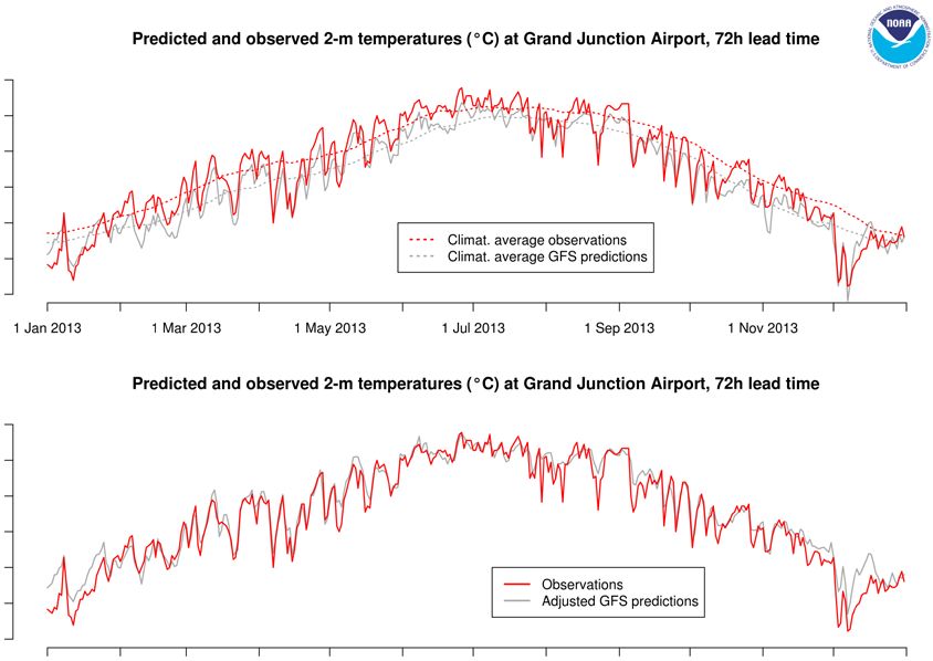
Figure 2 presents a brief example illustrating the potential benefits of statistical postprocessing.
In this example, past numerical forecasts at a certain lead time and the corresponding
observations are available for a certain time period in the past. The upper panel shows the
temporal evolution of the forecasts generated via the Global Forecast System (GFS) without
correction. A clear overall bias is present in the forecasts (estimated from the differences in the
dashed lines). Statistical postprocessing aims to adjust the forecast to remove the estimated bias.
The lower panel shows the forecasts with corrections based on the classical MOS approach of
Glahn and Lowry (1972). This approach will be introduced in Section 3.2.
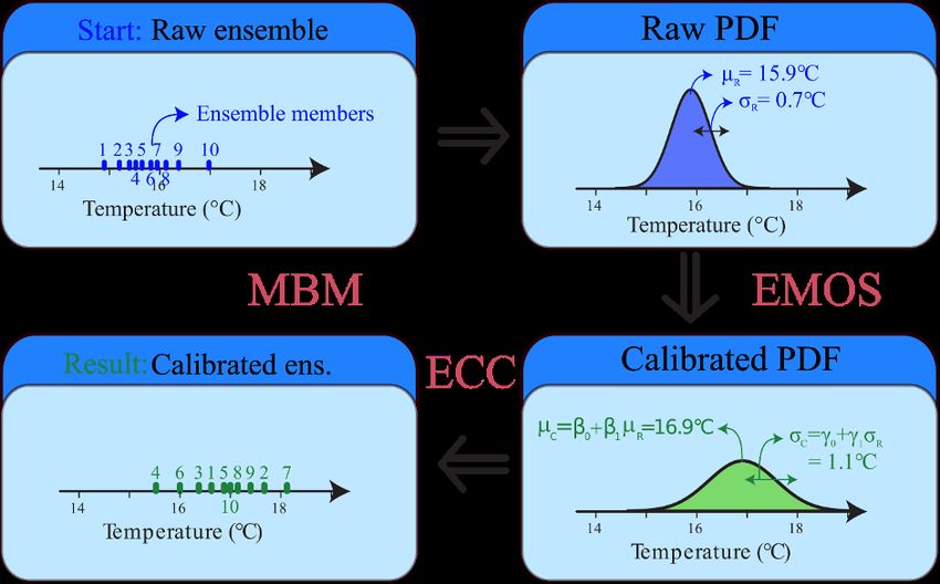
Slightly more complicated corrections can be made to ensemble forecasts to incorporate
corrections for typical overconfidence in raw ensemble forecasts. These corrections fit a
probability density function (PDF) using equations to predict a postprocessed mean and spread
(standard deviation of the ensemble with respect to its mean). This is illustrated in Figure 3. The
40
30
20
10
0
–10 Climat. average observations
Climat. average GFS predictions
–20
Temperature (°C)
1 Jan 2013 1 Mar 2013 1 May 2013 1 Jul 2013 1 Sep 2013 1 Nov 2013
40
30
20
10
0
–10 Observations
Adjusted GFS predictions
–20
1 Jan 2013 1 Mar 2013 1 May 2013 1 Jul 2013 1 Sep 2013 1 Nov 2013
Figure 2. Temporal evolution of predicted (grey) and observed (red) 2-m temperature at
Grand Junction Airport (Colorado, United States of America) at +72 h forecast lead time.
Upper panel: raw forecast; lower panel: postprocessed forecast. The dashed lines in the
upper panel provide smoothed time series to more clearly illustrate the bias.
Source: M. Scheuerer, NOAA/Office of Oceanic and Atmospheric Research/Physical Sciences Laboratory and University
of Colorado/Cooperative Institute for Research in Environmental SciencesCHAPTER 3. UNIVARIATE STATISTICAL POSTPROCESSING 9
40
30
20
10
0
–10 Observations
GEFS predictions
Temperature (°C)
–20
1 Jan 2013 1 Mar 2013 1 May 2013 1 Jul 2013 1 Sep 2013 1 Nov 2013
40
30
20
10
0
–10 Observations
Mean- and spread-adjusted GEFS predictions
–20
1 Jan 2013 1 Mar 2013 1 May 2013 1 Jul 2013 1 Sep 2013 1 Nov 2013
Figure 3. Temporal evolution of predicted (grey) and observed (red) 2-m temperature at
Grand Junction Airport (Colorado, USA) at +72 h forecast lead time. Illustration of an
ensemble MOS approach to statistically adjusting for both bias in the mean forecast and
overconfidence. Top panel: quantiles of the raw ensemble forecast; bottom panel:
statistically adjusted quantiles of the ensemble prediction.
Source: M. Scheuerer, NOAA/Office of Oceanic and Atmospheric Research/Physical Sciences Laboratory and University
of Colorado/Cooperative Institute for Research in Environmental Sciences
grey area in the upper panel represents the spread of values given by the raw ensemble forecast
generated via the Global Ensemble Forecast System (GEFS). If only mean bias is corrected, the
ensemble is overconfident and unreliable. However, the observed temperature, represented
by the red line, frequently lies outside that spread, so the forecast is overconfident in how
accurately it can predict the temperature. The lower panel depicts quantiles of fitted distributions
that account for both corrections to the mean and the spread calculated using ensemble
MOS (EMOS). Popular methods of mean and spread adjustments are presented in Section 3.3.
Different users may desire different types of postprocessed ensemble outputs. Some may simply
want PDFs that are reliable at each observation location or grid point, while others may wish for
the postprocessed guidance to still have realistic variability in time and space. For example, the
raw forecast for ensemble member 1 may be the windiest member at Los Angeles in the western
United States but the least windy member at New York City, and the application (for instance, for
airplane flight routing) may need ensembles with realistic variability in space and time but with
the biases removed. Methods that process the data “univariately”, that is, independently from
one grid point to the next, may destroy the underlying rank-order relationships that existed in
the original ensemble. The focus of this chapter is on univariate statistical postprocessing, but if
the end products are reconstructed ensembles, multiple statistical postprocessing methods may
be possible. Multivariate statistical postprocessing will be addressed in Chapter 4.
The remainder of this section presents an overview of several common univariate techniques,
starting with simple techniques and progressing to more algorithmically complex ones.10 GUIDELINES ON ENSEMBLE PREDICTION SYSTEM POSTPROCESSING
3.1 Deterministic bias correction (Tier 1)
Deterministic bias correction may be suitable for correcting a single-member (deterministic)
forecast or adjusting the mean of an ensemble. It is most suited to variables that have Gaussian
or near-Gaussian distributions and variables whose systematic errors are relatively large
compared to the random errors in the training sample. This method has been used successfully
to adjust many forecast variables such as surface temperature, pressure, and winds. Because of
its simplicity, this method has been applied widely around weather forecast centres and private
sectors for forecast calibration. The Kalman filter-type method (Kalman, 1960), a very simple
method of deterministic bias correction, is described below.
1) Produce a bias-corrected forecast: The bias-corrected forecast Fc(t) on a particular day
of year t and for a given location and forecast lead time is generated by applying a bias
estimate B(t) to the current (raw) forecast F(t). These forecasts are computed independently
for each lead time and each grid point or station location. When the procedure is initiated,
the bias estimate is typically cold-started with a value of 0.0:
Fc ( t )� = � F (� t ) − � B ( t ) 3.1
2) Compute the most recent forecast bias: When the verifying observation becomes
available, the sample forecast bias b(t) is calculated:
b ( t )� = � F (� t ) − � O ( t ) 3.2
3) Update the bias estimate: The running bias estimate is updated using a weighted
combination of the previous day’s bias estimate B(t) and the current day’s sample bias b(t)
using a weight coefficient w:
B ( t + 1)� = � (1 − w
� ) B ( t )� +� � wb ( t ) 3.3
An advantage of the Kalman filter-type bias correction method is that it is easy to implement. The
system does not need to store or save a long time series of prior forecasts; it only needs to update
and save the previous day’s estimate B (t + 1).
The weight w is the parameter that controls the characteristics of the accumulated bias B(t). An
optimal w can be obtained through trial and error. The larger the w, the more the bias estimate
reflects the most recent data, which is appropriate if the bias is quite consistent from day to day
but exhibits some seasonal dependence. A smaller w correspondingly provides greater weight to
samples in the more distant past and is more appropriate if larger samples are needed to quantify
the bias and/or the bias is less seasonally dependent. Practically, the optimal w may be some
function of the forecast variable, forecast lead time, location or seasonality. Many operational
centres use w=0.02 globally for all forecast variables and for all lead times (Cui et al., 2012). When
w=0.02, it estimates the bias with the most recent 50–80 days of information (Figure 4). The
relative impact of older training samples for other decaying average weights such as 0.01 and
0.05 is also shown in Figure 4. The x-axis is for past days (negative number), and the y-axis is for
normalized weight.
An example of the benefit of this simple Kalman filter-type bias correction is shown for northern
hemisphere 2-m temperature using a decaying average weight w=0.02 (Figure 5). Verification
statistics were calculated over the two-month period ending 27 April 2007 and indicate that
mean absolute errors (Wilks, 2019) were reduced by nearly 50% across all lead times.
Like any method, this particular deterministic bias correction has advantages and disadvantages.
Its simplicity is a major advantage, as is the lack of any need to store long training data sets.
A simple method like this, however, may not provide the magnitude of improvement that is
possible with more involved methods, and this method is not applicable for very long training
data sets such as multi-decadal reforecasts. It is also not the method that should be used for
non-Gaussian-distributed variables such as precipitation amount.CHAPTER 3. UNIVARIATE STATISTICAL POSTPROCESSING 11
0.045
w = 0.01
0.040
w = 0.02
w = 0.05
0.035
Normalized values
0.030
0.025
0.020
0.015
0.010
0.005
–200 –180 –160 –140 –120 –100 –80 –60 –40 –20 0
Days
Figure 4. Historical (prior) information (days) used for different decaying average weights
(0.01, 0.02 and 0.05). The decaying average weight is shown as a normalized value. The
accumulated area (under the curve) for w=0.01, w=0.02 and w=0.05 is equal to 19.
Source: Cui et al., 2012
1.0
0.9 gfs_raw
gfs_debias
0.8
Mean absolute error (°C)
0.7
0.6
0.5
0.4
0.3
0.2
0.1
0 0 24 48 72 96 120 144 168
Forecast hours
Figure 5. The average absolute error of northern hemisphere 2-m temperature with forecast
lead times out to 168 hours (7 days) for the period of 28 February 2007–27 April 2007.
National Centers for Environmental Prediction (NCEP) Global Forecast System (GFS) raw
forecast errors (gfs_raw) are in black, and bias-corrected forecast errors (gfs_debias)
are in red.
Source: Yuejian Zhu, NOAA/Environmental Modeling Center12 GUIDELINES ON ENSEMBLE PREDICTION SYSTEM POSTPROCESSING
3.2 Deterministic model output statistics method (Tier 1)
A step up in terms of algorithmic complexity (with respect to the deterministic bias correction
method) involves applying regression analysis procedures that permit corrections not only
for overall biases but also for some state dependence (for example, different biases for warm
versus cold forecast temperatures). The classical MOS correction approach operates on a
single deterministic dynamical forecast available at a specific lead time t, applying multiple
linear regression:
N
Fc ( t ) = α + ∑ βi Fi (t ) 3.4
i =1
Fc(t) is the corrected forecast and Fi(t) is the set of predictors generated by the dynamical model
at time t. The parameters α and βi for i=1, …, N, are estimated by minimizing a cost function,
typically the squared difference between past observations and forecasts coming from a training
sample, which must be archived in contrast to the decaying average bias correction discussed
previously. Often, one of the predictor variables corresponds to the quantity F of interest if it is
available as a prognostic variable in the dynamical model.
The forecast performance of the first raw dynamical model outputs was not as high as those of
the present day, and the MOS equations sometimes included 10 or more additional predictors
(Glahn, 2014), including other dynamical prognostic variables, recent surface observations,
climatological values, and some aspects of seasonality or orography (see, for example,
Jacks et al., 1990). With improved model performance in recent years, fewer predictors
may be needed.
A word of caution about correcting each ensemble member separately
Deterministic forecast errors consist of two components: systematic errors (such as model bias)
and random errors. Ensemble forecasts are designed to account for random errors by sampling the
synoptically dependent uncertainty in the evolution of weather systems, so the ensemble spread
typically increases with increasing forecast lead time. Deterministic forecast corrections such
as those described by Equations 3.1 to 3.4 are designed to correct for systematic errors, but the
data used to optimize the forecasts also include random errors, which increase with forecast lead
time. In applying a MOS procedure to each member of an ensemble with the usual least-square
minimization approach to compute regression parameters, minimizing the effect of the random
errors results in a “regression to the mean” effect, where forecast corrections adjust each member
forecast towards the climatological mean. If such a technique is applied independently to all
members of an ensemble, the regression-corrected ensemble members will exhibit a much smaller
spread, counteracting the ability of the ensemble to represent random errors.
There are several options to counter this effect and retain the spread in the EPS forecast, including:
(i) Using the perfect-prog approach, where the regression corrections are calculated only at
short lead times, when random errors are small, and then applying the same corrections at
all forecast lead times. This approach will correct for consistent model biases and errors in
representation of local conditions by the model while retaining the ensemble spread but will
not correct for any model bias which varies with lead time.
(ii) Using the calculated biases to adjust the ensemble mean forecast at all lead times but then
adding the anomalies from the mean of each ensemble member to the corrected ensemble
mean, thus retaining the ensemble spread. This approach preserves the original ensemble
spread but does not increase it. Increasing the spread is often warranted, however, as raw
ensembles are often under-spread, even after correcting for bias.
(iii) Modifying the cost function of the minimization problem, as is done in Vannitsem (2009)
and Van Schaeybroeck and Vannitsem (2015), in which constraints are imposed to correct
the spread of the ensemble together with its mean. This approach can still be applied to the
individual members and provides reliable ensemble forecasts at all lead times.
Alternative methods which calibrate the entire ensemble distribution rather than treating ensemble
members individually are outlined in following sections.CHAPTER 3. UNIVARIATE STATISTICAL POSTPROCESSING 13
Probabilistic forecasts can also be constructed using Equation 3.4, either by estimating a
predictive distribution – usually Gaussian – around these corrected forecasts (see, for example,
Glahn et al., 2009) or by adjusting each member of an ensemble separately (see, for example,
Van Schaeybroeck and Vannitsem, 2011, 2015). This extension of the MOS concept to ensemble
forecasts allows both the correction of biases due to model errors as well as a representation of
variations in uncertainty based on variations in the ensemble spread.
The classical MOS correction approach, which is based on linear regression, although widely
used and an approach which provides important corrections, is difficult to implement when
dealing with highly non-Gaussian data sets, such as hourly precipitation. This necessitates
the use of alternative approaches. One possibility is to transform the data in order to get an
approximate Gaussian distribution in order to implement classical Gaussian approaches (Hemri
et al., 2015). A second possibility consists of fitting other predictive distributions, such as logistic
or gamma, or even generalized extreme value distributions (see, for example, Wilks, 2018).
Combinations of distributions and truncated distributions are also often used (see, for example,
Baran and Lerch, 2018, for recent applications).
3.3 Ensemble calibration methods
3.3.1 Ensemble model output statistics
(Tier 2 with site observations; Tier 3 on a grid)
Another approach to postprocessing involves adjusting the appropriate probability distributions
for the ensemble of forecasts. This approach is often referred to as ensemble MOS (EMOS)
(Gneiting et al., 2005). One of the most popular EMOS methods is Non-homogeneous Gaussian
Regression (NGR), which consists of fitting a Gaussian distribution to the set of ensemble
members with a mean that is linearly regressed to the observed training data set, as in the
classical MOS method (Equation 3.4), and a variance which depends linearly on the variance
of the ensemble (see Wilks, 2018 for more details). NGR has been shown to work very well for
variables with a probability distribution close to a Gaussian shape, for instance temperature. For
variables such as precipitation or wind, other distributions should be used (see, for example,
Wilks, 2018, Scheuerer and Hamill, 2015) and may be more difficult to implement successfully.
An example demonstrating the application of two postprocessing techniques, a
member-by-member method called Error-in-Variables MOS (EVMOS), introduced in
Vannitsem (2009), and the EMOS-based NGR method, is provided in Figure 6. Both approaches
provide an uncertainty band; however, there is a larger variance for NGR due to the presence
of representativeness errors. Representativeness errors are not accounted for in the EVMOS
method, which only corrects for the impact of model uncertainty at the scale of the model.
In general, the EMOS approach has been used for site forecasts using site observations for
training (Tier 2). However, this approach may also be applied to gridded data using trustworthy
analysis fields in place of observations (Tier 3). This may be done either by calculating the EMOS
coefficients independently at each grid point, by pooling the grid points together to generate a
single set of coefficients for the entire domain or by employing an intermediate approach where
grid points are pooled over a sub-domain. Calculating the EMOS coefficients independently at
each grid point provides optimal local corrections; however, this method requires significant
computational resources in order to generate robust EMOS coefficients and an adequate sample
size within the training data set for each grid point. The method of generating a single set of
EMOS coefficients for the entire domain focuses on correcting a domain-wide bias and will
likely require a reduced training data set (compared to the method of calculating the EMOS
coefficients independently at each grid point), as all grid points within the domain are used in
unison to generate the EMOS coefficients. This method increases the sample size but does not
provide location-dependent error corrections. The intermediate method of pooling grid points
over a sub-domain produces fewer localized corrections than the method which calculates
EMOS coefficients independently for each grid point; however, the corresponding computational14 GUIDELINES ON ENSEMBLE PREDICTION SYSTEM POSTPROCESSING
requirements and training data set requirements are also reduced. One disadvantage of this
method is that there may be discontinuities at the edges of subdomains where biases are
estimated from different samples.
EMOS on the grid Calculation of coefficients Calculation of a single set of coefficients using
at each grid point all grid points
Advantages Local corrections Reduced training data set requirements
to compute robust coefficients
Disadvantages More computationally expensive. Only domain-wide corrections possible
A longer training data set likely
required to compute robust
coefficients.
15
10
5
0
–5
–10
14/02 15/02 16/02 17/02 18/02 19/02
Forecast day
Figure 6. EPS meteograms (EPSgrams) for one specific date (14 February 2009) at Uccle,
Brussels (Belgium). The black dots represent the observation. The ensemble distribution is
represented by the box-and-whiskers, with 50% of the ensemble lying in the inner box and
the remaining members represented by the whiskers. At each lead time, the
box-and-whiskers represent, from left to right, the EVMOS-corrected ensemble (dark grey),
the raw ensemble (light grey) and the NGR-corrected ensemble (dark grey).
Source: Vannitsem and Hagedorn, 2011
3.3.2 Bayesian model averaging (Tier 2)
Another important postprocessing approach involves combining a large set of probability
distributions centred around or associated with a specific ensemble member. The most widely
used method of postprocessing in this manner finds its roots in the Bayesian framework (Raftery
et al., 2005), although it is not fully Bayesian (see Wilks, 2018 for a discussion on this topic). This
method is known as Bayesian model averaging (BMA) and consists of constructing a corrected
probability distribution as
N
( ) ∑wi fi ( Fi ( t ))
f Fc ( t ) = 3.5
i =1
where wi represents the weights given to each distribution f i(Fi(t)) associated with each
ensemble member i=1, …, N. These weights and the distribution parameters are fitted based on a
past training data set. BMA yields a continuous predictive distribution for the forecast variable F.
However, rather than imposing a particular parametric form, BMA predictive distributions are
mixture distributions, or weighted sums of N-component probability distributions, each centredCHAPTER 3. UNIVARIATE STATISTICAL POSTPROCESSING 15
at the corrected value of one of the m ensemble members being postprocessed. This approach
has been used widely for both exchangeable members (where all ensemble members are equally
likely by definition) and non-exchangeable members (see, for example, Sloughter et al., 2010;
Baran, 2014). Other postprocessing methods corresponding to this approach include ensemble
dressing, which was proposed prior to the development of the BMA method (Roulston and
Smith, 2003), and other Bayesian alternatives (see, for example, Marty et al., 2015).
There are disadvantages and reasons to be cautious of the BMA approach. These are discussed in
such publications as Hodyss et al. (2016) and in the references therein.
3.4 Quantile mapping (Tier 2)
For some variables such as precipitation, bias correction may depend on the precipitation
amount and may involve over-forecasts at low precipitation amounts and under-forecasts at
high precipitation amounts. Techniques that are flexible enough to account for state-dependent
biases are thus extremely useful. One approach to addressing state-dependent biases is quantile
regression (Bremnes, 2004), which can also be of much interest when the user does not want to
specify a distribution.
A commonly applied procedure, known as quantile mapping, is illustrated in Figure 7. Quantile
mapping can be applied to a deterministic forecast or individually to members of an ensemble.
In Figure 7, two cumulative probability distributions are represented, one for the forecast and
a second for the observations, which are obtained via a large ensemble of past forecasts. The
red arrows show how the quantile mapping operates: given a forecast of the current day’s
precipitation amount, the quantile associated with this amount is identified, and the forecast
amount is replaced with the observed or analysed amount associated with the same quantile in
the cumulative distribution.
1.0
Non-exceedance probability
0.8
0.6
0.4
0.2
Member forecast
Analyzed
0.0
0 2 4 6 8 10 12 14 16 18 20
Precipitation amount (mm)
Figure 7. Illustration of the deterministic quantile mapping method applied to ensemble
members. Member forecast cumulative distributions and analysed cumulative distributions
are used to adjust the raw forecast value to the analysed value associated with the same
cumulative probability. Red arrows denote the mapping process from forecasts to the
associated quantile determined from training data and back to the analysed quantity
associated with this quantile.
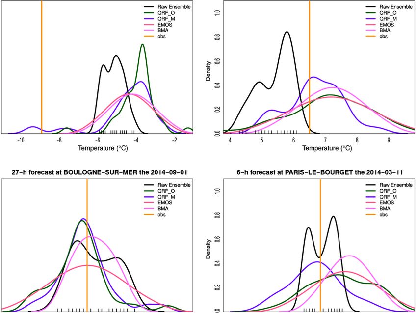
Source: T. Hamill, from Chapter 7 in Vannitsem et al., 201816 GUIDELINES ON ENSEMBLE PREDICTION SYSTEM POSTPROCESSING Quantile mapping is an intuitive and appealing technique in concept. In practice, the differences between the mappings of forecast and analysed/observed distributions may be very large and prone to sampling variability unless large samples are used to generate the underlying cumulative distribution functions (CDFs). In practical applications, data from supplemental locations (other locations with presumed similar forecast characteristics) may be used to populate the CDFs (Hamill et al., 2017), and/or more conservative mapping approximations may be used in the tail of the distribution (Hamill and Scheuerer, 2018) to prevent unrealistically large mappings. 3.5 Machine learning Statistical learning or machine learning methods are used in a wide range of postprocessing approaches in order to extract some key representative features from a set of raw data. These representative features can then be used to infer new outcomes based on new information entering the machine learning algorithm. Machine learning methods are very successful at recognizing patterns in image processing (see, for example, Goodfellow et al., 2016). Deep learning is a particularly effective machine learning method in which the original complex pattern is decomposed into much simpler patterns. Paradigmatic examples are the multi-layer perceptron and the multi-layer neural network that allow the complex link between an input and an output to be decomposed into a multitude of simpler connections between nodes, at which linear or nonlinear functions can transform their own input (see, for example, Goodfellow et al., 2016). This type of method was used quite early in the atmospheric sciences (compared to other fields) for both statistical forecasting (Hsieh and Tang, 1998) and forecast postprocessing (Marzban, 2003; Casaioli et al., 2003) purposes. Early learning approaches used simple forms of neural networks, usually with a single layer between the input and the output. Since then, considerable progress has been made in increasing the types of algorithms (Goodfellow et al., 2016) and also the efficiency of the computing. Simple machine learning techniques, such as employing a single-layer neural network using the standard software routines available in Python libraries, for example, may provide a quick and effective Tier 2-level alternative to some of the statistical techniques, such as MOS, described above. However, care should be taken to ensure that sufficient training data is used to cover a wide range of situations and to keep the neural network simple; otherwise, there is a risk of over-fitting to a small data sample, leading to poor and misleading behaviour with future forecasts. Ensemble learning methods are techniques used for classification and regression based on building decision trees in a training data set. As these are known to be highly dependent on the sample used and prone to over-fitting, randomization is used through bootstrapping and random predictor selection. The result of this randomization is known as a random forest (RF). Once a new realization of predictors is presented to the trees, the split is followed until a leaf is reached. The average situation associated with this leaf from the training sample is the forecast, which is then averaged through all the trees of the random forest. A further development to get distributions instead of the conditional mean has also been proposed and is known as quantile regression forests (QRFs) (Taillardat et al., 2016). An example of the application of the QRF method is displayed in Figure 8. Machine learning techniques will generally be Tier 2 or Tier 3 due to the requirements for managing large quantities of data for training and testing. Whatever machine learning technique is chosen, a key requirement for success is careful attention to the quality control of the data used, which can often be the most time-consuming part of the work. A comparison between neural networks, EMOS and BMA was performed in Rasp and Lerch (2018) and demonstrated the usefulness of adopting machine learning approaches. These approaches can, however, be very demanding in terms of training data.
You can also read