Toward the Personalization of Biceps Fatigue Detection Model for Gym Activity: An Approach to Utilize Wearables' Data from the Crowd
←
→
Page content transcription
If your browser does not render page correctly, please read the page content below
sensors
Article
Toward the Personalization of Biceps Fatigue Detection Model
for Gym Activity: An Approach to Utilize Wearables’ Data from
the Crowd
Mohamed Elshafei                 , Diego Elias Costa       and Emad Shihab *

                                          Department of Computer Science and Software Engineering, Concordia University,
                                          Montreal, QC H3G 1M8, Canada; m_lshafe@encs.concordia.ca (M.E.); diego.costa@concordia.ca (D.E.C.)
                                          * Correspondence: eshihab@cse.concordia.ca

                                          Abstract: Nowadays, wearables-based Human Activity Recognition (HAR) systems represent a
                                          modern, robust, and lightweight solution to monitor athlete performance. However, user data
                                          variability is a problem that may hinder the performance of HAR systems, especially the cross-subject
                                          HAR models. Such a problem may have a lesser effect on the subject-specific model because it is a
                                          tailored model that serves a specific user; hence, data variability is usually low, and performance is
                                          often high. However, such a performance comes with a high cost in data collection and processing
                                          per user. Therefore, in this work, we present a personalized model that achieves higher performance
                                          than the cross-subject model while maintaining a lower data cost than the subject-specific model. Our
                                          personalization approach sources data from the crowd based on similarity scores computed between
                                          the test subject and the individuals in the crowd. Our dataset consists of 3750 concentration curl
                                          repetitions from 25 volunteers with ages and BMI ranging between 20–46 and 24–46, respectively.
                                          We compute 11 hand-crafted features and train 2 personalized AdaBoost models, Decision Tree

                                   (AdaBoost-DT) and Artificial Neural Networks (AdaBoost-ANN), using data from whom the test
Citation: Elshafei, M.; Costa, D.E.;      subject shares similar physical and single traits. Our findings show that the AdaBoost-DT model
Shihab, E. Toward the                     outperforms the cross-subject-DT model by 5.89%, while the AdaBoost-ANN model outperforms
Personalization of Biceps Fatigue         the cross-subject-ANN model by 3.38%. On the other hand, at 50.0% less of the test subject’s data
Detection Model for Gym Activity:         consumption, our AdaBoost-DT model outperforms the subject-specific-DT model by 16%, while
An Approach to Utilize Wearables’         the AdaBoost-ANN model outperforms the subject-specific-ANN model by 10.33%. Yet, the subject-
Data from the Crowd. Sensors 2022,        specific models achieve the best performances at 100% of the test subjects’ data consumption.
22, 1454. https://doi.org/10.3390/
s22041454
                                          Keywords: human activity recognition; wearable sensors; wearable sensor data; machine learning
Academic Editor: Marco Iosa

Received: 21 December 2021
Accepted: 11 February 2022
                                          1. Introduction
Published: 14 February 2022
                                                Fatigue is a natural phenomenon that describes physiological impairments or lack
Publisher’s Note: MDPI stays neutral
                                          of energy caused by prolonged activities [1]. Lately, a plethora of works in the literature
with regard to jurisdictional claims in
                                          about athlete training and monitoring approaches aim to track body performance and
published maps and institutional affil-
                                          measure muscle fatigue for two reasons: (1) fatigue is an important stamina indicator as
iations.
                                          previous studies show that it often occurs prior to muscle injuries in over-training [2–4] and
                                          (2) fatigue-induced injuries are one of the most active research topics in sports science due
                                          to their impact on athletes, such as substantial loss in muscle strength and flexibility [5].
Copyright: © 2022 by the authors.
                                                Often reported as one of the earliest, the invasive approach is used to detect fatigue by
Licensee MDPI, Basel, Switzerland.        measuring the lactic acid in the bloodstream to determine the maximal muscle effort that
This article is an open access article    a person can maintain without risk of injuries [6,7]. Although such an approach requires
distributed under the terms and           puncturing the skin, it often provides accurate information about fatigue conditions and
conditions of the Creative Commons        acetate levels in muscles. A previous study requires several blood samples from athletes
Attribution (CC BY) license (https://     for a blood lactate test to measure their muscle endurance that can provide accurate results
creativecommons.org/licenses/by/          up to 97% [8]. Another previous study that requires blood samples from marathon runners
4.0/).                                    for creatine kinase (CK) tests shows that creatine kinase levels are significantly different

Sensors 2022, 22, 1454. https://doi.org/10.3390/s22041454                                                  https://www.mdpi.com/journal/sensors
Sensors 2022, 22, 1454                                                                                            2 of 24

                         (p-value < 0.05) in muscles during running, which indicates the risk of skeletal muscle
                         injuries [9]. Less painful but respiratory related, the cardio-respiratory approach monitors
                         a person’s fatigue levels by measuring their circulatory and respiratory systems’ ability
                         to supply oxygen to skeletal muscles during sustained physical exercise without risk of
                         injuries [10,11]. Such an approach may require up to five pieces of equipment such as
                         blood pressure cuff, Electrocardiograph (ECG), bicycle, mouthpiece, and saturation monitor.
                         This setup is complex and requires technical expertise to run; hence, it is considered a
                         drawback for daily living applications. However, it accurately estimates the maximum
                         volume of oxygen consumption VO2 during incremental exercises to detect fatigue. A
                         previous study on the oxygen consumption in skeletal muscles measures the respiratory
                         system’s efficiency during sustained physical activity shows that oxygen consumption can
                         provide an accurate indication (>94%) of fatigue intensity [12]. Although the previous
                         approaches may detect signs of fatigue precisely, they often require medical equipment and
                         field training, which makes them too complicated for ordinary users. Recently viewed as
                         the latest, the wearable approach is used to detect fatigue by utilizing sensory data and
                         machine learning algorithms to estimate rates of perceived exertion (RPE) during physical
                         exercises. After the rapid development of low-power wearables, such an approach often
                         represents a modern way to monitor athlete performance and to prevent fatigue-induced
                         injuries during training [13,14]. Previous work on marathon runners that uses data from
                         the inertial measurement unit (IMU) to classify runners as being not-fatigued or fatigued
                         shows that ROC Curves for the General Runners Models, trained using only the statistical
                         features, range between (0.67 and 0.71) [15].
                               HAR applications in motion tracking and athletic training have become more promi-
                         nent as wearable technology and machine learning techniques advance [16,17]. Yet, a
                         common obstacle in such applications is having sufficient data to train the HAR models
                         reliably [18,19]. Training HAR models using insufficient data limits their performance and
                         may even make them impractical for their user base. One way to work around this obstacle
                         is to collect data from a large pool of users and train a cross-subject HAR model. However,
                         this does not guarantee an accurate performance from the cross-subject HAR model be-
                         cause even with sufficient data from a large pool of users, individuals may perform the
                         same activity differently. This increases the inter-subject data variability, which hinders the
                         performance of HAR applications [19]. The inter-subject data variability is often high in
                         places where there is a diverse crowd of users with different physical traits [19,20]. A way
                         to reduce the inter-subject data variability is to address each user separately by collecting
                         data from the user of the HAR application to train a subject-specific HAR model. However,
                         the cost of training a subject-specific HAR model is often prohibitive and requires labeled
                         data from the user [21–23]. Therefore, there is an inherent trade-off between cross-subject
                         models (cheaper but less accurate) versus subject-specific models (more expensive and
                         more accurate). Furthermore, such a trade-off often exacerbates in specialized cases in
                         HAR (e.g., muscle fatigue detection), where manual or semi-supervised labeling is usually
                         required [24,25]. As a result, this increases the data cost in the case of the subject-specific
                         models; or, if we want to spare that data cost, we will choose the less accurate option, the
                         cross-subject models. In this work, we attempt to bridge the trade-off between cross-subject
                         and subject-specific models. We propose a personalization approach that improves the
                         performance of the cross-subject model while utilizing a small sample of the user’s data.
                               To further explain our approach, recent studies show that the personalization of HAR
                         cross-subject models can improve the models’ performance while consuming a part of
                         the test subject’s data less than the subject-specific models [26,27]. The rationale behind
                         the personalization is to prioritize the crowd’s data from whom the test subject is similar.
                         Therefore, we study the physical traits of the crowd to improve personalization of the
                         cross-subject model by adding weights to the training data entries based on the inter-
                         subject similarities between the test subject and the subjects from the crowd [28–32]. We
                         believe that combining similarities measure and personalization can form a personalized
                         model which has a better performance than the cross-subject model and consumes the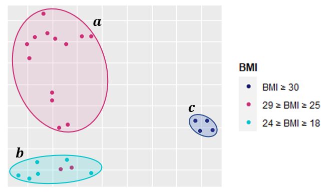
Sensors 2022, 22, 1454 3 of 24
test subject’s data less than the subject-specific models. Moreover, we further enhance the
models’ performance by combining hand-crafted features with some of the suggested ones
from the previous studies [15,33,34]. The hand-crafted features are often specific toward the
activities of interest, which the models have to detect. This further improves the weighting
of the training data based on the similarities between training subjects, the crowd, and the
test subject.
To evaluate our approach, we perform a case study on detecting biceps muscle fatigue
during gym exercise. The study investigates the increasing inter-subject data variability
in data patterns for the same exercise, e.g., bicep curls, among gym-goers due to their
physical properties and movements. Sometimes, introducing a new member to the gym
may increase the inter-subject data variability between the gym-goers if such a member
performs exercises differently from the crowd, wherein this often hinders the HAR models’
performance [35]. A previous study shows that using a subject-specific model to address
each subject may overcome the inter-subject variability challenge, therefore improving the
model’s performance [36]. However, these models are known for their high demand for the
subject’s data which is its major drawback [18]. Moreover, these models often suffer from
dramatic performance drops in real-time applications if the subject’s data are unavailable
or insufficient [37,38].
Detecting bicep muscle fatigue is important because bicep muscle is one of the most
active skeletal muscles in the elbow joint [39,40]. Moreover, bicep fatigue injuries, such
as muscle strain, may require up to 22 weeks of treatment [41,42], while tendon rupture
results in a substantial permanent decrease in flexion and extension strength [43]. This may
delay athletes’ training schedules or their immediate withdrawal from competitions [44].
Therefore, given the detrimental effects of bicep muscle fatigue and the low performance
of cross-subject detection models, we believe that further methods are needed to improve
the performance of the detection models. In our previous work, fatigue detection models
achieved accuracies of 98% and 88% for subject-specific and cross-subject models, respec-
tively. However, we observed that as the inter-subject data variability increases, the gap
between the performance of cross-subject and subject-specific models widens from 10% to
15% [45]. Therefore, in this work, we propose the personalization of cross-subject models
as a solution that provides better performance than cross-subject models while requiring
less data than subject-specific models. Moreover, we provide a set of eleven hand-crafted
features that enhance the performance of personalized fatigue detection models.
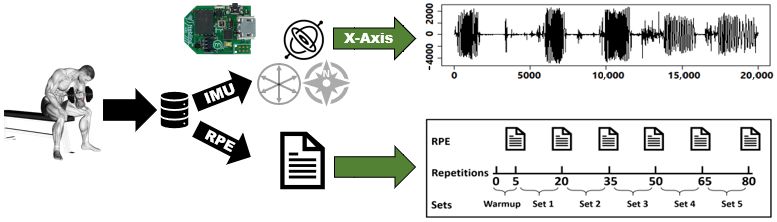
In this work, we employ the personalization of the HAR models to improve the
performance of the bicep fatigue detection models. In Figure 1, we show an overview of
the approach used in this work. First, we select biceps concentration curls as the activity of
interest for this work. Second, we start collecting our data from 25 participants by placing
a 50 Hz Neblina inertial measurement unit (IMU) on their wrist. Meanwhile, on the other
wrist, we place an Apple Watch Series 4 to measure their heart rate during the exercise.
We choose their wrist because it is a primary measuring point for upper limb-related
activities. Third, we manually label each repetition in our dataset as containing fatigue or
not containing fatigue; then, we compute eleven hand-crafted features commonly reported
in the HAR and fatigue-related works. Fourth, we measure two types of similarities,
physical and signal similarities between the test subject and the crowd, and we use these
similarities to add more weight to data collected from individuals in the crowd who are
similar to the test subject. Fifth, we use the weighted dataset to train two machine learning
models: Decision Trees (DT) and Artificial Neural Networks (ANN). Finally, we test these
models using the test subject’s data in detecting fatigue in biceps concentration curls.
Figure 1. Overview of the similarity-based personalization approach for HAR.Sensors 2022, 22, 1454 4 of 24
Our first finding shows that it is preferable for the personalized fatigue detection
models to depend on both physical and signal similarities with a tendency toward signal
similarity. This finding is our first contribution where the eleven hand-crafted features
aid the personalization approach in identifying individuals with similar biceps movement
patterns to contribute more in the training dataset and hence improving the performance
of fatigue detection models. Our second finding shows that the personalization approach
improves the accuracy of the DT model by 5.89% and 3.38% for the ANN model. This
finding is our second contribution where such improvements occur in personalized cross-
subject models after prioritizing training data from the crowd based on the total similarity
score, where individuals with high scores contribute more to the models’ training dataset.
Our third finding shows that we can further improve the accuracy of personalized models
by adding a portion of the test subject’s data to the models’ training datasets. In this
case, the personalized DT model achieves 16.0% higher accuracy than the cross-subject
DT model while consuming 50.0% less of the test subject’s data than the subject-specific
DT model. Moreover, the personalized ANN model achieves 10.33% higher accuracy
than the cross-subject ANN model while consuming 33.33% less of the test subject’s data
than the subject-specific ANN model. This finding is our third contribution where the
personalization approach benefits from the additional data in the training set; yet, it
maintains a comparatively lower test subject data consumption by 33.3% up to 50.0%
compared to the subject-specific models.
The rest of the paper is structured as follows. Section 2 describes how we collect
our dataset and label its entries, as well as illustrates our approach to feature extraction
and measure similarities between the test subject and others from the crowd. In Section 3,
we present our three experiments and research questions; then, we show the results. In
Section 4, we discuss our findings. Section 5 concludes our paper.
2. Materials and Methods
This section describes the details of our dataset and its characteristics to represent a
sample from the crowd. In addition, we demonstrate the processing steps applied to our
dataset to provide a high-quality dataset for our study. Moreover, we extract the eleven
features to detect biceps muscle fatigue. Finally, we describe our approach to measure the
similarity between a test subject and the crowd.
2.1. Dataset Description
We ask twenty-five volunteers to perform concentration curls while we use the fol-
lowing tools to construct our dataset: (1) We attach a 50 Hz Neblina inertial measurement
unit (IMU) to the volunteer’s wrist to measure its acceleration and calculate the linear and
angular velocities. Previous studies show velocity loss as an early indicator of muscle
fatigue during resistance training, especially when blood lactate and ammonia accumulate
in muscle tissues [46–48]. (2) We attach an Apple Watch Series 4 to the volunteer’s opposite
wrist to measure their heart rate during the exercise. (3) We provide the volunteers with a
4.5 kg weight dumbbell to perform concentration curls. (4) We provide the volunteers with
Borg’s scale presented in Table 1 to express their fatigue levels. Such a scale is often used as
a subjective method to estimate the rate of perceived exertion (RPE), which expresses the
fatigue intensity during an exercise. During data collection sessions, we ask each volunteer
to complete 5 warm-up repetitions followed by 15 repetitions per set for a total of 5 sets
per hand, as shown in Figure 2. Moreover, the volunteers report their RPE after each set,
including the warm-up, yielding 6 RPE values per hand.Sensors 2022, 22, 1454 5 of 24
Table 1. Borg G.A. psychophysical bases of perceived exertion [49].
Perceived Exertion Borg Rating Examples
None 6 Reading a book, watching television
Very, very light 7 to 8 Tying shoes
Very light 9 to 10 Chores such as folding clothes that take little effort
Fairly light 11 to 12 Walking through a store (without speeding breath)
Somewhat hard 13 to 14 Brisk walking (mild effort and speeding breath)
Hard 15 to 16 Bicycling, swimming (effort and heart pounding)
Very hard 17 to 18 Intense activity but can be sustained
Very, very hard 19 to 20 Very intense activity that cannot be sustained
Figure 2. Visualization of data acquisition sessions of biceps concentration curl exercise. Rating of
perceived exertion (RPE).
It is essential to explain the rationale behind the tools used in the data collection
sessions, such as the Apple Watch, the 4.5 kg dumbbell, and the Borg’s scale. Borg’s
scale ranges from 6 to 20, where by multiplying these values by ten, we can estimate the
volunteer’s heart rate during the exercise. For example, if a volunteer reports 13 on Borg’s
scale, we should expect to measure their heart rate around 130 to 140 by the Apple Watch.
This serves as a way to strengthen the validity of the reported RPE by each volunteer.
However, in the rare cases of dissimilarity between the Borg scale and the measured heart
rates, we average the reported RPE with the measured heart rate converted to RPE, as
similarly performed in previous work [50]. We use the 4.5 kg weight dumbbell in our
work because of three reasons. The first reason is that several previous works have used
medium-weight dumbbells ranging between 3.5 kg and 5.5 kg to study muscular strength
and fatigue [51–53]. The second reason is that medium-weight dumbbells are often reported
as the most commonly used dumbbells across gym-goers [54]. Third, in previous work,
we found that the 4.5 kg weight dumbbell provides the best trade-off between number
data points recorded in data sessions and time to reach fatigue during an exercise [55].
We use Borg’s scale in our work because we believe that RPE is an appropriate marker
of fatigue as previous studies within sport science have proven that RPE is capable of
modeling a person’s performance better in the real world compared to only heart rate
monitoring [7,49,56].
To aptly evaluate our personalization approach, our dataset should contain sufficient
data from a diverse set of users performing biceps concentration curls for four reasons. First,
with enough data points, we can better capture bicep muscle fatigue, which helps us spot the
variations of fatigue patterns among the volunteers. Second, a diverse dataset strengthens
our work and better represents a sample from the crowd. The twenty-five volunteers are
diverse in age, ranging between 20 and 46, as previous studies show that the selected
age covers three distinct stages of athletes’ performance: early, middle, and late, where
athletes usually notice physical declines [57,58]. Moreover, the twenty-five volunteers
are diverse in weight and height, ranging between 69–127 and 165–190, respectively. ItSensors 2022, 22, 1454 6 of 24
is important to have such variety, as physical characteristics such as weight and height
affect arm movements and the severity of injuries, including fatigue-induced ones [59]. We
calculated the Body Mass Index (BMI) for the twenty-five volunteers using the following
formula [60]:
Weight (kg)
BMI =
Height(m)2
The twenty-five volunteers are also diverse in BMI, ranging between 24 and 46, to
include normal weight (18.5 ≤ BMI ≤ 24.9), overweight (25 ≤ BMI ≤ 29.9), and obesity
(30 < BMI) [61]. The two black dots in Figure 3d are for two volunteers with outlier BMI
values of 41 kg/m2 and 46 kg/m2 who are considered extremely obese [62]. Previous
studies show that the relationship of BMI to injury risk is bimodal, where trainees with
the lowest BMIs exhibit the highest injury risks for both genders and across all fitness
levels [63,64]. In addition, the volunteers have no chronic diseases, no muscle or bone
surgeries, and have been gym-goers for at least 1 year. Moreover, the volunteers are not on
prescribed drugs or substances expected to affect their physical performance.
(a) (b) (c) (d)
Figure 3. Boxplots to display the distribution of volunteers’ age, weight, height, and BMI in
our dataset. (a) Age (years). (b) Weight (kg). (c) Height (cm). (d) BMI (kg/m2 ).
2.2. Dataset Processing
Initially, our dataset contains six signals from the two 3D-accelerometer’s signals (x,
y, z) and the gyroscope. We start by extracting and labeling the repetitions into fatigue
and non-fatigue repetitions. Figure 4 shows an example of the fifth set of repetitions in
its raw data form. In this example, the raw data are extracted from the gyroscope’s x-axis
along with their corresponding RPE values reported by the volunteer. A previous study on
quantifying muscle fatigue suggests an RPE value of 16 as the threshold of true fatigue to
estimate the declines in muscle strength during tasks [65]. Therefore, we extract and label
each repetition manually according to the RPE values reported for the set, where we label
repetitions with reported RPE values larger than 16 as fatigue and others as non-fatigue
repetitions. The figure shows two distinct groups of non-fatigue and fatigue repetitions
extracted from the set. The troughs indicate full extension, while peaks indicate full flexion.
We repeat the same process for the remaining 4 sets.Sensors 2022, 22, 1454 7 of 24
Figure 4. An example of extracting and labeling repetitions of the fifth set from the gyroscope’s
x-axis.
However, the process is not as exhausting as it may seem per volunteer because we use
a synchronized IMU. Therefore, we only need to fully extract and label all 5 sets recorded
by one axis per volunteer, e.g., gyroscope’s x-axis. Then, we use the same timestamps from
the gyroscope’s x-axis to extract and label repetitions for all the remaining signals (other
axes of gyroscope and accelerometer). After we processed all data from the volunteers, our
dataset consisted of 3750 repetitions recorded from 6 time-series signals. We compute three
additional signals, which are total acceleration, exerted force, and acc–gyro data fusion, as
the following:
• Total acceleration: This is the vector sum of the tangential and centripetal accelerations,
which makes it a place-independent signal. Hence, total acceleration does not rely on
the exact attachment of the accelerometer because it combinesqx, y, and z acceleration
signals at time ti to compute a total acceleration, defined as: a2xi + a2yi + a2zi .
• Exerted force: Fexerted = m × a is the exerted force by the volunteer to lift the dumbbell.
Fexerted is calculated by multiplying the mass m of the lifted dumbbell by acceleration
a.
• Acc–gyro data fusion (complementary filter): A complementary filter is often used
to detect human body movement patterns by combining the gyroscope and the ac-
celerometer [66,67]. Gyroscope’s data are used for precision because it is not vul-
nerable to external forces, while the accelerometer’s data are used for long-term
tracking as it does not drift. We use the Kalman filter algorithm to estimate roll,
pitch, and yaw angles [68]. However, we use the yaw angle because it indicates the
sideways vibration for the volunteer’s hand during the extension and flexion of the
bicep. Previous studies show fatigue may cause a temporary movement disorder,
such as skeletal muscles vibration, which indicates fatigue backlogs and increases
the vibration angle [69–72]. In the filter’s simplest form, the equation is defined as:
angle = 0.98 × ( angle + gyro × dt) + 0.02 × acc.
2.3. Feature Extraction
Feature extraction is a crucial component of HAR systems because it establishes the
most significant parameters to identify or predict human body movements. In addition, fea-
ture extraction reduces the data dimensionality while preserving the relevant characteristics
of the signal. In this work, we compute a total of eleven hand-crafted features, as shown
in Table 2. Eight of the selected features are proven accurate in previous works, especially
in the general classification of human activities [15,33,34,73–75]. These features include
min, max, mean, median, SD, variance, kurtosis, and RMS. Besides the eight features
mentioned before, we also select three other features often associated with fatigue for better
performance: skewness, IoP, and MSP [76–79]. A previous study suggests considering
the skewness of the data when detecting fatigue in repetitive muscle movements such as
bicep curls [55]. We select skewness as a fatigue feature because, during the repetitions’
extraction and labeling process, we observed the following: (1) Non-fatigue repetitions
are relatively symmetrical during the repetitions’ extraction and labeling process. (2) InSensors 2022, 22, 1454 8 of 24
contrast, fatigue repetitions are often positively skewed. Another work shows that fatigue
often occurs in later sets, which increases the time to complete repetitions of bicep curls
while decreasing the force exerted by the muscles [45]. This is observable through the
increments of intervals between peaks, e.g., IoP, and decrements of peaks’ amplitudes, e.g.,
MSP. For each volunteer, we extract the eleven features on all repetitions, across all nine
signals, including the two 3D signals (x, y, z) from the accelerometer and the gyroscope,
total acceleration, exerted Force, and acc–gyro signal fusion.
Table 2. Eleven hand-crafted features: eight HAR-related features and three fatigue-related features.
Feature Formula
Minimum min = mini=1,...N ( xi )
Maximum max = maxi=1,...N ( xi )
Mean x= 1
N ∑iN=1 xi
(
x N +1 , N odd
Median M= 1
2
Centralized 2 (x N
2
+ x N +1 ), N even
2
q
Standard Deviation (SD) σ= 1
N ∑iN=1 ( xi − x )2
Variance σ2 = 1
n ∑in=1 ( xi − x )2
( x − x )4
Kurtosis K= ∑iN=1 i σ4
1
N
q
Root Mean Square (RMS) RMS = N1 ∑iN=1 ( x− x )2
( x i − x )3
Skewness Sk = 1
N ∑iN=1 σ3
Fatigue Interval of Peaks (IoP) IoP = Tp − Tp−1 : p = 2, ...N
p j − pi
Mean Slope between Peaks (MSP) MSP = 1
N2 ∑iN=1 ∑ N
j =1 Tp j − Tpi
2.4. Extracting Similarities
To visualize the concept of our work, let us assume that a test subject is selected from a
diverse population P of size n, as shown in Figure 5. Each member of the population reports
their physical traits along with bicep concentration curl data signals. Meanwhile, the test
subject provides only partial data, often one set of repetitions, of their bicep concentration
curl data signals along with their physical traits. We measure the similarities between the
test subject and members of the population so that the data from whom the test subject
is similar gain more weight while training the model. We are keen to utilize two types
of similarities, physical similarity and signal similarity, because previous studies have
reported gains in performance when harnessing those similarities to weight data from the
crowd [28,31].
We believe that combining both physical and signal similarities may further improve
the personalized models’ performance. Therefore, in the second research question (RQ2),
we measure and compare the performance between the personalized models trained using
the weighted data and the cross-subject models. Furthermore, it comes to our minds that
if we already possess and use a part of the test subject’s data to measure the similarities
between the test subject and the crowd, then we may let the personalized models consume
it in training to improve their learning. Therefore, in the third research question (RQ3), we
also decided to let subject-specific models consume the same part of the test subject’s data;
then, we compare the performances of personalized and subject-specific models. Moreover,
we allow the subject-specific models to consume more of the test subject’s data if neededSensors 2022, 22, 1454 9 of 24
until it can reach the same performance of personalized models so that we quantify the
amount of spared data by using personalized models.
Figure 5. Visualization of the concept of personalizing general model using crowd-sourced wear-
ables’ data.
2.4.1. Measuring Physical Similarity
Physical characteristics of people (e.g., age, weight, height, or BMI) vary from one
person to another within a large population. Such differences can affect the way people
move and perform physical activities. We believe that a user with different physical traits,
e.g., age and BMI, may show signs of fatigue differently. At the same time, we expect
groups of people who share similar physical traits to show similar signs of fatigue [80,81].
For example, let us capture the signs of fatigue using the three fatigue-related features,
skewness, IoP, and MSP, and plot the principal component analysis (PCA). In Figure 6a,
we often observe that individuals within specific limits of BMI values tend to share similar
signs of fatigue. Moreover, Figure 6b shows similar observations where we use age instead
of BMI. We can observe that individuals of certain ages tend to share similar signs of fatigue.
This strengthens our hypothesis that if we construct the training data from individuals
within the population who are more similar, it may reduce the inter-subject data variability
and hence improve the performance of the fatigue detection model.
(a) (b)
Figure 6. PCA plots showing signs of fatigue captured by the three fatigue-related features and
BMI/age. (a) BMI perspective. (b) Age perspective.
To compute the physical similarity value between a pair of users, we employ four
types of physical traits: age, height, weight, and BMI. To limit the widespread of the values,
due to subjects’ variations, we apply min–max normalization to each physical trait, on
training data, to normalize each trait between 0 and 1. We combine these four traits per user
to form a dedicated physical vector V Phy = {age, height, weight, BMI} representing their
physical traits separately. We measure the distance d Phy between the physical traits V Phy of
two users (q, p) based on the Manhattan distance, as shown in Equation (1). Previous works
show that Manhattan distance is preferable to Euclidean for high dimensional data and if
the dimensions are not comparable [82–84]. The physical similarity between users (q, p)
is based on the universal law of generalization proposed in previous works [28,31,85,86],Sensors 2022, 22, 1454 10 of 24
where distance and perceived similarity are related via an exponential function, as shown
in Equation (2):
4
∑ |Vqk
Phy Phy
d Phy (q, p) = − Vpk | (1)
k =1
1
sim Phy (q, p) = Phy
(2)
eγd (q,p)
where γ is an empirically determined scaling parameter that affects the shape of the
exponential function. For example, limγ→∞ sim Phy (q, p) = 0, which indicates that as γ
approaches infinity, the physical similarity approaches zero, causing more segregation
between users. This can be a double-edged sword because as we segregate dissimilar users
from each other, we may increase the segregation between similar users unintentionally.
On the other hand, limγ→0 sim Phy (q, p) = 1, which indicates that as gamma approaches
zero, the physical similarity approaches one, implying that all subjects show similar signs
of fatigue; in other words, the changes in their data patterns are similar. Again, this is a
double-edged scenario where we may unintentionally pull dissimilar users near to the
similar users. Therefore, further investigation is required to estimate the optimal value
of γ.
2.4.2. Measuring Signal Similarity
In the context of signal similarities, we use one set of repetitions, approximately 20%
of the subject’s data needed for the subject-specific models. We believe that users within
the same population may show similar signs of fatigue, leading to similar changes in data
patterns while performing the exercise. To compute the signal similarity value between
a pair of users, we employ the 11 extracted features in Table 2 to form a dedicated signal
vector V Sig = {min, max, ... , MSP} for each user. We measure the distance dSig between
the signal traits V Sig of two users (q, p) based on the Manhattan distance for all repetitions
l = {1, 2, ... , L}, as shown in Equation (3).
11 L
∑ ∑ |Vq(k,l) − Vp(k,l) |
Sig Sig
dSig (q, p) = (3)
k =1 l =1
1
simSig (q, p) = Sig
(4)
eγd (q,p)
The signal similarity between users (q, p) is based on the distance between their
vectors, as shown in Equation (4).
2.4.3. Measuring Total Similarity
We measure the total similarity sim Total between two users (q, p) by summing their
weighted physical sim Phy (q, p) and signal simSig (q, p) similarities, as shown in Equation (5).
sim Total (q, p) = α × sim Phy (q, p) + β × simSig (q, p) (5)
where α + β = 1. If α is greater than β, the physical similarity will contribute more than
signal similarity in determining the total similarity value. On the other hand, if β is
greater than α, the signal similarity will be the one that dominates the total similarity value.
Therefore, in the first research question (RQ1), we further investigate the impact of (α, β)
values on the performance of the personalized models. Moreover, we examine (γ) values
to achieve the highest performance possible.
3. Experiments and Results
In this section, we describe the setup to evaluate the personalization approach in
boosting the performance of cross-subject models. We start by listing the three researchSensors 2022, 22, 1454 11 of 24
questions and the selected models for the experiment setup. Then, we identify the possible
values for the parameters (α, β, γ) in Equations (2), (4), and (5).
• RQ1: What is the impact of the physical and signal parameters on the performance of
the personalized biceps fatigue detection models?
• RQ2: Can the personalization approach improve the performance of cross-subject
models in detecting biceps muscle fatigue?
• RQ3: Can the personalization approach reduce the consumption of the test subject’s
data in comparison to subject-specific models?
We employ two models that utilize weighted data in the training to improve classifi-
cation performance. Several works in the literature suggest using AdaBoost, a statistical
boosting technique used as an ensemble method to reduce error in generalized models
at the cost of weighing the training data [87–89]. Therefore, we use AdaBoost to take
advantage of weighting the data, as mentioned in Section 2.4, while training these models.
We select two models that have been previously used in HAR-related applications. The
first model is the Decision Tree (DT); this model was used to count and classify ambulatory
activities using eight plantar pressure sensors within smart shoes in a previous study [90].
The second model is the Artificial Neural Networks (ANN); this model was used to detect
and count repetitions for complex physical exercises [91]. Specifically, we use Adaboost-
backpropagation neural network, which is used in HAR-related works [92,93]. There are
two reasons for choosing DT and ANN among several other machine learning algorithms.
(1) The current work aims to mitigate the hindering effect of subject data variability on
cross-subject models, which we previously encountered in our prior work [45]. Therefore,
we used the same models as in our previous work to fairly examine whether our person-
alization approach can minimize such a problem. (2) We wanted to examine a previous
study finding that AdaBoost often achieves higher improvement on weak classifiers such
as DT than stronger ones such as ANN [92].
In this work, we construct the training dataset based on the similarity score between
the test subject and the crowd. The data from whom the test subject has the highest
similarity score are used in validation/ tuning the models, while the remaining data are
used to train the models. On the other hand, the test dataset is unseen data collected from
the test subject and used only to assess the performance of the models.
3.1. Examining the Hyper-Parameters in the Personalized Biceps Fatigue Detection Model
In this section, we state our motivation and approach for RQ1. Our motivation for RQ1
is that we believe the performance of users similarity-based models, such as those driven
from the personalization approach, may degrade if the inadequate parameters are selected.
In other words, valuable data from the crowd, e.g., similar users, may be discarded due to
an unintended preference for the physical similarity over signal similarity and vice versa.
Previous work shows that finding a balance between the extracted similarities is important
to improve the accuracy of the models constantly [94].
Our approach to address RQ1 is that we examine the possible values for the parameters
(α, β, γ) in Equations (2), (4) and (5) so that we observe the impact of these parameters on
the models’ performance. We start with Equations (2) and (4) to examine γ, which has
an arbitrary value between (0, ∞). To observe the impact of the different γ values on the
models’ performance, we employ each γ value to run two pairs of models: AdaBoost-DT
and AdaBoost-ANN. The first pair is physical similarity-based models of AdaBoost-DT and
AdaBoost-ANN, while the second pair is signal similarity-based models of AdaBoost-DT
and AdaBoost-ANN. Then, we compute the changes in these models’ performance as the
value of γ increases and select the gamma value that corresponds to the best performance.
In Equation (5), we examine the physical α and signal β parameters while satisfying the
condition α + β = 1. We experiment with different α and β values and observe the effect by
running two similarity-based models (AdaBoost-DT, AdaBoost-ANN). Then, we compute
the models’ performance as the values of α and β change; then, we select the (α, β) values
that correspond to the best performance.Sensors 2022, 22, 1454 12 of 24
3.1.1. RQ1: What Is the Impact of the Physical and Signal Parameters on the Performance
of the Personalized Biceps Fatigue Detection Models?
Figure 7 shows the average changes in both models’ performance as the value of γ
increases. The performance in this context is measured using accuracy. We use the accuracy
at γ = 0 as the reference point to measure the changes in accuracy (∆Accuracy) as the γ
value increases. We observe that ∆Accuracy increases as the γ value increases until both
reach maximum values of 3.83 and 14 at the dashed line, respectively. Then, the changes
in accuracy start to decline as the γ value continues to increase. Therefore, we select the
γ = 14 to let the models perform at maximum accuracy.
Figure 7. The average changes in both models’ accuracy as the value of γ increases.
Figure 8 shows the impact of the physical α and signal β parameters on models’
performance and there are three important findings in the figure. In the first finding, at
α = 0 and β = 1, the models (AdaBoost-ANN, AdaBoost-DT) solely depend on the signal
similarity, leading the training dataset, for these models, to be selected from the crowd with
whom the test subject’s signal is similar while discarding the physical similarity. In this case,
the two models (AdaBoost-ANN, AdaBoost-DT) achieve accuracy of 82.13% and 62.49%,
respectively. In the second finding, at α = 1 and β = 0, the models (AdaBoost-ANN,
AdaBoost-DT) solely depend on the physical similarity, leading the training dataset, for
these models, to be selected from the crowd with whom the test subject’s physical traits is
similar while discarding the signal similarity. In this case, the accuracy for the two models
(AdaBoost-ANN, AdaBoost-DT) drops to 81.07% and 62.52%, respectively. In the third
finding, at α = [0.25, 0.50] and β = (1 − α), the models (AdaBoost-ANN, AdaBoost-DT)
depend on both physical and signal similarities; however, the training dataset, for these
models, is selected from the crowd with whom the test subject’s is similar while prioritizing
those with the highest signal similarity. In this case, we observe that the accuracy for the
two models (AdaBoost-ANN, AdaBoost-DT) rises to reach 84.54% and 65.88%, respectively.Sensors 2022, 22, 1454 13 of 24
Figure 8. The average models’ accuracy as the values of α and β change.
3.1.2. RQ1 Conclusion
Our findings show that both physical and signal similarities are important. Moreover,
the models’ performance reaches its peak when γ = 14. The best selected values for α = 0.4
and β = 0.6 which we use for the rest of the evaluations.
3.2. Evaluating the Performance of Personalized Models
In this section, we state our motivation and approach for RQ2. Our motivation for RQ2
is that cross-subject models may seem preferable when it comes to a large number of users.
However, a common trade-off for having cross-subject models is accuracy loss, especially
for users with particular activity patterns. In other words, users who do not share enough
similarities with the crowd may look as outliers where the cross-subject models are less
accurate to detect their biceps muscle fatigue. We believe that adding weight to user’s data
from whom the test subject is similar can improve model accuracy, including marginal
users. Results of a previous study show that the personalization of cross-subject models
constantly improves their accuracy compared with the standard cross-subject models [27].
True( Fatigue + NonFatigue)
Accuracy = (6)
True( Fatigue + NonFatigue) + False( Fatigue + NonFatigue)
True( Fatigue)
Precision = (7)
True( Fatigue) + False( Fatigue)
True( Fatigue)
Recall = (8)
True( Fatigue) + False( NonFatigue)
2 ∗ Precision ∗ Recall
F1 = (9)
Precision + Recall
Our approach to address RQ2 is that we use the 11 hand-crafted features along with
the 2 similarity-based models (AdaBoost-DT, AdaBoost-ANN). We use these models to
predict the Borg rating for each repetition, detecting whether a repetition contains fatigue or
not. We run two experiments. In the first experiment, we set (α = 0, β = 0) in both models
to mimic the standard cross-subject models. This means that the training dataset for theseSensors 2022, 22, 1454 14 of 24
models is collected without considering any type of similarity between the crowd and the
test subject. For this experiment, we use leave-one-out cross-validation (LOOCV), which
is a K-fold cross-validation with K equal to the number of volunteers (K = 25). In the
second experiment, we set (α, β) to optimal values as identified in Section 3.1.1, leading the
training dataset, for these models, to be selected based on physical and signal similarities,
in addition to prioritizing data coming from users of highest signal similarity in the crowd.
For each experiment, we calculate the accuracy using the confusion matrix shown in
Table 3, where non-fatigue repetition represents a Borg score from 6 to 16, and fatigue
status represents a Borg score from 17 to 20. We calculate the accuracy using Equation (6),
precision using Equation (7), recall using Equation (8), and F1 using Equation (9).
Table 3. Fatigue detection confusion matrix.
Actual
Fatigue ∈ [17,20] Non-Fatigue ∈ [6,16]
Fatigue ∈ [17,20] TRUE Fatigue FALSE Fatigue
Predict
Non-Fatigue ∈ [6,16] FALSE Non-Fatigue TRUE Non-Fatigue
3.2.1. RQ2: Can the Personalization Approach Improve the Performance of Cross-Subject
Models in Detecting Biceps Muscle Fatigue?
It is important to mention that we use one set of 15 repetitions approximately from the
test subject’s data during the personalization of DT and ANN to measure the signal similar-
ity between the test subject and individuals in the crowd. However, we do not include these
15 repetitions nor any data from the test subject in the training set. Our findings show that
the personalization approach improves the accuracies for the models by 5.89% (DT) and
by 3.38% (ANN), as shown in Table 4. The accuracy improved after prioritizing training
data from the crowd based on the total similarity score, where individuals with high scores
contribute more to the models’ training dataset. Moreover, we observe other improvements
in terms of precision, recall, and F1-measure across the models. The results show that
the personalization improves the DT model in terms of precision by (1.20%), recall by
(4.51%), and F1-measure to (2.81%). On the other hand, the personalization improves the
ANN model in terms of precision by (6.96%), recall by (4.55%), and F1-measure to (5.82%).
Moreover, we observe that the standard cross-subject ANN model outperforms both DT
models, which is expected in fatigue detection wherein ANN models often perform better
than other cross-subject models [95].
Table 4. Average precision, recall, and accuracy, with a CI of 95%, for detecting fatigue in biceps
repetitions before and after the personalization of cross-subject models.
Models
DT ANN
Cross-Subject Personalized ∆ Cross-Subject Personalized ∆
Precision 60.57% ± 0.66 61.77% ± 0.58 1.20% 73.29% ± 0.43 80.25% ± 0.47 6.96%
Recall 61.32% ± 0.53 65.83% ± 0.49 4.51% 78.53% ± 0.39 83.08% ± 0.43 4.55%
Accuracy 60.08% ± 0.49 65.97% ± 0.67 5.89% 82.41% ± 0.58 85.79% ± 0.48 3.38%
F1 60.94% ± 0.59 63.75% ± 0.53 2.81% 75.82% ± 0.41 81.64% ± 0.45 5.82%
3.2.2. RQ2 Conclusion
Overall, our findings indicate that the personalization approach improves both models
in terms of performance. For the DT model, the personalization improves its F1-measure
from (60.94%) to (63.75%), while for the ANN model, the personalization improves its F1-
measure from (75.82%) to (81.64%).Sensors 2022, 22, 1454 15 of 24
3.3. Examining the Consumption of the Test Subject’s Data in the Personalization Approach
In this section, we state our motivation and approach for RQ3. Our motivation for RQ3
is that subject-specific models are known for their high performance and demand of the test
subject data. On the other hand, the cross-subject models are known for their relatively lower
performance and no test subject data demand. We believe that the personalized approach can
combine the best aspects of these two models. In other words, the personalization approach
can improve the performance of the cross-subject models while consuming less test subject
data than the subject-specific models. A previous work shows that adding a small amount of
the test subject’s data to the training dataset for personalized models helps to improve the
performance further closer to the subject-specific models [36].
Our approach to address RQ3 is that we utilized the 11 hand-crafted features and
4 models: subject-specific (DT, ANN) models and personalization (AdaBoost-DT, AdaBoost-
ANN) models. We use these models to predict the Borg rating for each repetition to
determine whether it is fatigue repetition or not. Similar to RQ2, we set (α, β) to optimal
values so that the training dataset for these models is selected based on physical and signal
similarities while prioritizing the signal similarity selection. Our experiment consists of
seven runs where we incrementally add 10% of the test subject’s data to the training set after
each run. This means, there is 0% of the test subject’s data added to the training dataset at
the 1st run, while at the 7th run, there is 60% of the test subject’s data added to the training
dataset. We stop at 60% of the test subject’s data to prevent overfitting the personalized
model; otherwise, there will not be much of a difference between the subject-specific and
the personalization approaches. Moreover, this allows us to measure the amount of the test
subject’s data needed to improve the personalization models’ performance closer to the
subject-specific models. Or, in other words, how little data we need from the test subject if
we use the personalized models instead of subject-specific ones while keeping the accuracy
relativity high. For each run, we calculate the accuracy using Equation (6) and accuracy
gain ratio (AGR) using Equation (10).
∆accuracy
AGR = (10)
Test subject’s data (repetitions)
3.3.1. RQ3 Results: Can the Personalization Approach Reduce the Consumption of the Test
Subject’s Data?
Our findings show that the more the test subject’s data are added to the training set,
the higher the accuracy of the subject-specific and personalized models. Table 5 shows that
the subject-specific DT model achieves an accuracy of 78.90% after consuming 40% of the
test subject’s data. On the other hand, the personalization of the DT model achieves an
accuracy of 76.08% after consuming 20% of the test subject’s data while compensating the
rest of the training data from the similar users in the crowd. In other words, the subject-
specific DT model requires twice the amount of test subject data, at 40%, to achieve similar
accuracy to the personalized DT at 20% of the test subject’s data consumption with taking
into consideration that the personalized DT model compensates the rest of the training data
from the crowd. Moreover, our findings show that with 20% of the test subject’s data, the
personalized DT model reaches the lowest accuracy gain ratio of 0.36% per test subject’s
repetition while maintaining the highest accuracy gain of 5.44%.
Furthermore, the subject-specific ANN model achieves an accuracy of 92.99% after
consuming 60% of the test subject’s data. On the other hand, the personalization of the
ANN model achieves an accuracy of 92.74% after consuming 20% of the test subject’s data
while compensating the rest of the training data from the similar users in the crowd. In
other words, the subject-specific ANN model requires triple the amount of test subject’s
data, at 60%, to achieve similar accuracy to the personalized ANN at 20% of the test
subject’s data consumption with taking into consideration that the personalized ANN
model compensates the rest of the training data from the crowd. Moreover, our findings
show that with 20% of the test subject’s data, the personalized ANN model reaches theSensors 2022, 22, 1454 16 of 24
lowest accuracy gain ratio of ≈0.36% per test subject’s repetition while maintaining the
highest accuracy gain of 5.37%.
Table 5. The accuracy averages for the subject-specific and personalized models after adding 10% of
the test subject’s data to the training set in each run incrementally. We include a version of this table
with the confidence intervals in the Appendix A.
Number of Biceps Repetitions Collected from the Test Sub-
ject (% of Used Test’s Data)
0 8 15 23 30 38 45
(0%) (10%) (20%) (30%) (40%) (50%) (60%)
Accuracy 15.34% 41.30% 58.40% 68.60% 78.90% 82.20% 84.03%
Subject-specific ∆accuracy - 25.96% 17.10% 10.20% 10.30% 3.30% 1.83%
AGR - 3.25% 1.14% 0.44% 0.34% 0.09% 0.04%
DT Accuracy 65.88% 70.64% 76.08% 77.77% 79.15% 79.55% 79.91%
Personalized ∆accuracy - 4.76% 5.44% 1.69% 1.38% 0.40% 0.36%
Models AGR - 0.60% 0.36% 0.07% 0.05% 0.01% 0.01%
Accuracy 55.23% 62.48% 74.68% 82.95% 87.37% 90.45% 92.99%
Subject-specific ∆accuracy - 7.25% 12.20% 8.27% 4.42% 3.08% 2.54%
AGR - 0.91% 0.81% 0.36% 0.15% 0.08% 0.06%
ANN Accuracy 84.54% 87.37% 92.74% 93.56% 93.88% 94.25% 94.78%
Personalized ∆accuracy - 2.83% 5.37% 0.82% 0.32% 0.37% 0.53%
AGR - 0.35% 0.36% 0.04% 0.01% 0.01% 0.01%
3.3.2. RQ3 Conclusion
Our findings show that the personalization approach may reduce the test subject’s
data consumption by 33.3% up to 50.0% while reducing the accuracy gap compared to the
subject-specific models.
4. Discussion
This section discusses our findings, points out work limitations, and proposes future works.
4.1. Findings Discussion
In RQ1, we observe that ∆Accuracy increases following a γ increase until it reaches a
maximum of 3.83 at γ = 14. Then, the accuracy starts to drop slightly with higher values
of γ. Previous studies report similar behavior for the gamma parameter in their results
sections [28,31]. They observe their models’ accuracy increases with an increase in γ value
until γ reaches an optimal point, where their models then start losing accuracy. Although
gamma’s behavior seems similar, the γ values are different and depend on the dataset.
The reason behind gamma’s behavior resides in Equations (2) and (4) where we find that
the physical and signal similarities approach zero as γ → ∞. This means, if we keep
increasing the gamma values, we will push the test subject further away from the crowd.
In other words, we, unintentionally, decrease the possibility of finding similar users in the
crowds, resulting in fewer similar data points, and hence smaller training data. On the
other hand, when γ → 0, the physical and signal similarities approach 1. This means, if we
keep decreasing the gamma values, we will push the test subject closer toward the crowd,
increasing the possibility of finding similar users. However, this can increase the risk of
including low-quality data points from similar users with low ranks, which is usually the
case in a cross-subject model; therefore, the accuracy often drops.
In RQ2, our findings show improvements in accuracy for both personalized models,
AdaBoost-DT and AdaBoost-ANN, compared to the standard cross-subject ones, by 5.89%
and 3.38%, respectively. Such improvements occur because the training datasets for the per-
sonalized models are selected from users who’s physical and signal traits are similar to the
test subject. A previous study reports similar findings to ours, indicating that personalizedSensors 2022, 22, 1454 17 of 24
models often perform +3% better than standard cross-subject models [27]. However, their
proposed personalized model averages 0.78 for F1-score, while our AdaBoost-ANN model
performs 3.64% better with an average of 81.64% ± 0.45 for F1-score. Overall, while this
has been shown in previous works, our results help consolidate the benefits on relying on
similarity as a method for boosting the performance of cross-subject models.
In RQ3, our finding indicates that the personalized models, AdaBoost-DT and AdaBoost-
ANN, achieve comparable performance to subject-specific models while consuming 50.0%
and 66.77% less test subject data. This is an important finding to motivate approaches that
rely less on the data of the subject, particularly in cases where the test subject’s data are
difficult to obtain or very limited. A previous study utilized a personalization approach to
cut down the cost of data labeling by up to 90% for new users [37]. The study reports model
accuracy between 77.7% and 83.4%. In contrast, we can observe that our personalized models,
AdaBoost-DT and AdaBoost-ANN, achieve closer or higher accuracies at 76.08% ± 0.71
and 92.74% ± 0.49 at similar rates of 20% test data consumption, respectively, as shown
in Table 6. This table shows the accuracy achieved by fatigue detection models including
the cross-subject, subject-specific, and personalized models. As an implication, our findings
suggest that personalized models are an effective approach to reduce data dependency—when
data on the target subject is scarce—without severely compromising the model’s performance.
Table 6. Percent accuracy achieved on, with a CI of 95%, the cross-subject, subject-specific, and
personalization models.
∆Accuracy
(% of Used Test’s Data) Accuracy
Cross-Subject Personalized Subject-Specific
Cross-Subject (0%) 60.08% ± 0.49 - −16.00% −28.67%
DT Personalized (20%) 76.08% ± 0.71 16.00% - −12.67%
Subject-Specific (100%) 88.75% ± 0.59 28.67% 12.67% -
Models
Cross-Subject (0%) 82.41% ± 0.58 - −10.33% -16.89%
ANN Personalized (20%) 92.74% ± 0.49 10.33% - −6.56%
Subject-Specific (100%) 99.30% ± 0.37 16.89% 6.56% -
Moreover, we can observe that both of the personalization models achieve higher
accuracies compared to the cross-subject models. However, we find that the personal-
ization ANN models achieve lesser accuracy improvement than the personalization DT
models. This agrees with previous work that shows that AdaBoost usually achieves higher
improvement results on weak classifiers such as DT than stronger ones such as ANN [92].
4.2. Work Limitations
The first limitation of our work is the data size, which may affect the external validity
of our study. While some HAR studies have opted to use public datasets, datasets with
fatigue data are not common nor often available to the public [31,96]. Since we have to collect
our fatigue data during the COVID-19 pandemic, it has been a daunting task due to social
distancing and restrictive measures. Although our dataset may look small in size, we believe it
is suitable for our research under such circumstances as other studies also collected their dataset
with similar sizes to ours [97,98]. We agree that a bigger dataset is beneficial to our work, but
we believe our experiments/approach can generate similar performance approximately.
The second limitation of our work is the reliance on the Apple Watch Series which
uses the photoplethysmography (PPG) sensor to measure participants’ heart rate during
the exercise. Although Apple Watch can provide the most accurate readings amongst the
optical wrist wearables [99], previous works show that PPG often suffers from inaccuracies.
This means our results may be indirectly impacted [100,101]; however, we believe such
technology does not compromise our findings, especially in real-life applications. PreviousYou can also read