Towards operational multi-GNSS tropospheric products at GFZ Potsdam
←
→
Page content transcription
If your browser does not render page correctly, please read the page content below
Atmos. Meas. Tech., 15, 21–39, 2022
https://doi.org/10.5194/amt-15-21-2022
© Author(s) 2022. This work is distributed under
the Creative Commons Attribution 4.0 License.

Towards operational multi-GNSS tropospheric
products at GFZ Potsdam
Karina Wilgan1,2,3,z , Galina Dick2 , Florian Zus2 , and Jens Wickert1,2
1 Instituteof Geodesy and Geoinformation Sciences, Technische Universität Berlin,
Straße des 17. Juni 135, 10623 Berlin, Germany
2 GFZ German Research Centre for Geosciences, Telegrafenberg, 14473 Potsdam, Germany
3 Wroclaw University of Environmental and Life Sciences, C.K. Norwida 25, 50-375 Wroclaw, Poland
z Invited contribution by Karina Wilgan, recipient of the EGU Geodesy Division Outstanding Early Career Scientists Award

2020.

Correspondence: Karina Wilgan (wilgan@gfz-potsdam.de)

Received: 7 July 2021 – Discussion started: 31 August 2021
Revised: 16 November 2021 – Accepted: 18 November 2021 – Published: 3 January 2022

Abstract. The assimilation of global navigation satellite sys-     is very similar; however it is slightly better for GPS only.
tem (GNSS) data has been proven to have a positive impact          The average bias with respect to ERA5 equals approx. 4 mm,
on weather forecasts. However, the impact is limited due to        with SDs of approx. 26 mm. The biases are only slightly re-
the fact that solely the zenith total delays (ZTDs) or inte-       duced for the Galileo-only estimates from the GRE solution.
grated water vapor (IWV) derived from the GPS satellite con-       This study shows that all systems provide data of comparable
stellation are utilized. Assimilation of more advanced prod-       quality. However, the advantage of combining several GNSS
ucts, such as slant total delays (STDs), from several satellite    systems in the operational data assimilation is the geome-
systems may lead to improved forecasts. This study shows a         try improvement by adding more observations, especially for
preparation step for the assimilation, i.e., the analysis of the   low elevation and azimuth angles.
multi-GNSS tropospheric advanced parameters: ZTDs, tro-
pospheric gradients and STDs. Three solutions are taken into
consideration: GPS-only, GPS–GLONASS (GR) and GPS–
GLONASS–Galileo (GRE). The GNSS estimates are calcu-               1   Introduction
lated using the operational EPOS.P8 software developed at
                                                                   During the past decades, the number of heavy rainfall, flash
GFZ. The ZTDs retrieved with this software are currently
                                                                   floods and other severe weather events has been increasing.
being operationally assimilated by weather services, while
                                                                   One way to improve the forecasts of such phenomena is to
the STDs and tropospheric gradients are being tested for
                                                                   assimilate more meteorological observation data into the nu-
this purpose. The obtained parameters are compared with
                                                                   merical weather models (NWMs) (Poli et al., 2007; Zus et al.,
the European Centre for Medium-Range Weather Forecasts
                                                                   2011; Bennitt and Jupp, 2012; Rohm et al., 2019). In addi-
(ECMWF) ERA5 reanalysis. The results show that all three
                                                                   tion to the typical data sources for the assimilation such as
GNSS solutions show similar level of agreement with the
                                                                   radiosonde profiles, satellite and ground-based meteorologi-
ERA5 model. For ZTDs, the agreement with ERA5 results
                                                                   cal observations or aviation data, global navigation satellite
in biases of approx. 2 mm and standard deviations (SDs) of
                                                                   system (GNSS) data can also provide valuable information.
8.5 mm. The statistics are slightly better for the GRE solu-
                                                                   Studies show that the assimilation of the GNSS zenith total
tion compared to the other solutions. For tropospheric gradi-
                                                                   delays (ZTDs) or integrated water vapor (IWV) can have a
ents, the biases are negligible, and SDs are equal to approx.
                                                                   positive impact on the weather forecasts. Case-based studies
0.4 mm. The statistics are almost identical for all three GNSS
                                                                   show an increase of the quality of the humidity and precipi-
solutions. For STDs, the agreement from all three solutions
                                                                   tation forecasts (Cucurull et al., 2007; Boniface et al., 2009;

Published by Copernicus Publications on behalf of the European Geosciences Union.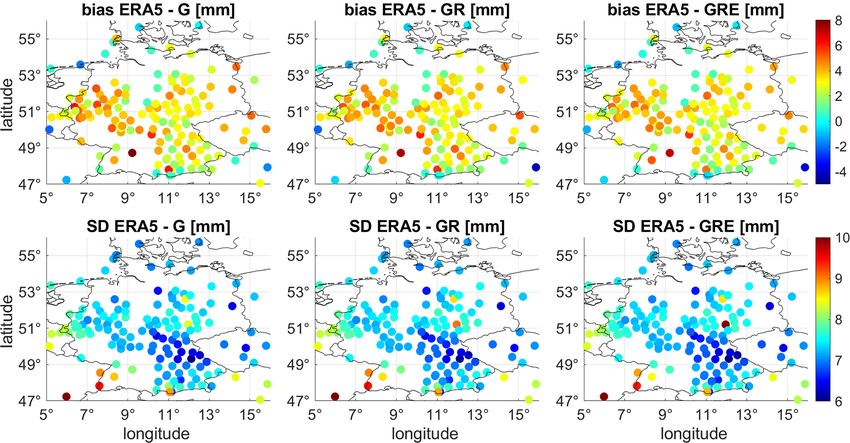
22                            K. Wilgan et al.: Towards operational multi-GNSS tropospheric products at GFZ Potsdam

Kawabata et al., 2013; Saito et al., 2017; Rohm et al., 2019).    et al., 2001; Teke et al., 2011; Wilgan et al., 2015; Douša
Nowcasting studies also show an improvement in forecasts,         et al., 2016; Hadaś et al., 2020; Lu et al., 2020; Bosser and
especially for water vapor while using the GNSS estimates         Bock, 2021), the tropospheric gradients (Li et al., 2015b; Lu
(Smith et al., 2000; Benevides et al., 2015; Benjamin et al.,     et al., 2016; Douša et al., 2017; Elgered et al., 2019; Kač-
2016).                                                            mařík et al., 2019) or STD (de Haan et al., 2002; Bender
   Some meteorological agencies such as the UK Met Of-            et al., 2008; Li et al., 2015a; Kačmařík et al., 2017). How-
fice, German Weather Service (DWD) or Japan Meteorolog-           ever, the majority of these studies are focused on the compar-
ical Agency (JMA) are operationally assimilating the GNSS         isons in the zenith direction, and the estimates were calcu-
tropospheric products. The challenge in the operational as-       lated from the GPS-only data, sometimes GPS–GLONASS
similation of the GNSS data is that the weather systems           combination. This study shows a comprehensive compari-
are already assimilating many observations from other data        son of all three tropospheric parameters, i.e., ZTDs, tropo-
sources. Thus, in the related assimilation studies, the impact    spheric gradients and STDs, with a main focus on the multi-
of GNSS data is reported just as slightly positive or neutral     GNSS estimates. It is also one of the first works showing
(Poli et al., 2007; Bennitt and Jupp, 2012; Lindskog et al.,      all three tropospheric parameters from multi-GNSS solution
2017). Moreover, these studies are only focused on the use        with fully operational Galileo constellation. A detailed com-
of tropospheric parameters in the zenith direction, i.e., ZTD     parison with some selected studies covering similar aspects
or IWV. More advanced products, such as tropospheric gra-         is shown in Sect. 5 – Discussion.
dients or slant total delays (STDs), are of interest, since in-      This Introduction is followed by Sect. 2 explaining the
formation on the horizontal distribution is provided by these     tropospheric parameters. Section 3 describes the GNSS and
parameters. A positive impact of the STD assimilation on          NWM data. Section 4 shows the comparison of three differ-
forecasts is to be expected, as it provides tropospheric infor-   ent tropospheric parameters, Sect. 5 discusses our findings in
mation in many different directions. The first assimilation ex-   view of the previous studies and the results are summarized
periments using tropospheric gradients were undertaken by         in Sect. 6.
Zus et al. (2019).
   This study is conducted within the recent research
project Advanced MUlti-GNSS Array for Monitoring Severe           2   Tropospheric parameters
Weather Events (AMUSE) of the German Research Founda-
                                                                  The microwave signals propagating through the atmosphere
tion (DFG). The main objectives of this project are (1) de-
                                                                  are delayed in its lowest part, the neutral atmosphere, which
velopments to provide high-quality slant tropospheric delays
                                                                  consists of the troposphere, stratosphere and a part of the
instead of only zenith delays, (2) developments to provide
                                                                  mesosphere (and is here called “troposphere” for shortness).
multi-GNSS products instead of GPS-only, (3) developments
                                                                  The delay is caused by the propagation medium, which is
to provide ultra-rapid tropospheric information and (4) mon-
                                                                  characterized by meteorological parameters: temperature, air
itoring and assimilation of the tropospheric products. Here,
                                                                  pressure and water vapor. The impact can be expressed by
we focus on the two first objectives. We show the compar-
                                                                  the refraction index n. Since this index is very close to unity,
isons of multi-GNSS tropospheric products, obtained using
                                                                  usually a parameter called total refractivity N is used (Essen
three satellite systems: the US American Global Navigation
                                                                  and Froome, 1951):
System (GPS), Russian GLONASS and European Galileo.
We calculate the tropospheric parameters from three sys-          N = 106 (n − 1).                                            (1)
tems for the stations located worldwide, with special em-
phasis on Germany using the in-house-developed software              The total refractivity can be calculated from the meteo-
Earth Parameter and Orbit determination System (EPOS.P8).         rological parameters using the following equation (Thayer,
We compare our estimates with the European Centre for             1974):
Medium-Range Weather Forecasts (ECMWF) ERA5 reanal-
ysis. The outcomes of this study will be assimilated in an op-             p − e −1    e          e −1
                                                                  N = k1        Zd + k2 Zv−1 + k3 2 Zw ,                      (2)
erational manner by the DWD. This study is thus a prepara-                   T         T         T
tion step for the assimilation that shows the tropospheric pa-    where p is the atmospheric air pressure (hPa); e is the
rameters from the operational software EPOS.P8 developed          water vapor partial pressure (hPa); T is the temperature
and run at GFZ. Moreover, the GFZ is one of the analysis          (K), k1 = 77.60 (K hPa−1 ), k2 = 70.4 (K hPa−1 ) and k3 =
centers for the EUMETNET EIG GNSS Water Vapour Pro-               373 900 (K hPa−2 ) are the refractivity coefficients, here taken
gramme (E-GVAP; http://egvap.dmi.dk/, last access: 17 De-         from Bevis et al. (1994); and Zd−1 and Zw   −1 are the inverse
cember 2021) and, as such, provides the ZTD and in the fu-        compressibility factors for dry air and water vapor, respec-
ture STD estimates to the weather agencies for the assimila-      tively, usually assumed to be 1.
tion.
   Many previous studies compared the tropospheric param-
eters from GNSS and NWM data for ZTD or IWV (Vedel

Atmos. Meas. Tech., 15, 21–39, 2022                                                   https://doi.org/10.5194/amt-15-21-2022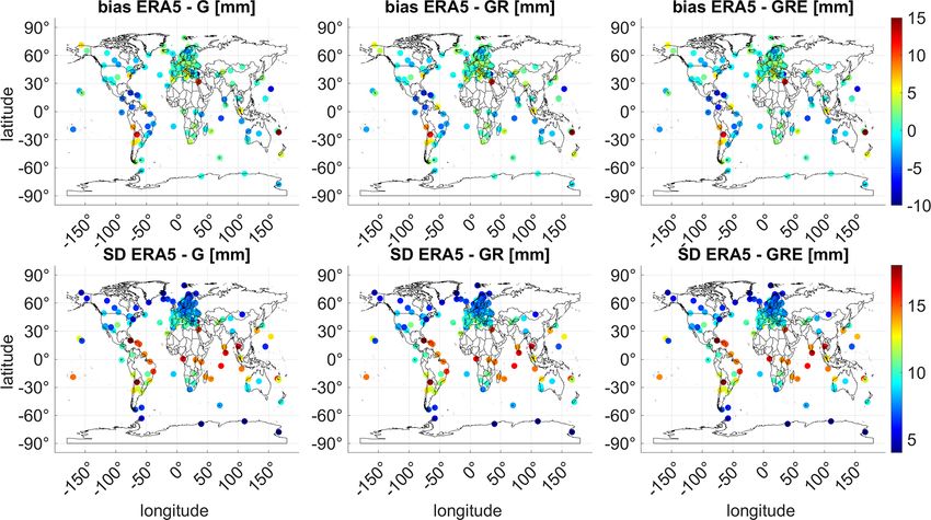
K. Wilgan et al.: Towards operational multi-GNSS tropospheric products at GFZ Potsdam                                            23

   From the total refractivity, a tropospheric delay in either    Table 1. Number of stations capable of receiving particular GNSS
the zenith (ZTD) or slant direction (STD) can be calculated:      signals used in this study.
           Z
1 = 10−6 N (s)ds + S − g,                                  (3)                              Whole world     Germany

             S                                                                  All                  663         313
                                                                                GRE                  376         152
where 1 denotes the delay, S denotes the arc-length of the                      GR only              251         152
ray path and g denotes the geometric distance between the                       G only                36           9
station and the satellite. In the GNSS analysis, the slant tro-
pospheric delay is approximated according to
                                                                  a priori ZHDs are taken from the Global Pressure Tempera-
STD = MFh (el) · ZHD + MFw (el) · ZWD
                                                                  ture 2 (GPT2) model (Böhm et al., 2007; Lagler et al., 2013),
       + MFg (el) [GN cos(A) + GE sin(A)] + res,           (4)    and the mapping function for the ZTD is the Global Mapping
                                                                  Function (GMF) (Böhm et al., 2006). The mapping func-
where ZHD and ZWD are the hydrostatic and wet parts of the
                                                                  tion for tropospheric gradients is calculated according to Bar-
ZTD, respectively; GN and GE denote the north–south and
                                                                  Sever et al. (1998); i.e., the wet mapping function is multi-
east–west gradient components; MFh , MFw and MFg are the
                                                                  plied by the cotangent of the respective elevation angle. More
mapping functions for the hydrostatic, wet part (e.g., Böhm
                                                                  processing information can be found in Table 2.
et al., 2006) and gradients (e.g., Bar-Sever et al., 1998; Chen
and Herring, 1997), respectively; el is the elevation angle; A    3.2   NWM data
the azimuth angle; and res is the post-fit phase residuals.
                                                                  The GNSS estimates are compared with the data from
                                                                  the fifth-generation ECMWF reanalysis (ERA5; http://www.
3     Data
                                                                  ecmwf.int/en/forecasts/datasets/reanalysis-datasets/era5, last
We have processed the initial data from three multi-GNSS          access: 17 December 2021). The ERA5 data are provided
solutions and ERA5 for the entire year of 2020. In this sec-      with a horizontal resolution of 0.25◦ × 0.25◦ on 31 pressure
tion, we describe the data sources in more detail.                levels. The data are provided with a 3-month delay; however
                                                                  the preliminary data sets are published with a delay of 5 d.
3.1    GNSS data                                                  The temporal resolution used in this study is 1 h for ZTDs
                                                                  and tropospheric gradients and 6 h for STDs (to reduce the
Our study incorporates GNSS data from three systems: GPS          computational cost and the data volume). There is no ground-
(G), GLONASS (R) and Galileo (E) for 663 stations world-          based GNSS data assimilation in the model, but the GNSS ra-
wide from the German national network SAPOS, the Inter-           dio occultation (RO) data are assimilated (Healy et al., 2005).
national GNSS Service (IGS; http://www.igs.org, last access:         The ERA5 provides gridded pressure, temperature and hu-
17 December 2021, Johnston et al., 2017) network, the EU-         midity fields. Hence, in the first step, the gridded refractiv-
REF Permanent Network (EPN; http://www.epncb.oma.be,              ity field is computed using Eq. (2). Then, the refractivity at
last access: 17 December 2021) and the GFZ network (Ra-           any arbitrary point is obtained by interpolation; i.e., for some
matschi et al., 2019). Unfortunately, not all used stations are   arbitrary point, the four surrounding refractivity profiles are
adapted to receive all types of GNSS signals yet. The num-        identified, and for each refractivity profile, a logarithmic in-
ber of stations capable of receiving particular signals for the   terpolation adjusts the refractivity vertically, and then a bilin-
whole world and specifically for Germany is given in Ta-          ear interpolation including the vertically adjusted refractivity
ble 1. Figure 1 shows the map of all stations for the whole       values is performed (Zus et al., 2012). This interpolation rou-
world and Fig. 2 for Germany. For most of our comparisons         tine is the prerequisite to the computation of the tropospheric
(for ZTDs and tropospheric gradients), we consider only the       delays for arbitrary station locations (Zus et al., 2014).
GRE-capable stations.                                                The STDs for each GNSS satellite–receiver pair are cal-
   The data are processed with the EPOS.P8 software devel-        culated using the GFZ-developed ray-tracing software de-
oped at GFZ (Dick et al., 2001; Gendt et al., 2004; Wickert       scribed in detail by Zus et al. (2014). The horizontal gra-
et al., 2020) in the post-processing mode using the precise       dients from the ERA5 are calculated by the least-squares
point positioning (PPP) technique. The tropospheric param-        adjustment. The used gradient mapping function is the one
eters are adjusted using the 24 h data intervals with the sam-    proposed by Bar-Sever et al. (1998) to match the gradient
pling rate of 15 min for ZTD and tropospheric gradients. The      mapping function that is utilized in the GNSS analysis. The
post-fit residuals are used for the calculation of STDs with      exact description of the methodology of calculating gradients
a 2.5 min sampling rate. In the preprocessing step, the GFZ       is presented by Zus et al. (2019).
high-quality orbits and clocks are estimated using a base of
approx. 100 stations located uniformly around the world. The

https://doi.org/10.5194/amt-15-21-2022                                                    Atmos. Meas. Tech., 15, 21–39, 2022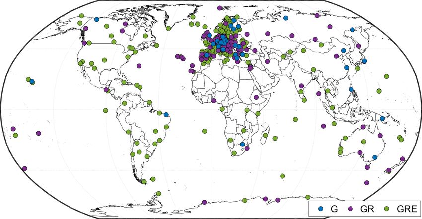
24                               K. Wilgan et al.: Towards operational multi-GNSS tropospheric products at GFZ Potsdam

Figure 1. Global map showing all stations used in this study. The colors indicate the capability to receive signals from the particular GNSS.

Table 2. Characteristics of the multi-GNSS processing at GFZ for this study.

      Processing         Description
      option
      Observations       Dual-frequency code and phase GPS L1/L2, GLONASS L1/L2 and Galileo E1/E5a observations
      Products           Precise orbits and Earth rotation parameters calculated using 100 global sites
      Observation        Elevation cutoff angle 7◦ , elevation-dependent weighting with unit weight above 30◦ , 1/2 sin(el) below 30◦
      handling           Undifferenced observations with 2.5 min sampling rate
      Antenna model      IGS14-2175 model (receiver and satellite phase center offsets and variations)
      Intersystem        Estimated as constant (per station and day), GPS as reference
      biases
      Troposphere        A priori GPT2 model with GMF for ZTD and Bar-Sever MF for gradients
                         Estimated ZTD and tropospheric gradients every 15 min; STDs every 2.5 min
                         Post-fit residuals applied
      Ionosphere         Eliminated using ionosphere-free linear combination
      Loading effects    Atmospheric tidal loading applied (S1 & S2 atmospheric pressure loading; Petit and Luzum, 2010)
                         Ocean tidal loading applied (FES2004)
                         Hydrostatic loading not applied
      Gravity            EGM2008 model

4    Results                                                             4.1     Comparisons of zenith total delays

We present the comparison of tropospheric parameters:                    At first, we show the intra-comparisons of the three GNSS
ZTDs, tropospheric gradients and STDs obtained from three                solutions, and then we compare the solutions with ERA5.
GNSS solutions with ERA5 estimates. We acknowledge that                  In the following comparisons, we take into account only the
the NWMs are an imperfect reference data source; however,                stations that are GRE compatible, i.e., 376 stations for the
their global coverage makes it convenient to see how the                 entire world and 152 for Germany.
agreement between them and the particular GNSS solutions
changes. The comparisons are made for the entire year of                 4.1.1    Intra-comparisons of the GNSS solutions
2020.
                                                                         We compare the GNSS estimates from the three solu-
                                                                         tions, GPS-only (G), GPS–GLONASS (GR) and GPS–
                                                                         GLONASS–Galileo (GRE). At first, we take a look at the for-

Atmos. Meas. Tech., 15, 21–39, 2022                                                           https://doi.org/10.5194/amt-15-21-2022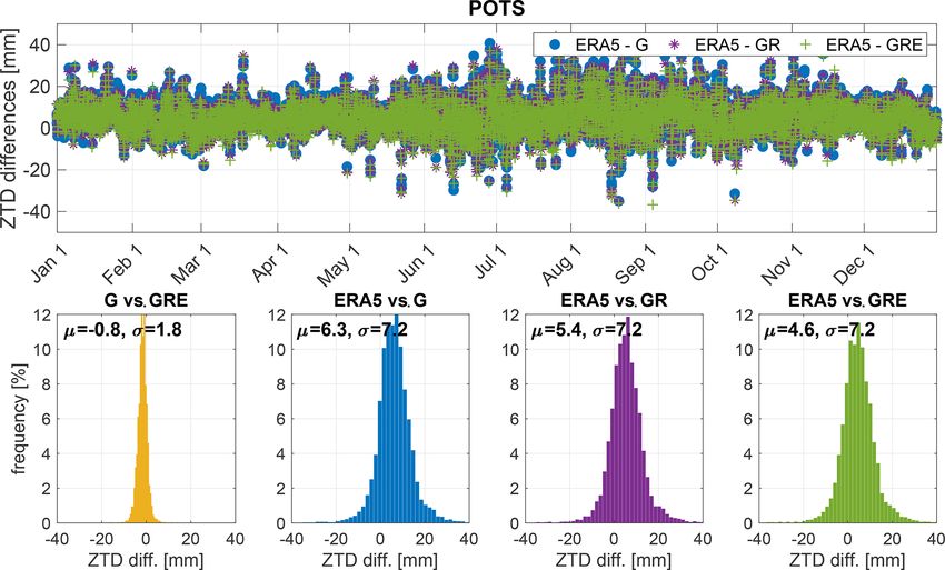
K. Wilgan et al.: Towards operational multi-GNSS tropospheric products at GFZ Potsdam 25
Table 4. Statistics between the ZTD from ERA5 and GNSS solu-
tions averaged from the year 2020 and all stations.
Whole world Germany only
(376 stations) (152 stations)
Comparison Bias SD Bias SD
(mm) (mm) (mm) (mm)
ERA5-G 1.72 8.64 2.93 7.34
ERA5-GR 1.86 8.57 2.94 7.35
ERA5-GRE 1.71 8.56 2.73 7.33
ences between ERA5 and the GNSS for each solution exhibit
similar patterns. However, the number of outliers is reduced
Figure 2. Map of the stations used for Germany. The colors indicate for the GR and GRE solutions compared to the GPS-only so-
the capability to receive signals from the particular GNSS. lution. It shows that the GR and GRE solutions are less noisy.
Table 4 shows the overall statistics of the differences between
ERA5 and particular GNSS solutions. Figure 6 shows the bi-
Table 3. Statistics between the particular GNSS ZTD solutions av-
eraged from all stations for the entire year of 2020. ases and SDs for each station between the ERA5 model and
GNSS solutions. For better visualization of the results, Fig. 7
Whole world Germany only shows the statistics for each station on a map for the entire
(376 stations) (152 stations) world and Fig. 8 for Germany.
Figure 6 shows that at the first glance, all three solutions
Comparison Bias SD Bias SD are very similar. However, taking a closer look to the statis-
(mm) (mm) (mm) (mm)
tics in Table 4 we can see some differences. For the whole
G-GR 0.13 1.71 0.02 1.50 world, the biases are similar for GPS-only and GRE solu-
G-GRE −0.04 1.99 −0.21 1.73 tions, while for GR they are slightly larger. The SDs are
GR-GRE −0.17 1.21 −0.22 1.06 slightly reduced for GR and GRE compared to the GPS-only
solution. For Germany, the GRE solution has the smallest
bias, but the SDs from all solutions are basically the same.
mal errors of ZTDs from the three solutions. Figure 3 shows Figure 7 shows the distribution of the biases and SDs on
the errors averaged for each station from the entire year of the world map. For the Northern Hemisphere, the biases are
2020 as well as one value for each system, averaged from all small and positive except for a few stations. The positive bias
the epochs and stations. We can see that adding GLONASS means that the ERA5 model is producing conditions that are
reduces the formal error from 1.22 to 0.99 mm, and adding too wet compared to the GNSS estimates. Close to the Equa-
Galileo reduces it further to 0.93 mm. tor, the biases are larger and negative. Here, the ERA5 model
Figure 4 shows the biases plus/minus their respective stan- is producing conditions that are too dry with respect to the
dard deviations (SDs) for each station (sorted by latitude, GNSS estimates. The pattern we find, i.e., the underestima-
Southern Hemisphere first), and Table 3 shows the mean bi- tion of the NWM delays around the Equator and the over-
ases and SDs averaged from all stations. estimation of the NWM delays at midlatitudes, is in good
Figure 4 shows that the largest differences can be observed agreement with the results reported by Bock and Parracho
for the Southern Hemisphere and around the Equator, where (2019). The SDs are also larger close to the Equator, where
the ZTD values are in general larger. The differences between the values of the ZTDs are in general larger due to higher
particular solutions are small but existent. Table 3 shows that humidity, which makes it more difficult to predict the values
the biases are the largest between GR and GRE solutions for from NWMs as well as estimate them with GNSS data.
the whole world, and between GPS and GRE, as well as be- Figure 8 shows larger, positive biases for the western part
tween GR and GRE for Germany. The SDs are the largest of Germany, while in the eastern part they are smaller. Only
between GPS and GRE in both cases. for a few stations are the biases negative. The SDs are almost
identical for most of Germany (about 6–8 mm). The differ-
4.1.2 Comparisons with NWMs ences between particular solutions are not large, but for some
stations, especially in the south and west of Germany, both
We compare the three GNSS solutions with the ERA5 esti- biases and SDs are slightly reduced for the GRE solution.
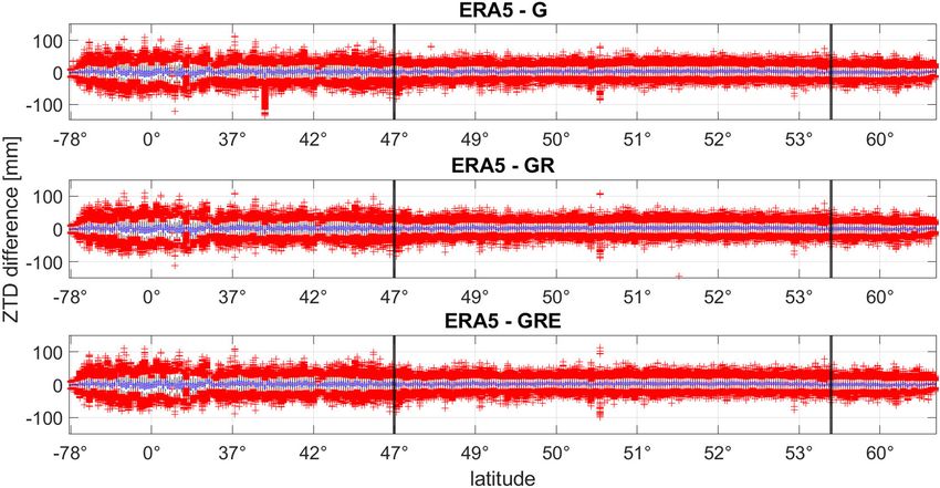
mates. Figure 5 shows the box plots of the differences be- Figures 9 and 10 show the ZTD differences between the three
tween the GNSS and ERA5. As shown in the plot, the differ- GNSS solutions and ERA5, as well as the histograms of the
https://doi.org/10.5194/amt-15-21-2022 Atmos. Meas. Tech., 15, 21–39, 2022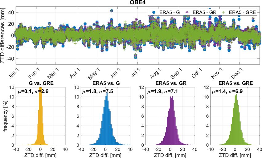
26                               K. Wilgan et al.: Towards operational multi-GNSS tropospheric products at GFZ Potsdam

Figure 3. Average formal errors of ZTD for each station in the processing (sorted by latitude, Southern Hemisphere first) (a) and the mean
formal error averaged from all stations and epochs (b). The red lines indicate the latitude band that includes Germany. Please note that the
labeling of the x axis is non-equidistant. The values are calculated for the year 2020.

Figure 4. The ZTD biases and SDs for each station (sorted by latitude, Southern Hemisphere first) between the three different GNSS
solutions. The red lines indicate the latitude band that includes Germany. Please note that the labeling of the x axis is non-equidistant. The
statistics are calculated for the year 2020.

residuals for two sample stations: POTS (Potsdam, Germany)               4.2    Comparisons of tropospheric gradients
and OBE4 (Oberpfaffenhofen, Germany), respectively.
   Both POTS and OBE4 have large, positive biases and SDs                The tropospheric gradients are a measure of anisotropy in the
with respect to the ERA5. For the station POTS (Fig. 9), we              north–south (GN ) and east–west (GE ) directions. The gradi-
can observe a reduction of bias of around 1.5 mm for GRE                 ents are of small magnitude, typically below 3 mm. Table 5
compared to the GPS-only solution, while the SDs remain at               shows the biases, SDs and Pearson’s correlation coefficients
the same level. For the station OBE4 (Fig.10) there is a small           (R) between the three GNSS solutions averaged from all the
reduction of both the biases and SDs.                                    stations and epochs, and Table 6 shows the same statistics but
                                                                         between ERA5 and the three GNSS solutions.
                                                                            As shown in Table 5, the biases between the particu-
                                                                         lar solutions are very close to zero, and SDs are of 0.1–
                                                                         0.2 mm. The largest SDs are between GRE and GPS-only

Atmos. Meas. Tech., 15, 21–39, 2022                                                            https://doi.org/10.5194/amt-15-21-2022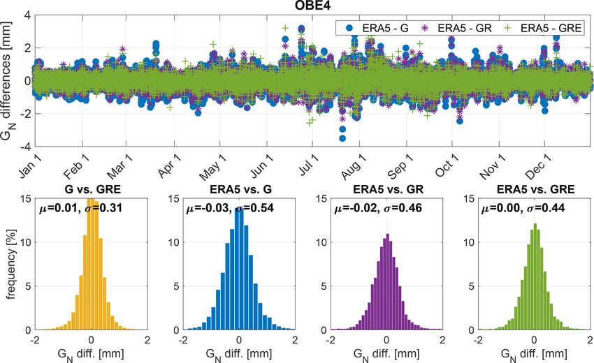
K. Wilgan et al.: Towards operational multi-GNSS tropospheric products at GFZ Potsdam                                                         27

Figure 5. The box plots of the ZTD differences between ERA5 and three GNSS solutions for each station. The blue boxes denote the 25th
and 75th percentile. The median is marked inside the boxes. The red crosses denote outliers. The stations are sorted by latitude, and the black
lines indicate the latitude band that includes Germany. Please note that the labeling of the x axis is non-equidistant. The values are calculated
for the year 2020.

Figure 6. The ZTD biases and SDs for each station (sorted by latitude, Southern Hemisphere first) between the ERA5 model and three
different GNSS solutions. The red lines indicate the latitude band that includes Germany. Please note that the labeling of the x axis is
non-equidistant. The statistics are calculated for the year 2020.

solutions, which was expected. For Germany, the SDs are                    rather small. Moreover, the differences between the particu-
slightly smaller than for the whole world. The correlations                lar GNSS solutions are not pronounced. The correlation co-
between the solutions are high, around 0.9–1.0, and are the                efficients are slightly higher for the GRE solution. For Ger-
highest between GR and GRE solutions and the lowest be-                    many, the biases are larger than for the entire world, but the
tween GPS-only and GRE.                                                    SDs are smaller. The correlation coefficients are also a bit
   The values in Table 6 are a few times larger than in Ta-                larger for Germany, where the gradients are more consistent.
ble 5. They may still seem small, but please note that, with               We do not show the plots analogical to Figs. 4 and 6 but
the exception of severe weather conditions, the values of gra-             would like to mention that the statistics (mostly SDs) are also
dients are usually below 1 mm. The SD of around 0.4 mm                     larger for the Southern Hemisphere and close to the Equator,
can actually constitute 40 % or more of the entire gradient                but the magnitude is smaller than for ZTDs. To give an exam-
value. Thus, the differences between ERA5 and GNSS gra-                    ple of the gradients’ behavior, we plot them for a sample sta-
dients are considered significant. The biases are however still            tion OBE4. Figure 11 shows the differences between ERA5

https://doi.org/10.5194/amt-15-21-2022                                                              Atmos. Meas. Tech., 15, 21–39, 2022
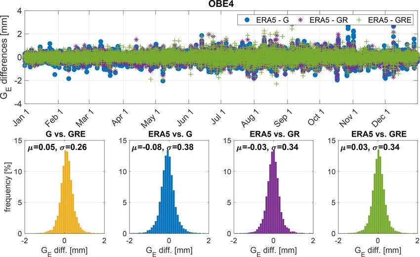
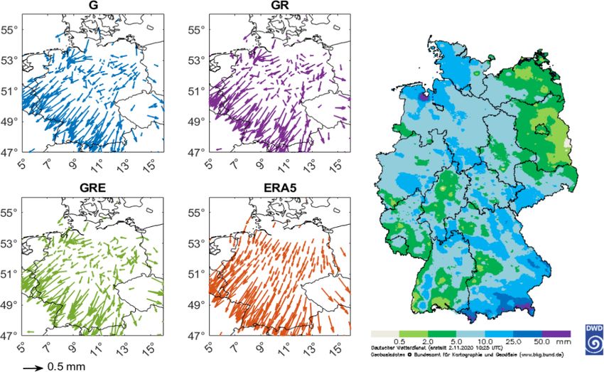
28                             K. Wilgan et al.: Towards operational multi-GNSS tropospheric products at GFZ Potsdam

Figure 7. The map of ZTD biases and SDs for each station between the ERA5 model and three different GNSS solutions. The statistics are
calculated for the year 2020.

Figure 8. The map of ZTD biases and standard deviations between ERA5 and the three GNSS solutions for Germany. The values are averaged
from the year 2020. The map shows only the GRE capable stations; thus there are gaps for some regions.

and GNSS for the north–south gradient and Fig. 12 for the               Both gradient components form a vector which points to
east–west gradient.                                                  the local maxima of tropospheric correction, and this usually
   Figures 11 and 12 do not show a visible offset between the        corresponds to the increasing water vapor content (Douša
ERA5 and GNSS values like in the case of ZTD. The tropo-             et al., 2016). To visualize that, Fig. 13 shows gradients for
spheric gradients, especially from the GNSS, are much more           one chosen date, 29 October 2020, 12:00 UTC. On that day,
varying and harder to predict than ZTDs. For this particular         a considerable amount of rain, especially in the southwest
station (OBE4), there is a slight reduction of bias and a larger     of Germany, was observed (up to 50 mm d−1 in southern
reduction of SD for the both GR and GRE solution compared            Bavaria). The figure also contains a map of the precipitation
to the GPS-only solution for GN , as well as a reduction of          for Germany on that day.
bias and SDs for the GE . This shows that for some particu-             The tropospheric gradients from ERA5, as shown in
lar stations, using more systems is more beneficial than just        Fig. 13, exhibit a clear pattern, pointing to the southeast di-
using GPS also for tropospheric gradients.                           rection for almost the entire country. The GNSS gradients ap-

Atmos. Meas. Tech., 15, 21–39, 2022                                                      https://doi.org/10.5194/amt-15-21-2022
K. Wilgan et al.: Towards operational multi-GNSS tropospheric products at GFZ Potsdam                                                 29

Figure 9. The ZTD difference values for station POTS (Potsdam, Germany) between the three GNSS solutions: GPS-only, GR and GRE and
ERA5 model (top) and histograms of the differences between the particular solutions and models (bottom). The plots are shown for the year
2020.

Figure 10. The ZTD difference values for station OBE4 (Oberpfaffenhofen, Germany) between the three GNSS solutions: GPS-only, GR and
GRE and ERA5 model (top) and histograms of the differences between the particular solutions and models (bottom). The plots are shown
for the year 2020.

pear more noisy, especially in northeastern Germany. How-              4.3   Comparisons of slant total delays
ever, all the GNSS solutions are very similar. In general, they
also point in the same direction as the ERA5 gradients, es-            From the information in the zenith direction, the tropospheric
pecially in southeastern Germany, where the gradient magni-            gradients and the post-fit residuals, the GNSS STDs are de-
tudes are much larger. For this part of the country, all the           rived (Eq. 4). We compare the STDs from the three GNSS so-
ERA5 gradients clearly changed direction, but the GNSS                 lutions with the ray-traced STDs from ERA5 model. Please
gradients do not reconstruct this behavior so clearly.                 note that due to the coarse temporal resolution of ERA5 and
                                                                       computational costs, the ray-traced STDs are calculated only
                                                                       four times per day. Moreover, we take the information from
                                                                       all the stations depicted in Figs. 1 and 2 (i.e., 663 stations for

https://doi.org/10.5194/amt-15-21-2022                                                         Atmos. Meas. Tech., 15, 21–39, 2022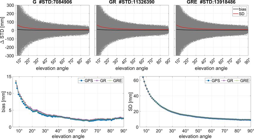
30                             K. Wilgan et al.: Towards operational multi-GNSS tropospheric products at GFZ Potsdam

Figure 11. The GN differences between the three GNSS solutions: GPS-only, GR and GRE and ERA5 for station OBE4 (Oberpfaffenhofen,
Germany) (top) and the histograms of the differences (bottom). The statistics were calculated from the year 2020.

Figure 12. The GE differences between the three GNSS solutions: GPS-only, GR and GRE and ERA5 for station OBE4 (Oberpfaffenhofen,
Germany) (top) and the histograms of the differences (bottom). The statistics were calculated from the year 2020.

the entire world and 313 stations for Germany) because for         that the number of observations is higher for GRE or GR than
STDs we have a separate solution for each satellite–station        for GPS-only, but the shape of the curves is very similar for
pair; thus there is no need to exclude any specific stations.      all three solutions. The average SDs are also almost identical
Figure 14 shows the differences between the three solutions        for all solutions; however, the biases differ slightly, with the
and the ERA5 estimates for each elevation angle and the            smallest biases obtained from the GPS-only and GRE solu-
statistics derived from the comparison.                            tions and the largest from GR.
   Figure 14 shows larger differences for low elevation an-           Table 7 shows the statistics for the entire world for the
gles than close to the zenith. This is due to the fact that the    differences between the GNSS solutions and ERA5 model.
STDs for low elevation angles (here the cutoff angle is 7◦ ) are   Due to the fact that the STD values are much larger for low
around 10 times larger than at zenith. Thus, also the residuals    elevation angles, we also show the statistics for the relative
for the low elevation angles are much larger. We can also see      differences (dSTDs), which are obtained by dividing the dif-

Atmos. Meas. Tech., 15, 21–39, 2022                                                    https://doi.org/10.5194/amt-15-21-2022
K. Wilgan et al.: Towards operational multi-GNSS tropospheric products at GFZ Potsdam                                              31

Figure 13. The tropospheric gradients from the three GNSS solutions and ERA5 for Germany for a chosen date: 29 October 2020, 12:00 UTC
(left panel). The right panel shows a map of precipitation for Germany on that day (source: DWD).

Figure 14. The STD differences between ERA5 and three GNSS solutions for the year 2020 for all 663 stations with marked average biases
and SDs (top) and the averaged biases and SDs from all solutions altogether (bottom).

ferences by the GNSS STD value as well as for the mapped             products that are extracted from the GRE solution. Table 9
ZTDs. These ZTDs are calculated using a simple 1/ sin(el)            shows the analogous parameters but averaged from the Ger-
mapping function; i.e., ZTD = sin(el) · STD. The simple MF           man stations.
is used here just to project the results to the zenith direction        As shown in Table 7, the agreement is at a similar level
to make them more comparable. To calculate the STDs, the             for all solutions. However, it is slightly worse for the GR
GMF is used as described in Sect. 3.1. Table 7 also consists         and GRE solutions, compared to GPS-only solution. If we
of the statistics for the GPS-, GLONASS- and Galileo-only            consider each system separately (from the GRE solution),

https://doi.org/10.5194/amt-15-21-2022                                                       Atmos. Meas. Tech., 15, 21–39, 2022
32                               K. Wilgan et al.: Towards operational multi-GNSS tropospheric products at GFZ Potsdam

Table 5. Biases, SDs and Pearson’s correlations between the three     and consequently the Galileo residuals are smaller and con-
GNSS solutions for tropospheric gradients averaged from the year      tain less noise. However, not all studies consistently conclude
2020 and all stations.                                                that post-fit residuals should be added when reconstructing
                                                                      the STDs (e.g., Zus et al., 2012; Kačmařík et al., 2017). The
                    Whole world                Germany only           post-fit residuals contain some tropospheric information, but
                    (376 stations)             (152 stations)
                                                                      the residuals can also be noisy, hence deteriorating the recon-
 Comparison      Bias      SD          R     Bias     SD         R    struction of STDs. To show the impact of the post-fit resid-
                (mm)     (mm)         (–)   (mm)    (mm)        (–)   uals, we calculate the STDs with and without the residuals
 GN                                                                   for the month of October 2020 for the GRE solution. Table 8
                                                                      shows the statistics for the two solutions.
 G-GR            0.00     0.19       0.93    0.00    0.18   0.93         Table 8 shows that the differences between ERA5 and
 G-GRE           0.01     0.23       0.91    0.01    0.21   0.91
                                                                      GNSS solutions are in general smaller without the post-fit
 GR-GRE          0.01     0.14       0.96    0.01    0.12   0.97
                                                                      residuals. This is due to two facts: (1) ERA5 has a sparse
 GE                                                                   horizontal resolution, so it does not resolve small-scale wa-
 G-GR            0.00     0.18       0.92    0.00    0.16   0.94      ter vapor well; and (2) residuals contain mostly noise, espe-
 G-GRE           0.00     0.23       0.88    0.01    0.20   0.91      cially for high elevation angles. However, in cases of severe
 GR-GRE          0.00     0.15       0.95    0.00    0.13   0.96      weather events, there may be more tropospheric information
                                                                      in the residuals, which can have more positive influence on
                                                                      the NWM assimilation. Thus, we keep the post-fit residu-
Table 6. Biases, SDs and Pearson’s correlations between the ERA5      als in our operational computations. Moreover, the usage of
and GNSS solutions for tropospheric gradients averaged from the       post-fit residuals has the largest impact on the Galileo so-
year 2020.
                                                                      lutions. We can see that when using the post-fit residuals,
                                                                      the bias for the Galileo-only solution is more significantly
                    Whole world                Germany only
                    (376 stations)             (152 stations)
                                                                      reduced compared to the solutions from other systems. For
                                                                      the solution without residuals, the biases for Galileo-only are
 Comparison       Bias     SD          R     Bias     SD         R    also reduced but less significantly. Thus, the post-fit residuals
                 (mm)    (mm)         (–)   (mm)    (mm)        (–)   from the Galileo system contain less noise and more informa-
 GN                                                                   tion than from the other systems.
 ERA5-G         −0.03     0.44       0.58   −0.05    0.40   0.61
                                                                         Table 7 also shows the total number of observations
 ERA5-GR        −0.03     0.44       0.59   −0.05    0.40   0.63      and detected outliers calculated using Chauvenet’s criterion.
 ERA5-GRE       −0.02     0.44       0.60   −0.04    0.39   0.64      Most of the outliers are found in the GRE solution for GPS
                                                                      observations, even though for the GPS-only processing there
 GE
                                                                      were not that many of them, which shows that processing
 ERA5-G         −0.01     0.38       0.57   −0.01    0.34   0.64      GPS-only data and extracting the GPS-only data from the
 ERA5-GR        −0.01     0.39       0.58   −0.01    0.35   0.65      GRE solution results in different estimates.
 ERA5-GRE       −0.01     0.39       0.58   −0.01    0.36   0.65         For Germany only, as shown in Table 9, we have slightly
                                                                      worse biases than for the whole world (because here the
                                                                      residuals mostly have the same sign, so the biases do not
we can see that actually the Galileo-only solution has the            cancel out), but the SDs are somewhat smaller. The statis-
smallest biases. The biases and SDs in Table 7 may appear             tics are following a similar pattern as for the entire world:
quite large, but when we calculate the average relative statis-       the best agreement is still for the GPS-only solution. How-
tics, the biases from different solutions are around 0.07 %           ever, for the separate systems in the GRE solution, the GPS
and SDs around 0.4 %. They are following the same patterns            has the best agreement and not Galileo as in the case of the
as the absolute statistics; i.e., the GPS-only solution has the       entire world. The statistics for the relative STDs and mapped
best agreement, but the bias is the smallest from the Galileo-        ZTDs do not show the same agreement as for the absolute
only solution. The biases for the mapped ZTDs are very sim-           STDs. Here, the biases for GPS-only and GRE solutions are
ilar to the ones presented in Sect. 4.1, but the SDs are a            more similar, and only for GR are they higher, while the SDs
bit larger. One reason is the usage of the simple 1/ sin(el)          are similar for GR and GRE. The reason may be that for GR
mapping function, which may deteriorate the results (She-             we have more observations for low elevation angles, which
haj et al., 2020). The other possible reason may be adding            being mapped with the simple MF can give larger discrepan-
the phase post-fit residuals, which may introduce more noise          cies.
to the solution. The usage of the post-fit residuals may also            Figure 14 shows that the differences between the ERA5
be the reason why the biases from Galileo-only solution are           and GNSS estimates depend strongly on the elevation angle.
the smallest. The Galileo clocks are more stable than GPS             To remove this dependence, we plot in Fig. 15 the relative
and GLONASS, which is beneficial for the PPP approach,                differences between the model and the GNSS solutions, as

Atmos. Meas. Tech., 15, 21–39, 2022                                                       https://doi.org/10.5194/amt-15-21-2022
K. Wilgan et al.: Towards operational multi-GNSS tropospheric products at GFZ Potsdam 33
Table 7. The STD biases and standard deviations between ERA5 and three GNSS solutions (whole world: 663 stations). The statistics are
calculated four times per day (at 00:00, 06:00, 12:00, and 18:00 UTC) and averaged over the year 2020.
Comparison Observations STD diff. dSTD diff. Mapped ZTD
(mm) (%) diff. (mm)
No. obs No. outliers Bias SD Bias SD Bias SD
ERA5-G 7 084 906 2511 4.18 26.25 0.076 0.408 1.81 9.54
ERA5-GR 11 326 390 4134 4.48 25.96 0.083 0.410 1.96 9.60
ERA5-GRE 13 918 486 5598 4.39 26.54 0.079 0.413 1.88 9.65
ERA5-GRE G only 6 479 156 2874 4.41 26.38 0.078 0.410 1.89 9.59
ERA5-GRE R only 4 569 105 1725 4.69 26.49 0.083 0.411 1.97 9.62
ERA5-GRE E only 2 870 225 999 3.86 26.97 0.072 0.421 1.71 9.84
Table 8. The STD biases and standard deviations between ERA5 and the GRE solution with and without post-fit residuals. The statistics are
calculated four times per day (at 00:00, 06:00, 12:00, and 18:00 UTC) and averaged over October 2020.
Comparison Observations STD diff. dSTD diff. Mapped ZTD
(mm) (%) diff. (mm)
No. obs No. outliers Bias SD Bias SD Bias SD
With post-fit residuals
ERA5-GRE 1 339 936 760 4.04 24.85 0.072 0.391 1.67 9.11
ERA5-GRE G only 605 052 422 4.09 25.12 0.070 0.389 1.62 9.07
ERA5-GRE R only 425 698 262 4.29 24.69 0.078 0.394 1.81 9.18
ERA5-GRE E only 309 186 76 3.57 24.51 0.068 0.390 1.58 9.08
Without post-fit residuals
ERA5-GRE 1 242 557 398 4.01 23.02 0.071 0.351 1.64 8.17
ERA5-GRE G only 561 284 232 4.17 23.34 0.072 0.352 1.67 8.21
ERA5-GRE R only 397 744 121 4.01 22.61 0.072 0.347 1.69 8.07
ERA5-GRE E only 283 529 45 3.71 22.95 0.066 0.354 1.53 8.24
well as the number of observations for each elevation angle for GRE. The STDs depend not only on the elevation angle,
batch. but also on the azimuth angle of the satellite (see Eq. 4). Fig-
Figure 15 shows that the relative differences are almost in- ure 16 shows the relative differences with respect to the az-
dependent from the elevation angle, which means that the so- imuth angle and the number of observations for each angle
lutions are of equal quality for all angles. Only close to zenith bin.
do the solutions tend to deteriorate due to the limited num- Figure 16 shows that the relative differences depend on the
ber of observations for such angles. The differences between azimuth angle, especially for the GPS-only solution and low
the solutions are rather small as shown in Table 7. Further- azimuth angles. The reason is, as shown in the bottom panel,
more, one of the advantages of combining the solutions is that there are only very few observations for azimuth angles
the increase of the number of observations. Figure 15 shows close to 0. Adding GLONASS and Galileo observations fills
that adding particular systems increases the number of ob- this gap a little and makes the differences less dependent on
servations significantly. For this yearly comparison with 6 h the azimuth angle. Thus, adding more systems to the solution
resolution, we use over 7 million GPS, 4 million GLONASS increases not only the number of low elevation angle obser-
and 3 million Galileo observations. Thus, the total number vations but also low azimuth angle, making the observations
of GRE observations has doubled compared to the GPS-only more uniformly distributed. To sum up, we can conclude that
observations. It is especially important that the number of even though adding more systems does not significantly im-
observations for lower elevation angles is increased. For the prove the agreement between the GNSS and ERA5 solutions,
lowest bin in Fig. 15, there are around 110 000 observations it increases the number of observations, especially for low el-
for GPS, 170 000 for GR and 230 000 observations for GRE. evation and azimuth angles. This addition may lead to more
But also the middle bins are significantly improved, from precise information about the tropospheric state obtained via,
around 100 000 observations for GPS-only to around 250 000 e.g., water vapor tomography.
https://doi.org/10.5194/amt-15-21-2022 Atmos. Meas. Tech., 15, 21–39, 202234 K. Wilgan et al.: Towards operational multi-GNSS tropospheric products at GFZ Potsdam
Table 9. The STD biases and standard deviations between ERA5 and different GNSS solutions (for Germany: 313 stations). The statistics
are calculated four times per day (at 00:00, 06:00, 12:00, and 18:00 UTC) and averaged over the year 2020.
Comparison Observations STD diff. dSTD diff. Mapped ZTD
(mm) (%) diff. (mm)
No. obs No. outliers Bias SD Bias SD Bias SD
ERA5-G 3 560 900 70 6.13 23.80 0.110 0.356 2.60 8.38
ERA5-GR 5 822 589 141 6.27 23.63 0.114 0.361 2.69 8.50
ERA5-GRE 7 005 028 218 6.26 24.01 0.111 0.360 2.63 8.47
ERA5-GRE G only 3 275 375 73 6.21 23.85 0.110 0.359 2.61 8.44
ERA5-GRE R only 2 459 968 54 6.30 24.17 0.111 0.363 2.62 8.55
ERA5-GRE E only 1 269 776 91 6.32 24.12 0.115 0.359 2.70 8.41
Figure 15. The STD relative differences between ERA5 and the three different GNSS solutions: GPS-only, GR and GRE (top panels) and
the number of observations with respect to the elevation angle for each solution (bottom). The differences are calculated for the entire year
of 2020.
5 Discussion very close to 0, with a SD of 0.4 mm, and for the GE gra-
dient, it was −0.05 mm, with a SD of 0.4 mm. The SDs in
Comparisons of the GNSS and NWM estimates have already this study correspond with the Repro2 study by Douša et al.
been vastly described in the literature. The majority of the (2017); however, our GN absolute biases are slightly larger
studies focus on the parameters in the zenith direction, either (−0.03 mm), and the GE biases are smaller (−0.01 mm).
ZTDs or IWV. Examples have been given in the Introduction Kačmařík et al. (2019) studied different settings of tropo-
of this article. Some of these studies have been conducted spheric gradients for a COST Action ES1206 benchmark pe-
at GFZ or use the GFZ products. In this section, we would riod (May–June 2013) for 430 stations in central Europe. The
like to summarize a few selected studies and compare our settings included eight different variants of processing gradi-
outcomes with theirs. ents with different mapping functions, elevation cutoff an-
Douša et al. (2017) compared the tropospheric GPS-only gle, GNSS constellation, observations’ elevation-dependent
products calculated at 172 stations from almost 20 years of weighting and the processing mode. One of the variants con-
data (1996–2014) of the second EUREF reprocessing (Re- cerned the GPS-only vs. the GPS–GLONASS solutions. The
pro2). The ZTD comparisons with ERA-Interim reanalysis comparison with the NWM showed that a small decrease in
for almost all variants showed biases of 2 mm and SDs of the SD of the estimated gradients (2 %) was observed when
8 mm, which exactly corresponds with the findings of this using GPS–GLONASS instead of GPS-only. In our study,
study for the whole world. For Germany only, the biases are there is no general improvement while taking the GR or GRE
3 mm with 7 mm SDs. For the GN gradient, the bias was solutions with respect to the GPS-only solutions. However,
Atmos. Meas. Tech., 15, 21–39, 2022 https://doi.org/10.5194/amt-15-21-2022K. Wilgan et al.: Towards operational multi-GNSS tropospheric products at GFZ Potsdam 35 Figure 16. The STD relative differences between ERA5 and the three different GNSS solutions: GPS-only, GR and GRE (top panels) and the number of observations with respect to the azimuth angle for each solution (bottom). The differences are calculated for the entire year of 2020. some selected stations, e.g., OBE4, showed a decrease of the SD of 1.95 mm between the solutions, which is very similar SDs. Lu et al. (2016) compared gradients from multi-GNSS to the current study. GFZ also provided their contribution to solution validated with the ECMWF NWM from 120 stations the study of Kačmařík et al. (2017), although at that time with for 3 months in 2014. At that time, only eight Galileo satel- a GPS-only solution. This was compared to the NWMs (the lites were in use. The results demonstrated that GLONASS GFS and ERA-Interim models). The biases for the mapped gradients achieved comparable accuracy to the GPS gradi- ZTDs varied for different stations between 4–12 mm with ents but had slightly more noise and outliers. Compared to SDs of 7–12 mm for GFS and 0–6 mm with 10–17 mm SDs the GPS- and GLONASS-only estimates, the correlation for for ERA5. The agreement is worse than in the current study the multi-GNSS processing was improved by about 21.1 % (for Germany, the mapped ZTDs biases are 3 mm with SDs and 26.0 %, respectively. These results do not correspond of 7.5 mm), probably due to the usage of the data in the warm fully with the findings of our study, where the gradients from season (and not the entire year like in this study) and possibly all three solutions exhibit a similar level of agreement with also due to the different way of calculating the STDs from the NWM. The correlation between GNSS and NWM data NWMs (the assembled and not the ray-traced tropospheric is improved by only 3 % for GRE compared to GPS-only so- delays were utilized). The study of Kačmařík et al. (2017) lution. The reason for higher reduction in these studies and also showed the impact of using the post-fit residuals. The smaller reduction in our study is most probably the usage SDs between the solution with and without residuals were of different ways of constraining the parameters. Kačmařík at a level of 4 mm with almost zero bias. In our study, we et al. (2019) and Lu et al. (2016) used loose constraining, calculate the statistics between the ERA5 and the two solu- while in our study the gradients are more tightly constrained tions. They show that the impact of the post-fit residuals is between epochs but more loose in the general magnitude. somehow smaller and that the biases differ only by less than Kačmařík et al. (2017) showed the comparisons of STDs 0.5 mm and the SDs by about 2 mm. from seven different institutions. The authors validated 11 Li et al. (2015a) described real-time comparisons of ZTDs, solutions obtained using five different GNSS processing soft- gradients, STDs and IWVs from 100 globally distributed sta- ware packages. They checked different processing strategies, tions and a 180 d period in 2014 and compared them to the elevation cutoff angle, mapping functions, products used, in- ECMWF operational analysis. In this study, the data from tervals of calculating the parameters or the usage of post-fit four systems were considered: GPS, GLONASS, Galileo and residuals. The tests were performed for 10 reference stations Beidou (GREC). However, the Galileo data were very lim- of the COST Action ES1206 benchmark in 2013. This study ited; there were only four satellites in the constellation. Our was restricted to GPS-only and GPS–GLONASS solutions. study is an extension of this previous study with a fully devel- Amongst the comparisons of many different aspects, it also oped Galileo constellation. Moreover, Li et al. (2015a) used showed that changing the setting from GPS-only to GPS– real-time PANDA software, while we use the operational GLONASS resulted in the mapped ZTD bias of 0.18 mm and EPOS.P8 software. The ECMWF vs. GREC ZTD compar- https://doi.org/10.5194/amt-15-21-2022 Atmos. Meas. Tech., 15, 21–39, 2022
36                             K. Wilgan et al.: Towards operational multi-GNSS tropospheric products at GFZ Potsdam

isons resulted in a fractional bias of 0.1 % and SD of 0.5 %        SDs of 0.4 mm and for GE the bias of −0.01 mm with 0.4 mm
(corresponding to around 2 and 12 mm), which is a bit worse         SDs. For Germany, the behavior was similar to the ZTDs’;
than in the current study (with the biases of also 2 mm and         i.e., the biases were slightly larger and SDs smaller. For
SDs of 8.5 mm). For gradients (although calculated every            STDs, the differences were strongly dependent on the ele-
12 h, not every 15 min like in this study), the authors cal-        vation angle, with larger differences for low elevation an-
culated the root-mean-square error (RMSE), which equaled            gles and smaller values close to the zenith. The average bias
0.34 mm for GREC and 0.38 mm for GPS-only, which was                was around 4 mm with 26 mm SDs, which corresponds to
an 11.8 % improvement. We do not see such a behavior for            0.08 % with 0.4 % SDs for the relative values. Unfortunately,
our gradients; they are at a similar level for all solutions. The   for STDs, adding GLONASS and Galileo did not improve
reason may again be that the gradients from Li et al. (2015a)       the agreement but even slightly worsened it. However, if we
are very loosely constrained, like in Kačmařík et al. (2019)      consider only the Galileo observations in the GRE solution,
and Lu et al. (2016), and this is not the case for our analy-       the bias was slightly reduced. For Germany, the statistics
sis. For the STDs, the authors do not give specific numbers,        were again worse for biases and better for SDs. We also an-
but visually the GPS-only and GREC solutions are close to           alyzed the relative differences between GNSS and ERA5 es-
each other. The SDs equaled approx. 1 cm close to the zenith        timates. The dependence on the elevation angle was reduced
and 10 cm at 7◦ , which corresponds with the findings of this       almost to zero. For the relative differences, the worst agree-
paper.                                                              ment was obtained for the values close to the zenith, where
   This study is generally in agreement with the findings           there are fewer observations. Moreover, the dependence on
of the described previous studies. The differences between          the azimuth angle was tested. For the GPS-only solution,
NWMs and the tropospheric delays, i.e., ZTDs and STDs, are          there was a deterioration of the agreement with ERA5 for
comparable. The main difference concerns the multi-GNSS             azimuth angles close to zero, where there were not so many
gradients, which is most likely due to the different ways           data. Adding GLONASS and Galileo increased the number
of constraining the gradient values. In the previous studies,       of observations for such low azimuth angles and resulted in
mostly the estimates from GPS and GLONASS were con-                 better agreement for these angles. In conclusion, the esti-
sidered, while this study additionally uses the fully opera-        mates from all three solutions showed a very similar agree-
tional Galileo constellation. Moreover, the software used in        ment with respect to the ERA5. We conclude that they are of
this study (EPOS.P8) is used to provide the tropospheric pa-        similar quality. Nonetheless, adding more systems results in
rameters to the weather services in an operational way.             better sky coverage, especially for low elevation and azimuth
                                                                    angles, which leads to a better geometry for future assimila-
                                                                    tion and tomography studies.
6    Summary

This study presented a comparison of tropospheric param-            Code availability. The GNSS data are processed using the GFZ-
eters: ZTDs, tropospheric gradients and STDs from three             developed software EPOS.P8. GFZ owns the intellectual property
GNSS solutions – GPS-only, GPS–GLONASS and GPS–                     rights to the EPOS.P8 software.
GLONASS–Galileo with the global ERA5 reanalysis. The
GNSS estimates were calculated using the GFZ-developed
software EPOS.P8, providing the parameters to the weather           Data availability. The ECMWF provided the ERA5 data (https:
                                                                    //www.ecmwf.int/en/forecasts/datasets/reanalysis-datasets/era5,
services operationally (e.g., DWD, Met Office). The three
                                                                    Zus, 2021). The GNSS observation data are provided by the
tropospheric parameters calculated using EPOS.P8 software           following global networks: IGS (http://www.igs.org, IGS,
and the full Galileo constellation were presented in a publi-       2021), EPN (http://www.epncb.oma.be, EPN, 2021) and
cation for the first time. For the ZTDs, the formal error was       GFZ       (https://doi.org/10.5880/GFZ.1.1.2020.001,   Ramatschi
reduced from 1.22 mm for GPS-only solution to 0.93 mm               et al., 2019). The station and satellite metadata are taken
for GRE. Global comparisons with ERA5 showed biases of              from the GFZ SEnsor Meta Information SYStem (SEMISYS,
around 2 mm with 8.5 mm SDs. The comparisons for Ger-               https://doi.org/10.5880/GFZ.1.1.2020.005, Bradke, 2020). The
many resulted in biases of 3 mm and SDs of 7 mm, which is           GNSS analysis results from this study can be made available upon
to be expected as for Germany the biases do not cancel out          request.
as in the case of the global network, but the estimates are
more consistent. All three GNSS solutions were very simi-
lar; however, the statistics were slightly better for the GRE       Author contributions. All authors contributed to the conceptualiza-
solution. There are some stations, e.g., POTS or OBE4, for          tion of this study. The methodology was provided by KW, GD and
                                                                    FZ. KW and FZ validated the results. The investigations were per-
which adding GLONASS and further Galileo reduced the bi-
                                                                    formed by KW, GD and FZ. Data curation was done by GD and FZ.
ases and SDs. For the tropospheric gradients, the results from      The original draft was written by KW and reviewed by JW, FZ and
all solutions were almost identical. For GN and the global          GD. The visualizations were made by KW and FZ. The project was
comparisons, the average bias was of around −0.03 mm with

Atmos. Meas. Tech., 15, 21–39, 2022                                                      https://doi.org/10.5194/amt-15-21-2022
K. Wilgan et al.: Towards operational multi-GNSS tropospheric products at GFZ Potsdam 37
administrated by JW, and the funding was acquired by JW and GD. and ERA-Interim reanalysis, Atmos. Chem. Phys., 19, 9453–
All authors read and approved the final paper. 9468, https://doi.org/10.5194/acp-19-9453-2019, 2019.
Böhm, J., Niell, A., Tregoning, P., and Schuh, H.: Global Map-
ping Function (GMF): A new empirical mapping function based
Competing interests. The contact author has declared that neither on numerical weather model data, Geophys. Res. Lett., 33, 3–6,
they nor their co-authors have any competing interests. https://doi.org/10.1029/2005GL025546, 2006.
Böhm, J., Heinkelmann, R., and Schuh, H.: Short note: A global
model of pressure and temperature for geodetic applications,
Disclaimer. Publisher’s note: Copernicus Publications remains J. Geodesy, 81, 679–683, https://doi.org/10.1007/s00190-007-
neutral with regard to jurisdictional claims in published maps and 0135-3, 2007.
institutional affiliations. Boniface, K., Ducrocq, V., Jaubert, G., Yan, X., Brousseau, P., Mas-
son, F., Champollion, C., Chéry, J., and Doerflinger, E.: Im-
pact of high-resolution data assimilation of GPS zenith delay
on Mediterranean heavy rainfall forecasting, Ann. Geophys., 27,
Acknowledgements. This study was performed under the frame-
2739–2753, https://doi.org/10.5194/angeo-27-2739-2009, 2009.
work of the Deutsche Forschungsgemeinschaft (DFG) project Ad-
Bosser, P. and Bock, O.: IWV retrieval from ground GNSS
vanced MUlti-GNSS Array for Monitoring Severe Weather Events
receivers during NAWDEX, Adv. Geosci., 55, 13–22,
(AMUSE), grant no. 418870484.
https://doi.org/10.5194/adgeo-55-13-2021, 2021.
Bradke, M.: SEMISYS – Sensor Meta Information
System, V. 4.1, GFZ Data Services [data set],
Financial support. This research has been supported by the https://doi.org/10.5880/GFZ.1.1.2020.005, 2020.
Deutsche Forschungsgemeinschaft (grant no. 418870484). Chen, G. and Herring, T. A.: Effects of atmospheric az-
imuthal asymmetry on the analysis of space geode-
tic data, J. Geophys. Res.-Sol. Ea., 102, 20489–20502,
Review statement. This paper was edited by Roeland Van Malderen https://doi.org/10.1029/97jb01739, 1997.
and reviewed by three anonymous referees. Cucurull, L., Derber, J. C., Treadon, R., and Purser, R. J.:
Assimilation of Global Positioning System Radio Oc-
cultation Observations into NCEP’s Global Data As-
similation System, Mon. Weather Rev., 135, 3174–3193,
References https://doi.org/10.1175/MWR3461.1, 2007.
de Haan, S., van der Marel, H., and Barlag, S.: Comparison of GPS
Bar-Sever, Y. E., Kroger, P. M., and Borjesson, J. A.: Estimat- slant delay measurements to a numerical model: case study of a
ing horizontal gradients of tropospheric path delay with a sin- cold front passage, Phys. Chem. Earth Pt. A/B/C, 27, 317–322,
gle GPS receiver, J. Geophys. Res.-Sol. Ea., 103, 5019–5035, https://doi.org/10.1016/S1474-7065(02)00006-2, 2002.
https://doi.org/10.1029/97jb03534, 1998. Dick, G., Gendt, G., and Reigber, C.: First experience
Bender, M., Dick, G., Wickert, J., Schmidt, T., Song, S., Gendt, G., with near real-time water vapor estimation in a German
Ge, M., and Rothacher, M.: Validation of GPS slant delays using GPS network, J. Atmos. Sol.-Terr. Phy., 63, 1295–1304,
water vapour radiometers and weather models, Meteorol. Z., 17, https://doi.org/10.1016/S1364-6826(00)00248-0, 2001.
807–812, https://doi.org/10.1127/0941-2948/2008/0341, 2008. Douša, J., Dick, G., Kačmařík, M., Brožková, R., Zus, F., Brenot,
Benevides, P., Catalao, J., and Miranda, P. M. A.: On the in- H., Stoycheva, A., Möller, G., and Kaplon, J.: Benchmark
clusion of GPS precipitable water vapour in the nowcast- campaign and case study episode in central Europe for de-
ing of rainfall, Nat. Hazards Earth Syst. Sci., 15, 2605–2616, velopment and assessment of advanced GNSS tropospheric
https://doi.org/10.5194/nhess-15-2605-2015, 2015. models and products, Atmos. Meas. Tech., 9, 2989–3008,
Benjamin, S. G., Weygandt, S. S., Brown, J. M., Hu, M., Alexander, https://doi.org/10.5194/amt-9-2989-2016, 2016.
C. R., Smirnova, T. G., Olson, J. B., James, E. P., Dowell, D. C., Dousa, J., Vaclavovic, P., and Elias, M.: Tropospheric products of
Grell, G. A., Lin, H., Peckham, S. E., Smith, T. L., Moninger, W. the second GOP European GNSS reprocessing (1996–2014), At-
R., Kenyon, J. S., and Manikin, G. S.: A North American hourly mos. Meas. Tech., 10, 3589–3607, https://doi.org/10.5194/amt-
assimilation and model forecast cycle: The Rapid Refresh, Mon. 10-3589-2017, 2017.
Weather Rev., 144, 1669–1694, https://doi.org/10.1175/MWR- Elgered, G., Ning, T., Forkman, P., and Haas, R.: On the infor-
D-15-0242.1, 2016. mation content in linear horizontal delay gradients estimated
Bennitt, G. V. and Jupp, A.: Operational assimilation of GPS zenith from space geodesy observations, Atmos. Meas. Tech., 12, 3805–
total delay observations into the Met Office numerical weather 3823, https://doi.org/10.5194/amt-12-3805-2019, 2019.
prediction models, Mon. Weather Rev., 140, 2706–2719, 2012. EPN: Daily GNSS data, EUREF Permanent Network, available at:
Bevis, M., Businger, S., Chiswell, S., Herring, T., Anthes, http://www.epncb.oma.be, last access: 5 November 2021.
R., Rocken, C., and Ware, R.: GPS meteorology: Map- Essen, L. and Froome, K.: The refractive indices and dielectric con-
ping zenith wet delays onto precipitable water, J. Appl. stants of air and its principal constituents at 24 000 Mc/s, P. Phys.
Meteorol., 33, 379–386, https://doi.org/10.1175/1520- Soc. Lond. B, 64, 862–875, https://doi.org/10.1038/167512a0,
0450(1994)0332.0.CO;2, 1994. 1951.
Bock, O. and Parracho, A. C.: Consistency and representativeness
of integrated water vapour from ground-based GPS observations
https://doi.org/10.5194/amt-15-21-2022 Atmos. Meas. Tech., 15, 21–39, 2022You can also read