Turbulence parameter estimation with Paranal Observatory wavefront sensors
←
→
Page content transcription
If your browser does not render page correctly, please read the page content below
25/10/2020
Turbulence parameter
estimation with Paranal
Observatory wavefront sensors
P.J.V. Garcia, P.P. Andrade, J. Kolb, J. Milli, C. Correia, M.I. Carvalho
pgarcia@fe.up.pt
“Wavefront sensing in the VLT/ELT era & AO Workshop Week II”, 13th ‐15th October 2020
1
1
Estimation of r0 and L0
• Site evaluation and characterization
• Observation scheduling
• Optimization of AO systems, including temporal updates
• Predictions of point spread functions (with or without AO)
• Optimization of fringe‐trackers for optical interferometry
• Addressed by many dedicated experiments
• Balloons, DIMM, MASS, SLODAR, SCIDAR, …
• Advantages of estimation using Shack‐Hartman WFS
• Ubiquity in large telescopes make use of existing infrastructure
• Spatio‐temporal synchronism
• Identical turbulence path (including dome‐telescope seeing) of the observations
• Previous work
• Single sensor: Schöck+2003, Fusco+2004, Jolissaint+2018
• Multiple sensor: Wilson+2002, Guesalaga+2017, Ono+2017
2
2
1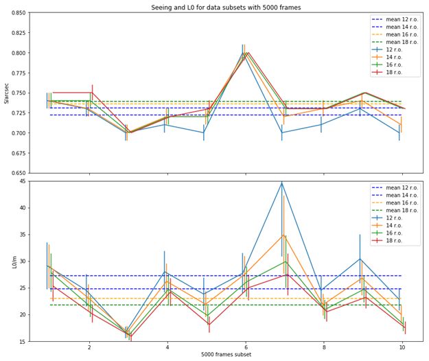
25/10/2020
Cross‐coupling is unavoidable in model fitting
• A Shack‐Hartmann is a “gradient” sensor
• The Zernike gradients matrix is non‐orthogonal cross‐coupling
• r0 and L0 are estimated using Zernike variances
• Diagonalizing the Zernike co‐variance matrix (using Karhunen‐Loève
basis) would not solve the problem
• No fitting functions for the r0 and L0 exist in this basis
• Statistical independence versus geometric coupling
• Cross‐coupling is unavoidable in r0 and L0 joint estimation with
model fitting
3
3
Overcoming cross‐coupling Andrade+2019
• Include cross‐coupling and noise in the model for
measured variances
• true variances, noise and cross coupling (can be
negative!)
• It turns out that the cross‐coupling contribution is
analytic (cf. Conan 2000, Takato+1995)
• but a function of r0 and L0 iterative method
4
4
2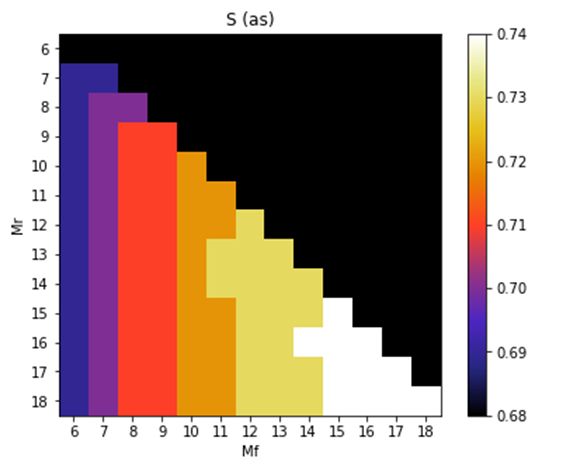
25/10/2020
Iterative method (Andrade+2019)
• Iteration zero is classic approach, obtain biased estimates of r0 and L0
• Remaining iterations include cross‐coupling correction
• estimating improved r0, L0 and noise 2 at each k
5
5
What about real data?
6
6
325/10/2020
Shack‐Hartman WFSs at Paranal: +13!
CIAO #3
CIAO #2 SAXO
CIAO #4
AOF #1‐#4
CIAO #1
NAOMI #3
NAOMI #1
NAOMI #2
NAOMI #4
7
7
Shack‐Hartman WFSs at Paranal
• SAXO
• 40x40 WFS, visible, control in Karhunen‐Loève modes
• CIAO #1‐#4
• 9x9 WFS, K‐band, control in Karhunen‐Loève modes, Coudé focus (rotation)
• NAOMI #1‐#4
• 4x4 WFS, visible, control in Zernike modes, Coudé focus (rotation)
• AOF #1‐#4
• 40x40 WFS, visible, Karhunen‐Loève modes
8
8
425/10/2020
Estimating r0 and L0 from real data
• Open loop
• Pros: simple
• Cons: uses science time
• Method
• Slopes to Zernike matrix is a geometric
model
• Convert to Zernike coefficients
• Apply fitting to variances
• Closed loop
• Pros: runs parallel to science
• Cons: complex combines voltages + slopes
• Method
• Define where to work (DM or WFS)
• Convert voltages or slopes
• Convert to Zernike coefficients
• Apply fitting to variances
9
9
AOF data |
non‐iterative (current method, left) versus iterative approach (right)
Results don’t depend on the number of radial orders in the reconstructor and slightly
depend on the number of orders in the fit. 10
10
525/10/2020
AOF data | snapshots of temporal evolution
11
11
The curse of high precision
• We are extremely precise in the estimation of r0 and L0
• This does not make sense physically
• Von Kármán is an approximation of turbulence in one layer
• Cf. literature on deviations from von Kármán (e.g. Goodwin+2016, Gueselaga+2014,
Lombardi+2010)
• What we measure is an average of several layers across the atmosphere
• Cf. next other talks in the present session!
• Non‐stationarity and correlation of the phase during measurements
• However temporal evolution opens up several possibilities.
12
12
625/10/2020
Future prospects & challenges
• Short term
• Work on closed loop data issues…
• Run pipeline on archived data
• Paranal turbulence parameters
• How does the estimation change with WFS characteristics?
• How does r0 and L0 change from telescope to telescope?
• Can we have a picture of these parameters on the mountain top
(position/height)?
• Non‐stationarity effects, SPARTA implementation, etc
• Telemetry data curation
• Stay tuned …
13
13
7You can also read