Upwelling-induced trace gas dynamics in the Baltic Sea inferred from 8 years of autonomous measurements on a ship of opportunity
←
→
Page content transcription
If your browser does not render page correctly, please read the page content below
Biogeosciences, 18, 2679–2709, 2021
https://doi.org/10.5194/bg-18-2679-2021
© Author(s) 2021. This work is distributed under
the Creative Commons Attribution 4.0 License.

Upwelling-induced trace gas dynamics in the Baltic Sea inferred
from 8 years of autonomous measurements on a ship of opportunity
Erik Jacobs1 , Henry C. Bittig1 , Ulf Gräwe1 , Carolyn A. Graves2 , Michael Glockzin1 , Jens D. Müller1 ,
Bernd Schneider1 , and Gregor Rehder1
1 Leibniz   Institute for Baltic Sea Research Warnemünde (IOW), Seestraße 15, 18119 Rostock, Germany
2 Centre   for Environment, Fisheries and Aquaculture Science (Cefas), Pakefield Road, Lowestoft, Suffolk NR22 0HT, UK

Correspondence: Erik Jacobs (erik.jacobs@io-warnemuende.de)

Received: 2 October 2020 – Discussion started: 7 October 2020
Revised: 28 February 2021 – Accepted: 23 March 2021 – Published: 30 April 2021

Abstract. Autonomous measurements aboard ships of op-             allows us to estimate upwelling-induced trace gas fluxes in
portunity (SOOP) provide in situ data sets with high spa-         upwelling-affected regions. In general, the surface water re-
tial and temporal coverage. In this study, we use 8 years         verses from CO2 sink to source, and CH4 outgassing is in-
of carbon dioxide (CO2 ) and methane (CH4 ) observations          tensified as a consequence of upwelling. We conclude that
from SOOP Finnmaid to study the influence of upwelling            SOOP data, especially when combined with other data sets,
on trace gas dynamics in the Baltic Sea. Between spring           enable flux quantification and process studies addressing the
and autumn, coastal upwelling transports water masses en-         process of upwelling on large spatial and temporal scales.
riched with CO2 and CH4 to the surface of the Baltic Sea.
We study the seasonality, regional distribution, relaxation,
and interannual variability in this process. We use reanal-
ysed wind and modelled sea surface temperature (SST) data         1   Introduction
in a newly established statistical upwelling detection method
to identify major upwelling areas and time periods. Large         Coastal upwelling areas are known to be hotspots of green-
upwelling-induced SST decrease and trace gas concentra-           house gas emissions from marine systems to the atmosphere
tion increase are most frequently detected around August          (Capelle and Tortell, 2016; Morgan et al., 2019). This is a re-
after a long period of thermal stratification, i.e. limited ex-   sult of (1) enhanced productivity and mineralisation; (2) of-
change between surface and underlying waters. We found            ten hypoxic conditions in the subsurface waters leading to in-
that these upwelling events with large SST excursions shape       creased concentrations of reduced compounds such as CH4 ,
local trace gas dynamics and often lead to near-linear rela-      N2 O, NH+ 4 , or H2 S; and (3) an effective transport mechanism
tionships between increasing trace gas levels and decreasing      of these subsurface waters to the air–sea interface. Climate
temperature. Upwelling relaxation is mainly driven by mix-        change is expected to have an amplifying effect on the inten-
ing, modulated by air–sea gas exchange, and possibly pri-         sity of coastal upwelling in the global ocean (Bakun et al.,
mary production. Subsequent warming through air–sea heat          2015; Xiu et al., 2018). Eutrophication and reduced venti-
exchange has the potential to enhance trace gas saturation.       lation lead to the spreading and intensification of hypoxia
In 2015, quasi-continuous upwelling over several months led       in coastal systems (Diaz and Rosenberg, 2008). The combi-
to weak summer stratification, which directly impacted the        nation of these effects will undoubtedly affect the trace gas
observed trace gas and SST dynamics in several upwelling-         dynamics in upwelling regions.
prone areas. Trend analysis is still prevented by the observed       The Baltic Sea – a brackish, semi-enclosed sea in north-
high variability, uncertainties from data coverage, and long      ern Europe (Fig. 1) – is among the fastest-warming marginal
water residence times of 10–30 years. We introduce an ex-         seas worldwide (Kniebusch et al., 2019). It is further known
trapolation method based on trace gas–SST relationships that      to be strongly affected by environmental changes such as
                                                                  eutrophication (HELCOM, 2018), changing wind patterns,

Published by Copernicus Publications on behalf of the European Geosciences Union.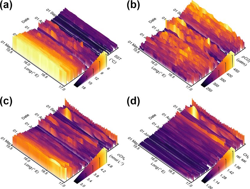
2680                                                  E. Jacobs et al.: Upwelling-induced trace gas dynamics in the Baltic Sea

Figure 1. Map and bathymetry of the study area with typical routes
of SOOP Finnmaid (grey) between Lübeck–Travemünde (L) and
                                                                     Figure 2. Vertical profiles of parameters relevant for this study from
Helsinki (H). Boxes highlight seven regions (solid lines) in which
                                                                     58.58◦ N, 18.23◦ E, on 23 May 2019, which show shapes typical for
we expect upwelling to occur and one in the open Gotland Sea
                                                                     the summer situation in the central Baltic Sea. The profiles display
(dashed lines) as a reference (Table 1). Red dots mark the loca-
                                                                     temperature, salinity, oxygen concentration, CO2 partial pressure,
tions of wind data used for this study, with red arrows indicating
                                                                     and CH4 concentration on an arbitrary scale, truncated at a depth of
upwelling-favourable wind directions. We further marked the is-
                                                                     200 m.
lands of Bornholm (B), Öland (Ö), Gotland (G), Hiiumaa (Hi), and
Utö (U).

                                                                     and Müller, 2018). Pulses of mid-summer bloom events are
and thus upwelling intensity (BACC II Author Team, 2015)             driven by nitrogen fixation (Schneider et al., 2014a); pCO2
and has also been shown to encounter a decrease in oxy-              slightly increases in between due to warming, air–sea ex-
gen at a large number of coastal sites over the last decades         change, and remineralisation of organic matter (Schneider
(Caballero-Alfonso et al., 2015). As a result of these on-           et al., 2014b). Beginning in September/October, deepening
going, strong changes, the Baltic Sea offers the potential to        of the mixed layer leads to increasing pCO2 in the sur-
study feedbacks between anthropogenic and climatic drivers           face water as a consequence of entrainment of deeper wa-
and upwelling-induced greenhouse gas fluxes earlier and              ters that have been subject to organic matter remineralisation
with a higher signal intensity compared to regions that just         (Schneider et al., 2014a). Typical pCO2 values in the cen-
start transforming due to climate change. For instance, “time        tral Baltic Sea range from about 100 to 500 µatm (Schnei-
of emergence” studies suggest that the influence of anthro-          der et al., 2014a), and undersaturation is usually observed
pogenic carbon uptake will not be observable until between           from March/April to September/October, depending on re-
2020 and 2050 in most parts of the global ocean (McKinley            gion (Schneider and Müller, 2018).
et al., 2016).                                                          The methane (CH4 ) distribution in the Baltic Sea is mainly
   The Baltic Sea is characterised by riverine inflow of fresh       governed by the vertical redox and density stratification
water from a large drainage basin and inflows of seawater            (Fig. 2): anoxic, CH4 -enriched bottom water in the deep
from the North Sea, which, together with its basin structure,        basins and CH4 oxidation in the water column, especially
results in a permanent vertical salinity and density stratifica-     in the redox zone located slightly below the permanent halo-
tion (Feistel et al., 2010). A shallow surface thermocline is        cline (Jakobs et al., 2013), lead to strong vertical gradients
present during summer, and large parts of the Baltic Sea are         and concentrations near atmospheric equilibrium in the sur-
additionally characterised by a permanent halocline, with hy-        face water (Schmale et al., 2010; Jakobs et al., 2013). CH4
poxic or even anoxic water underneath (Fig. 2). The typical          is also produced in the upper, oxic water column (Jakobs
seasonality of surface carbon dioxide (CO2 ) partial pressure        et al., 2014; Schmale et al., 2018), partially by zooplankton
(pCO2 ) in the Baltic Sea features a minimum during spring           (Schmale et al., 2018; Stawiarski et al., 2019). The Baltic Sea
and one or more subsequent minima throughout summer:                 acts as a permanent source of atmospheric CH4 . The highest
the spring bloom starts in March/April with the formation            CH4 emissions to the atmosphere are observed in the Gulf
of the surface thermocline and peaks in mid-May (Schneider           of Finland in winter (Gülzow et al., 2013) and in the shallow

Biogeosciences, 18, 2679–2709, 2021                                                      https://doi.org/10.5194/bg-18-2679-2021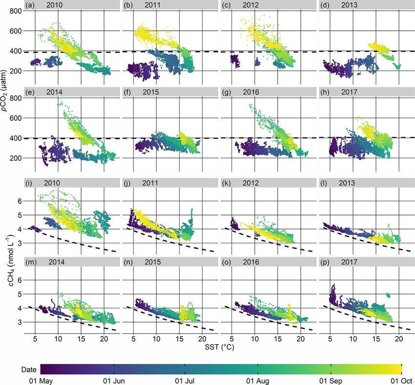
E. Jacobs et al.: Upwelling-induced trace gas dynamics in the Baltic Sea                                                   2681

western basins due to CH4 -rich sediments (Schmale et al.,        for CH4 (e.g. Bange et al., 1994), or cavity-enhanced absorp-
2010).                                                            tion spectroscopy (CEAS; e.g. Gülzow et al., 2011; Du et al.,
   Local coastal upwelling increases both pCO2 and CH4            2014) – a relatively new technique with high sensitivity for
concentration (cCH4 ) in the surface water of the Baltic Sea      both gases (Gagliardi and Loock, 2014). Whereas research
by introducing enriched water from below the summer ther-         cruises enable vertically resolved measurements in a certain
mocline (Fig. 2) to the surface (Gülzow et al., 2013; Nor-        region over several weeks, they do not provide wide tempo-
man et al., 2013; Schneider et al., 2014b; Humborg et al.,        ral and sometimes spatial coverage, which is the main advan-
2019; Stawiarski et al., 2019). However, since previous stud-     tage of autonomous measurements aboard ships of opportu-
ies were limited to episodic events, only little is known         nity (SOOPs). SOOP data sets enable studies with a broader
about the seasonality and regional distribution of upwelling-     perspective that – unlike remote sensing and modelling – are
induced trace gas signals in the Baltic Sea and their re-         still based on in situ measurements. While SOOP-based CO2
laxation. Ferry-based measurements enable studies on up-          measurements are common owing to the available hardware
welling in the Baltic Sea on larger scales, which has already     (Pierrot and Steinhoff, 2019), CH4 measurements are still
been demonstrated for physical parameters in the Gulf of          scarce due to the comparatively recent development of CEAS
Finland (Kikas and Lips, 2016).                                   and the elaborate set-up aboard a SOOP (Gülzow et al., 2011;
   Upwelling events in the Baltic Sea are common but irreg-       Nara et al., 2014). The ferry and SOOP Finnmaid hosts such
ular since they depend on wind conditions (Lehmann and            an autonomous set-up measuring surface concentrations of
Myrberg, 2008). Westerly to south-westerly winds prevail          dissolved CO2 and CH4 since late 2009 using a CEAS sen-
in the Baltic Sea area, which enhances the possibility of         sor (Gülzow et al., 2011), resulting in a unique long-term
upwelling near southern and south-eastern coasts (see red         data set. The vessel transects the Baltic Sea between Lübeck–
arrows in Fig. 1). These upwelling events have a typical          Travemünde (Germany) and Helsinki (Finland) about four
lifetime of several days up to 1 month with sharper hori-         times per week (Fig. 1). SOOP Finnmaid is part of the Ger-
zontal gradients compared to oceanic upwelling (Lehmann           man contribution to the European ICOS (Integrated Carbon
and Myrberg, 2008). In summer, sea surface temperature            Observation System) research infrastructure.
(SST) may decrease by more than 10 ◦ C during an up-                 The large extent to which the Baltic Sea is influenced by
welling event, while salinity changes are usually below 0.5       climatic and anthropogenic forces and the availability of the
(Lehmann and Myrberg, 2008). The influence of upwelling           presented 8-year data set of SOOP Finnmaid and of high-
decreases in autumn and winter, when no seasonal stratifi-        resolution models (Placke et al., 2018; Gräwe et al., 2019)
cation is present. While for oceanic upwelling regions, it is     make the Baltic Sea a unique study site to detect feedbacks
known that upwelling may trigger extreme primary produc-          early and to develop methods and process understanding that
tion through nutrient transport, the influence of upwelling       can be used to analyse long-term data sets with respect to, for
on primary production in the Baltic Sea is still poorly con-      example, upwelling-induced trace gas dynamics. The SOOP
strained (Lehmann and Myrberg, 2008). However, upwelled           strategy allows us to investigate the influence of coastal up-
waters characterised by low nitrogen/phosphorus ratios have       welling on surface pCO2 and cCH4 in the Baltic Sea on a
been reported to fuel cyanobacteria blooms during nitrogen        large spatial and temporal scale without issues of bad cover-
limitation (Vahtera et al., 2005; Lips et al., 2009; Wasmund      age of seasonality due to (biased) individual research-vessel-
et al., 2012). Yet, time lags of about 3 weeks have been re-      based studies. Furthermore, methods developed here can pos-
ported for this feedback with an initial decline in phytoplank-   sibly be used for the treatise of upwelling in other regions.
ton biomass (Vahtera et al., 2005; Wasmund et al., 2012). As      Depending on their size and on the frequency and magnitude
an explanation for this delay, Wasmund et al. (2012) propose      of upwelling, these may be more important for global trace
that the initialisation of a cyanobacteria bloom requires mix-    gas fluxes and budgets compared to the Baltic Sea, e.g. in the
ing of biomass-rich surface water with phosphate-rich up-         case of the large eastern-boundary upwelling systems. In this
welled water.                                                     study, we
   The quantification of dissolved greenhouse gases like CO2
and CH4 across large spatial and temporal scales is critical        – present a method to identify upwelling events along the
to derive accurate climate projections (Friedlingstein et al.,        SOOP track based on wind and modelled SST data
2019) and helps to understand processes involved in the bio-
geochemical cycling of both gases (Takahashi et al., 2009).         – compare upwelling-induced trace gas dynamics within
The latter also necessitates high spatial and temporal reso-          several regions in the Baltic Sea
lution in environments with strong spatial or temporal gra-
dients (Webb et al., 2016). Traditional research cruises usu-       – examine the relaxation of upwelling events over time
ally involve discrete sampling in the water column and often
continuous surface water measurements using an air–water            – discuss interannual variability within the data set and
equilibrator coupled to nondispersal infrared spectroscopy            highlight the importance of upwelling to understand
for CO2 (e.g. Körtzinger et al., 1996), gas chromatography            CO2 and CH4 dynamics in the Baltic Sea

https://doi.org/10.5194/bg-18-2679-2021                                                  Biogeosciences, 18, 2679–2709, 2021
2682 E. Jacobs et al.: Upwelling-induced trace gas dynamics in the Baltic Sea
– evaluate whether a long-term trend can be inferred from
c Calculated as nearest coast in any direction.
b Due to large distances to surrounding coasts.
a Wind directions in brackets have been considered but were found to have only little influence on data from SOOP Finnmaid.
and minimum (min.). This distance is calculated perpendicular to the upwelling-favourable wind direction and based on an average track.
rectangular (Fig. 1); their upwelling-favourable (upw.-fav.) wind direction; and the distance between the track of SOOP Finnmaid within the box and the coast, given as median (med.)
Table 1. Upwelling areas crossed by SOOP Finnmaid (abbreviated and long name); their boundaries (latitude and longitude), including a specification if the respective box is not
openGo
GoF
Hiiu
Go-NW
Go-SE
Ö-E
Ö-S
Born
Abbreviation
the analysis of this 8-year data set taking into account
the interannual variability, and
– demonstrate the potential of extrapolating trace gas ob-
servations based on modelled SST data
Open Gotland Sea
Gulf of Finland
Close to Hiiumaa
North-west of Gotland
South-east of Gotland
East of Öland
South of Öland
Close to Bornholm
Long name
with the aim of
– assessing the prevalence of upwelling and attributing
observed trace gas signals to upwelling
– revealing regional characteristics
– explaining frequently observed features during and after
57.25–58.25
54.75–55.75
upwelling events with a focus on underlying processes
58.75–59.5
56.5–57.75
56.2–57.5
55.5–56.2
59.25–60
Lat (◦ N)
58–59
– identifying controlling mechanisms of seasonality and
variability, and
– showing ways to estimate air–sea trace gas fluxes on
Long (◦ E)
21.5–22.5
17.8–19.5
16.5–17.5
23–24.5
18–19.5
15.5–17
a broader spatial scale under extremely variable condi-
20–21
14–15
tions, which may be a useful method for other upwelling
areas worldwide.
–
Only south-east of Hanko Peninsula
–
Only north-west of Gotland
Only south-east of Gotland
Only east of Öland
–
–
Specification
We present most of the findings by use of illustrating ex-
amples but provide more information in the Appendix, Sup-
plement, and data set.
2 Data and methods
2.1 Measurements aboard SOOP Finnmaid
SOOP Finnmaid is equipped with a variety of sensors to sur-
vey the surface water of the Baltic Sea between Lübeck–
Travemünde in Germany and Helsinki in Finland (Fig. 1). Pa-
rameters including SST, salinity, pCO2 , and cCH4 are logged Upw.-fav. wind
direction (◦ )
every minute. The data set used for this study refers to the
260 (80)a
225 (45)a
time period from May to September and the regions defined
Noneb
in Table 1 and consists of 482 transects from 2010 to 2017.
235
210
260
75
65
The on-board trace gas measurement system consists of
a Los Gatos Research CH4 and CO2 analyser coupled with
Med. (min.) distance
an air–water equilibrator (Körtzinger et al., 1996), which
is described in detail in Schneider et al. (2014b) and Gül-
to coast (km)
zow et al. (2011, 2013), including details on the following
calculations: the measured variables are the mole fractions
64 (40)c
28 (19)
43 (27)
25 (17)
27 (21)
42 (25)
43 (21)
xCO2 and xCH4 in parts per million, which are corrected
10 (4)
to dry-air values using xH2 O data from the same instru-
ment. These mole fractions are converted into partial pres-
sures using atmospheric pressure data and calculating satura-
tion water vapour pressure following Weiss and Price (1980)
under the assumption of 100 % humidity in the equilibrator
headspace. In literature, CO2 data are usually reported as par-
tial pressure or fugacity, while CH4 data are converted into
concentrations. Accordingly, we report pCO2 and cCH4 ; the
latter was calculated from the partial pressure (pCH4 ) us-
ing Bunsen solubility coefficients determined by Wiesenburg
Biogeosciences, 18, 2679–2709, 2021 https://doi.org/10.5194/bg-18-2679-2021
E. Jacobs et al.: Upwelling-induced trace gas dynamics in the Baltic Sea                                                     2683

and Guinasso (1979). Note that we can handle the concentra-          events that SOOP Finnmaid missed. We found that model-
tion (of CH4 in nmol L−1 ) as a quasi-conservative parame-           derived SST data were more suitable than remote-sensing-
ter with respect to temperature changes in the discussion as         derived SST data, which are subject to, for example, cloud
the influence of temperature on water density is negligible in       coverage.
this case. In contrast, the partial pressure (of CO2 ) in equilib-      We used the SST output of the numerical ocean model
rium with the water phase is temperature-dependent (see also         GETM (General Estuarine Transport Model) for the Baltic
Sect. 3.3). To compensate the effect of water warming from           Sea. The model has a horizontal resolution of 1 nmi and 50
inlet to equilibrator, pCO2 is temperature-corrected follow-         vertical terrain-following levels. The uppermost level has a
ing Takahashi et al. (1993). The data set was not corrected          maximum thickness of 50 cm to properly represent the SST
for equilibrator response times, which especially affect CH4         and ocean–atmosphere fluxes. The model run covers the pe-
measurements due to its poor solubility (Webb et al., 2016),         riod from 1961 to 2019. For a detailed analysis of the model
for reasons detailed in Sect. A2.                                    performance see Placke et al. (2018) and Gräwe et al. (2019).
   We post-calibrated xCO2 and xCH4 using a single-point             For the present run, we restarted the model in 2003 but
calibration to a standard gas at near-atmospheric mole frac-         changed the atmospheric forcing to the operational reanal-
tions. These standard gas measurements were performed au-            ysis data set of the German Weather Service (DWD), with a
tomatically when leaving the harbour to yield a drift cor-           spatial resolution of 7 km and a temporal resolution of 3 h
rection between transects. The measurement system aboard             (Zängl et al., 2015). The same wind data – extracted for
SOOP Finnmaid also includes a LI-COR 6262 CO2 and H2 O               one location per upwelling region, respectively (Fig. 1) –
analyser with a separate equilibrator. Even though these addi-       were used to identify upwelling events (Sect. 2.3). To give
tional CO2 data are not presented here, they provided cross-         an impression of the model performance, Fig. 3 and Anima-
validation and quality control. Presenting both CO2 and CH4          tion S1 in the Supplement illustrate SST in the Baltic Sea
measurements from the same instrument ensures the best               during a strong upwelling event taken from both the model
consistency between the two trace gases. Therefore, minor            and a multi-sensor level 3 SST remote sensing product for the
deviations from the previously published CO2 data set in SO-         European seas (Copernicus, 2020). This comparison demon-
CAT (Surface Ocean CO2 Atlas; https://www.socat.info, last           strates both good agreement and the advantage of model data
access: 31 August 2020, Bakker et al., 2016) exist, which is         due to insensitivity to cloud coverage. Differences between
a combined product of both set-ups. In the study area and pe-        modelled SST data along the track of SOOP Finnmaid and
riod, these differences in pCO2 have a median of 0.75 µatm           shipboard SST observations in the entire study area and pe-
and an interquartile range (IQR) of 2.1 µatm.                        riod have a median of 0.04 ◦ C and an IQR of 1.41 ◦ C. Dif-
   We further used monthly averaged atmospheric CO2 and              ferences between model and observations partly result from
CH4 data to calculate atmospheric-equilibrium conditions.            different timescales, i.e. daily means (model data) vs. real
For the closest distance to observations from SOOP Finn-             time (in situ data).
maid, we utilised atmospheric data from Utö station (Finnish
Meteorological Institute, Helsinki) starting in March 2012.          2.3   Identification of upwelling events
Prior to that or to fill gaps in the Utö series, atmospheric
data from Mace Head station (National University of Ire-             Based on the statistical analysis of upwelling in the Baltic
land, Galway) via the NOAA Earth System Research Labo-               Sea by Lehmann et al. (2012), we defined major upwelling
ratories (ESRL) carbon cycle cooperative global air sampling         areas that SOOP Finnmaid crosses (Fig. 1 and Table 1). We
network (Dlugokencky et al., 2019a, b) were used, and both           excluded the Arkona Basin and the Mecklenburg Bight (ar-
data sets were matched to those of Utö by linear regression          eas west of 14◦ E) because strong wind may trigger vertical
(Fig. A2 for details). The atmospheric data are displayed as         mixing through the entire water column in these shallower
atmospheric partial pressure for CO2 or as equilibrium con-          areas, thereby eliminating the usual decoupling between sed-
centration calculated from SST and salinity for CH4 . We also        iment and surface water and greatly enhancing surface trace
plotted relative CH4 saturation, which is the ratio of cCH4 to       gas concentrations (Gülzow et al., 2013). Thus, it is impossi-
equilibrium concentration.                                           ble to disentangle the influence of wind-induced upwelling
                                                                     in these areas by the method proposed here. We included
2.2   Wind and modelled SST data                                     an area in the open Gotland Sea, which should not be di-
                                                                     rectly influenced by upwelling due to being far from the coast
Wind-induced upwelling in summer results in decreasing               (> 40 km; Table 1), for comparison. Furthermore, we only
SST. Thus, to attribute trace gas signals in the data set of         considered data from May to September each year, when
SOOP Finnmaid to upwelling and to assess the spatial and             upwelling-induced SST signals can be observed (Lehmann
temporal dimensions of upwelling events, we combined re-             et al., 2012), which is – together with a wind criterion – the
analysed wind and modelled SST data to locate upwelling              basis of the detection method we used.
events in space and time before starting the actual in situ data        According to Lehmann et al. (2012), we defined an up-
analysis. Using modelled SST data enabled us to also identify        welling event as upwelling-favourable wind, i.e. the wind

https://doi.org/10.5194/bg-18-2679-2021                                                    Biogeosciences, 18, 2679–2709, 2021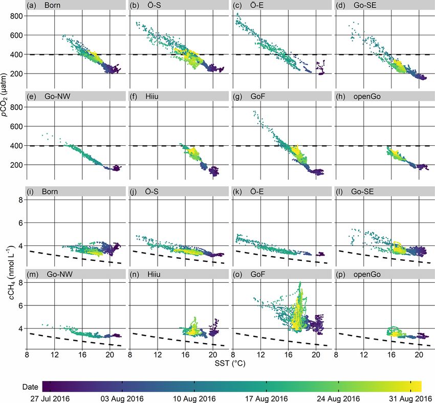
2684 E. Jacobs et al.: Upwelling-induced trace gas dynamics in the Baltic Sea
a more robust median, the boxes were selected to extend be-
yond the actual upwelling areas. This results in a pronounced
increase in 1SST during upwelling events, while the crite-
rion is mostly below the 2 ◦ C threshold otherwise. This cal-
culation can be based first on the entire area inside the boxes
(Fig. A3) or second on just the sub-transects, i.e along the
track of SOOP Finnmaid (Fig. 4). We mainly used the latter
for the purposes of this study, which is justified by a compar-
ison of the capability of both approaches to match a daily
1SST criterion calculated from SST observations aboard
SOOP Finnmaid: the second approach based on sub-transects
is less sensitive (hit rate: 0.57 vs. 0.94 for the first approach)
but has a higher specificity (false alarm rate: 0.08 vs. 0.48)
and better skill to forecast correctly (proportion correct: 0.88
vs. 0.57; critical success index: 0.36 vs. 0.21). These veri-
fication measures were calculated according to Jolliffe and
Stephenson (2003). The differences in number of events cor-
rectly identified depending on which subset of SST data is
used are explained by the fact that upwelling events start near
the coast and then propagate seawards, and thus SST drops
along the sub-transect are delayed and often smaller. The first
approach (using all SST data within the upwelling box) does
not incorporate this lag but is usually better aligned with the
wind criterion for the same reason. Therefore, the appropriate
method choice depends on the desired use: including more
spatial coverage of SST data would be appropriate to analyse
the occurrence of upwelling in a certain region statistically.
However, we chose to use only SST data along the SOOP
route to amplify the agreement with the in situ SST and trace
gas measurements. We provide a more detailed method as-
sessment in Sect. 3.1.
Figure 3. SST in the Baltic Sea on 16 August 2016 (daily mean)
Note that a large-scale upwelling event triggers a drop in
as extracted from (a) the model and (b) the remote sensing prod-
median SST, but due to increased spatial variability during
uct (see text). SST measurements aboard SOOP Finnmaid from the
same day are plotted on top of both panels. We chose this day for those events, the sensitivity of 1SST is usually still sufficient
demonstration purposes as a best compromise between remote sens- to exceed the threshold of 2 ◦ C in these cases (e.g. Figs. 4 and
ing and SOOP data coverage as well as observable upwelling sig- A3 on ca. 10 August 2016).
nals. Animation S1 contains an animation over time with the same
colour scale.
3 Results and discussion
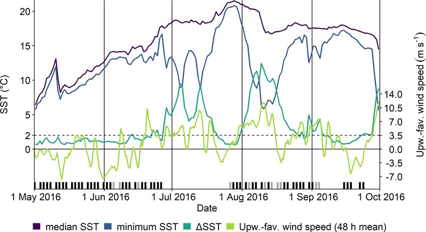
component projected parallel to the coast (Fig. 1) exceeding 3.1 Upwelling statistics based on wind and modelled
3.5 m s−1 for 2 d, causing a temperature drop by more than SST data
2 ◦ C in the respective box. Both criteria (wind and 1SST)
were evaluated per day and box and visualised in yearly To assess the prevalence of upwelling in the data set of
plots, which also display data coverage of SOOP Finnmaid SOOP Finnmaid, we identified the main upwelling periods
(Fig. 4, A3, and A4). and areas along the transect using the method of combining
We calculated the wind criterion as a running mean of a 1SST and a wind criterion (Sect. 2.3). Here, we present
upwelling-favourable wind speeds of the last 48 h with a a summary of the climatological mean number of days per
temporal resolution of 3 h. The criterion is considered to be month and box where the criteria were met (Fig. 5). The
“met” if at least four of the eight mean values per day exceed 1SST criterion was calculated based on sub-transects. We
the threshold of 3.5 m s−1 . provide a full overview further distinguishing by year and
The 1SST criterion was calculated as the difference be- selection of SST data (entire box vs. sub-transect) in the Ap-
tween median and minimum model SST in the respective pendix (Figs. B1, B2, and B3). The wind criterion is usu-
area since a local upwelling event will lower the minimum ally met more frequently than the 1SST criterion calculated
SST, while the median remains relatively stable. To achieve along sub-transects. This reflects that not every occurrence
Biogeosciences, 18, 2679–2709, 2021 https://doi.org/10.5194/bg-18-2679-2021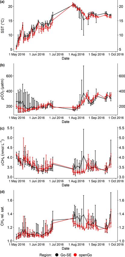
E. Jacobs et al.: Upwelling-induced trace gas dynamics in the Baltic Sea                                                               2685

Figure 4. Time series to demonstrate upwelling detection within the Go-SE box. Purple and blue lines are median and minimum model
SST along the transect of SOOP Finnmaid; the turquoise line shows their difference (1SST). The green line represents the running mean of
upwelling-favourable wind speeds, calculated every 3 h for the last 48 h, respectively. The dashed black line indicates the chosen thresholds
of the 1SST and wind criteria, respectively (2 ◦ C, 3.5 m s−1 ). Each passage of SOOP Finnmaid through the box is marked with a black dash
at the bottom. Grey dashes mark when the ship took the western route around Gotland, thereby missing this particular box on the east side.
A strong upwelling event in August is observed with small data gaps due to SOOP Finnmaid taking the western route. Another event in July
is missed because of a sensor malfunction.

of wind strong enough to induce upwelling leads to upwelled              ever, both criteria are almost never met at the same time,
water masses actually reaching the track of SOOP Finnmaid.               which indicates that the distance between sub-transect and
This is illustrated in Fig. 4 (June 2016) and Animation S1.              coast is too large to observe strong upwelling signals (min-
Downwelling may also lead to quickly vanishing signals                   imum of 27 km, median of 43 km; Table 1). Admittedly, the
(Sect. 3.3). In general, the 1SST criterion is not very sensi-           sub-transect in the Ö-S box is comparable to Hiiu in terms of
tive in May due to a less pronounced thermocline compared                distance to the coast, but the crucial difference seems to be
to summer. Similarly, only small upwelling-induced trace gas             the upwelling-favourable wind direction since strong west-
signals are observed in May, which become greater in late                erly winds are more frequent and intense. This is supported
summer owing to longer decoupling of surface water and                   by the fact that, even if we calculate 1SST based on the en-
underlying sub-thermocline waters (Sect. 3.4). Upwelling in              tire area, the number of days where both criteria are met in
autumn and winter either leads to a general deepening of the             the Ö-S box is higher than in the Hiiu box (Fig. B3), clearly
mixed-layer depth (discussed in Gülzow et al., 2013) or plays            indicating that upwelling is more common in Ö-S. In con-
no important role when the physical and biogeochemical dif-              trast, the sub-transect in the Go-NW box is frequently in-
ferences between surface and upwelled waters have vanished               fluenced by upwelling, but yet, it is the only box where the
in winter.                                                               1SST is met more often than the wind criterion (Fig. 5e). We
   The 1SST criterion based on the entire area is more sen-              attribute this to the small distance to the coast (minimum of
sitive than that calculated along sub-transects but less spe-            4 km, median of 10 km; Table 1) leading to higher SST vari-
cific regarding the prediction of upwelling in dynamic ar-               ability and thus more similarity to the 1SST criterion that
eas like the GoF since it is essentially a measure for SST               includes the entire area (Fig. B3e).
variability > 2 ◦ C within the box (Sect. 2.3). It is triggered              Based on this statistical analysis, we chose the Ö-S box as
more frequently than the wind criterion, and due to the high             an example area for most of the following discussion since
sensitivity of 1SST, the agreement with the wind criterion –             it features prominent upwelling signals concerning both fre-
thus both criteria being met – is high (Fig. B3).                        quency and magnitude. Additionally, data coverage in this
   The Born, Ö-S, Ö-E, Go-SE, and GoF boxes follow sim-                  area is high as it is crossed by SOOP Finnmaid on either of
ilar patterns with respect to both criteria (Fig. 5), which is           its routes (Fig. 1).
not surprising given the fact that in all of these cases, up-
welling is induced by the same south-westerly to westerly                3.2   Regional comparison of upwelling events
winds, and the minimum distances to the coast are rather
similar. The upwelling-favourable wind direction is oppo-                In this section, we investigate upwelling events that were
site in the Go-NW and Hiiu boxes. In the Hiiu box, how-                  caused by strong winds across the entire study area in Au-

https://doi.org/10.5194/bg-18-2679-2021                                                           Biogeosciences, 18, 2679–2709, 2021
2686 E. Jacobs et al.: Upwelling-induced trace gas dynamics in the Baltic Sea
Figure 5. Overview of the two upwelling criteria used in this study: wind (purple) and 1SST (blue). Displayed is the number of days per
month and box in which the respective criterion is met, averaged over 2010 to 2017. 1SST was calculated along the route of SOOP Finnmaid
through the boxes (Sect. 2.3; second approach) to display events that are actually observable from the ship. “Wind + 1SST” (green) only
applies to instances of both criteria being met on the exact same day and therefore excludes occasional instances of lag between wind and
1SST signals. The openGo box is not included here since no upwelling-favourable wind direction can be defined.
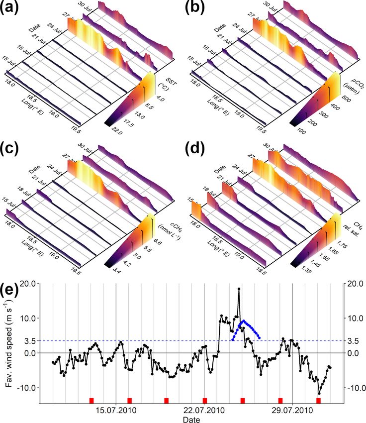
gust 2016, leading to temperature and trace gas signals in The observed trace gas patterns are similar to the temper-
almost all previously defined upwelling areas (Figs. B1 and ature distribution: the first sub-transect can be considered to
B2), which allows us to compare the observations in these be background conditions with typical late summer values
regions and to assess the importance of upwelling for the ob- of about 250 µatm for pCO2 and 3.2 nmol L−1 for cCH4 in
served trace gas dynamics. This case study exemplifies more this area. During the upwelling event, we observe elevated
general findings we gained during the analysis of the entire pCO2 and cCH4 , with trace gas maxima correlated to min-
data set. imum SST. For CO2 , this results in a switch from undersat-
The entire month was characterised by strong westerly to uration to supersaturation. CH4 is always supersaturated or
south-westerly winds (Fig. 4), leading to upwelling in the in equilibrium with the atmosphere in the SOOP Finnmaid
Born, Ö-S, Ö-E, Go-SE, and GoF boxes, interrupted by a data set, and strong upwelling further increases this supersat-
week (15–22 August 2016) of more north-easterly winds, uration and, eventually, CH4 outgassing. However, upwelling
triggering upwelling in the Hiiu and Go-NW boxes. The re- is not the only factor controlling increased CH4 supersatura-
sulting SST drops by up to 16 ◦ C predominantly near all tion (Fig. 6d). Warming of upwelled waters increases pCH4
southern and eastern coasts propagated seawards and relaxed and, therefore, relative saturation. As with SST, the enhanced
within several weeks (Animation S1). Coverage of data from trace gas levels relax subsequentially.
SOOP Finnmaid in this period is very dense, with the ma- To extend these findings to the different regions, we inves-
jority of transects along the east side of Gotland (see ratio of tigated the relationships between trace gas data and temper-
black and grey dashes in Fig. 4). We illustrate the temporal ature over time (Fig. 7). The example from the Ö-S box is
and spatial evolution of this event (Fig. 6) taking the example representative of the majority of strong upwelling events af-
of the Ö-S box. fecting trace gases in the data set of SOOP Finnmaid, which
Before the event, SST is at a typical summer value of 21 ◦ C are generally characterised by near-linear relationships be-
throughout the entire sub-transect. As expected, upwelling tween trace gases and SST. Maximum pCO2 and cCH4
leads to SST decreases (displayed as peaks in Fig. 6a) with values would not be reached without upwelling in summer
temperatures down to 9 ◦ C. These minima move over time (Fig. B4). We observe the same behaviour in the Go-SE, Ö-
(see also Animation S1) and are subject to relaxation, which E, and Go-NW boxes despite their reduced data coverage
is further discussed in Sect. 3.3. The pre-upwelling tempera- (Fig. 7). The Ö-E box features the highest pCO2 in the data
ture is usually not reached again during this time of the year, set of over 800 µatm. In the Go-NW box, the observable up-
most probably due to an increased mixed-layer depth as an welling event began only at the end of trace gas data cover-
additional effect of stronger winds and weakened solar irra- age on the western route due to a different favourable wind
diation at the end of August. direction; hence, the more extreme values are missing in this
example. However, the resulting pattern resembles the ones
Biogeosciences, 18, 2679–2709, 2021 https://doi.org/10.5194/bg-18-2679-2021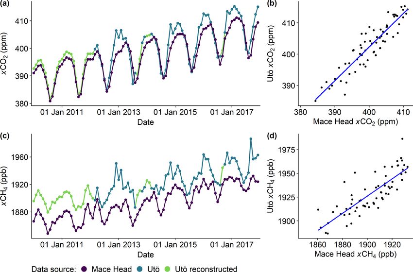
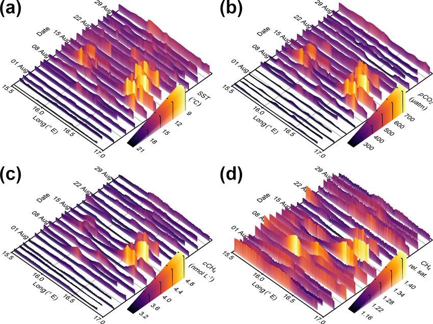
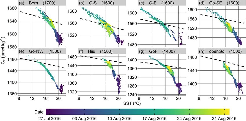
E. Jacobs et al.: Upwelling-induced trace gas dynamics in the Baltic Sea                                                                 2687

Figure 6. (a) Sea surface temperature, (b) CO2 partial pressure, (c) CH4 concentration, and (d) relative CH4 saturation within the Ö-S box
as measured by SOOP Finnmaid on 21 sub-transects from 26 July to 30 August 2016. In all panels, abscissa is position given as longitude,
ordinate is time, and the respective variable is displayed by both colour and height of the curve. Please note the inverted SST scale in (a) to
highlight the correlation between decreasing SST and increasing pCO2 and cCH4 . Data presented in (a–c) correspond to Fig. 7b and j.

of the Ö-S, Ö-E, and Go-SE boxes, just with lower maximum                 we find a clear correlation between decreasing SST and in-
pCO2 and cCH4 .                                                           creasing pCO2 resembling that of the other boxes, we do
   The Born and GoF boxes show the same relationships as                  not observe temperatures lower than 15 ◦ C and pCO2 higher
the previous boxes in their pCO2 –SST diagram, with consid-               than 420 µatm, which is close to atmospheric equilibrium
erable dynamic range in the case of the GoF box (Fig. 7a and              (Fig. 7f). This relationship is similar to that of the openGo
g). The respective cCH4 –SST diagrams, however, only con-                 box, the patterns in which we attribute to mixed-layer deep-
tain a small branch of increasing cCH4 with decreasing SST                ening and air–sea gas exchange caused by stronger winds in-
(Fig. 7i and o). These regions are dominated by temperature-              stead of upwelling because of its distance to the coast (min-
independent CH4 variability, which indicates that other pro-              imum of 40 km, median of 64 km; Table 1). Since the route
cesses than upwelling might cause higher-than-usual cCH4 :                of SOOP Finnmaid within the Hiiu box is the farthest away
the Born box is situated between two basins (Arkona and                   from the coast of all boxes (minimum of 27 km; median of
Bornholm basins), which are interlinked via lateral transport             43 km; Table 1), and the observed pCO2 –SST relationships
and which both feature gassy sediments (Gülzow et al., 2014;              are so similar to openGo, we infer that upwelling has only
Tóth et al., 2014), from which CH4 may be released via pres-              minor influence on the observed values in this region during
sure changes caused by strong winds (Schneider von Deim-                  this time period. This is consistent with maps of modelled
ling et al., 2010; Gülzow et al., 2013); cCH4 variability in the          SST (Fig. 3 and Animation S1; most pronounced around 18
GoF box might be driven by the highly variable physical con-              August 2016), where no upwelled water masses reach out to
ditions, e.g. changes in the estuarine circulation up to full re-         the ship track, and confirms the same finding from the sta-
versal (Westerlund et al., 2019) or enhanced vertical transport           tistical identification of main upwelling areas presented in
by boundary wall shear (Schmale et al., 2010). These effects              Sect. 3.1.
would lead to a less distinct impact of upwelling compared                   The cCH4 –SST diagram of the Hiiu box (Fig. 7n) resem-
to the Ö-S, Ö-E, Go-SE, and Go-NW boxes, where vertical                   bles, to some extent, that of the GoF box (Fig. 7o) without the
decoupling is more stable.                                                upwelling branch and smaller maximum cCH4 and indicates
   The discussed phenomena can be contrasted with the be-                 considerable cCH4 variability compared to, for example, the
haviour of the sub-transect within the Hiiu box: although                 Ö-S, Ö-E, Go-SE, and Go-NW boxes. In late July, for ex-

https://doi.org/10.5194/bg-18-2679-2021                                                            Biogeosciences, 18, 2679–2709, 2021
2688                                                 E. Jacobs et al.: Upwelling-induced trace gas dynamics in the Baltic Sea

Figure 7. Surface pCO2 (a–h) and cCH4 (i–p) as measured by SOOP Finnmaid on 21 transects from 26 July to 30 August 2016, each plotted
against SST within the seven upwelling regions and the open Gotland Sea box for comparison. The measurement date is colour-coded.
Temporal coverage in the Go-SE box (15 transects; see black dashes in Fig. 4) and the Ö-E and Go-NW boxes (6 transects; see grey dashes
therein) is reduced since SOOP Finnmaid uses two different routes around Gotland. Dashed black lines indicate atmospheric-equilibrium
partial pressure for CO2 and concentration for CH4 (calculated using mean salinity per box in the given time period), respectively.

ample, CH4 concentration drops from 4.8 to 3.3 nmol L−1 at            3.3   Typical relaxation of upwelling-induced trace gas
more or less constant temperature (Fig. 7n), equating to a                  signals
change in relative CH4 saturation from 1.9 to 1.3. In the ad-
jacent region of openGo, no instances of increasing cCH4 at           The surface water properties of a region influenced by up-
constant SST (vertical branches in Fig. 7n–p) were observed.          welling change over the course of the upwelling event. This
   We summarise that upwelling affects observed SST,                  can be seen in Fig. 7, where the evolution of the relationship
pCO2 , and cCH4 drastically in the defined boxes in late sum-         over time between SST and pCO2 or cCH4 is indicated by
mer of 2016. It typically causes near-linear relationships be-        colour, and in Fig. B4. Before an event, we observe high tem-
tween surface trace gas signals and temperature with vary-            perature and low trace gas levels, with low spatial variability
ing ranges and slopes between regions. For CO2 , this can             within sub-transects. During strong upwelling, a larger vari-
be observed in all regions (with limitations in the Hiiu box),        ability in SST, pCO2 , and cCH4 is observed concurrently as
while in the case of CH4 , strong variability caused by other         SOOP Finnmaid transects the respective region. Trace gas
processes may mask the effects of upwelling, and closest-to-          and SST data are usually related linearly after the upwelling
linear relationships are observed in the Ö-S, Ö-E, Go-SE, and         event. After upwelling-favourable winds cease, the range of
Go-NW boxes.                                                          signals as well as their intensity is reduced through relax-
                                                                      ation in a quasi-linear fashion (Fig. 7). The final state af-
                                                                      ter relaxation, when compared to the initial state, is shifted
                                                                      towards lower temperatures; higher pCO2 ; and slightly ele-
                                                                      vated cCH4 , which equals a roughly comparable CH4 super-

Biogeosciences, 18, 2679–2709, 2021                                                      https://doi.org/10.5194/bg-18-2679-2021
E. Jacobs et al.: Upwelling-induced trace gas dynamics in the Baltic Sea 2689
The relaxation of SST is mainly driven by mixing. We es-
timated a total surface heat flux of ca. 300 J m−2 s−1 , which
translates to a daily SST change of ca. 0.4 K d−1 assuming a
mixed-layer depth of 15 m, which is rather typical for windy
conditions in summer (derived from model data, not shown).
Therefore, air–sea heat exchange contributes only little to the
observed warming of upwelled water masses on the order of
5–10 K, leaving mixing as the dominant process. Despite the
excess of the surrounding water masses, mixing does not nec-
essarily lead to pre-upwelling conditions since the endmem-
ber may change due to enhanced mixing in the open basins
caused by stronger wind. SST might re-increase in the fol-
lowing weeks depending on meteorological conditions.
Mixing also shapes the typically observed cCH4 –SST re-
lationships (Figs. 7i–o and 8a), leading to near-linear mix-
ing curves since concentration is a conservative parameter
with respect to temperature changes (we neglect the influence
on water density here). The upwelled water mass releases
ca. 7700 nmol m−2 d−1 of CH4 into the atmosphere. This re-
sults in a daily cCH4 loss of 0.51 nmol L−1 d−1 in a 15 m
mixed layer, which is an efficient sink considering the mag-
Figure 8. Theoretical relaxation curves of surface trace gas and
temperature signals caused by upwelling. We calculated all graphs
nitude of observed concentrations. Therefore, air–sea gas ex-
based on the processes (i) air–sea gas exchange, (ii) air–sea heat change alters the slope of the cCH4 –SST relationship. Note,
exchange, and (iii) mixing with a typical water mass with pre- however, that gas flux is highly dependent on wind speeds,
upwelling conditions, with only one process considered at a time, which are biased in cCH4 –SST diagrams presented here: pre-
starting at the point where the three lines intersect. Bold green upwelling conditions involve low wind speeds, while the up-
points highlight the mixing endmembers. Dashed black lines indi- welling event is caused by stronger winds, which eventually
cate atmospheric-equilibrium conditions for the respective trace gas weaken. Heat exchange has no influence on cCH4 , but the
(397 ppm of CO2 , 1920 ppb of CH4 ). Mixing lines were calculated relative CH4 saturation is determined by its partial pressure
for (a) cCH4 using linear interpolation between endmembers (con- pCH4 , which increases by the order of 2 % K−1 (Wiesenburg
servative behaviour), (b) pCH4 from cCH4 and SST, (c) CT using and Guinasso, 1979). This effect should not play a major role
linear interpolation between endmembers whose CT was calculated
concerning relaxation given the low surface heat flux. How-
from AT and pCO2 (conservative behaviour), and (d) pCO2 from
CT and AT . See Sect. B1 for details concerning calculation param-
ever, as outlined above, SST might re-increase in the follow-
eters. ing weeks, thereby increasing pCH4 , and thus potentially
lead to enhanced fluxes into the atmosphere over a longer
time period of weeks following the upwelling event. Like-
wise, mixing leads to elevated pCH4 and relative saturation
saturation at this decreased, final temperature. Depending on compared to linear behaviour (Fig. 8b).
the time of the year, SST might re-increase due to subsequent Similarly, the relaxation of pCO2 cannot be considered in-
warming or not recover completely (as in late summer). dependently from SST relaxation due to its temperature de-
In order to discuss the processes that are involved in pendence. Warming by air–sea heat exchange causes a pCO2
the relaxation of upwelling signals, we calculated theoret- increase on the order of 4 % K−1 (Takahashi et al., 1993),
ical relaxation curves in trace gas–temperature diagrams which should not play a major role concerning relaxation
(Fig. 8). Assumed endmember characteristics, physical driv- given the low surface heat flux. As with pCH4 , however,
ing parameters, and process descriptions are summarised in this effect could lead to increasing pCO2 and enhanced CO2
Sect. B1. We focus on air–sea gas exchange, air–sea heat fluxes into the atmosphere (or reduced fluxes into the sea) in
exchange, and mixing with a typical water mass with pre- the following weeks.
upwelling conditions. CH4 oxidation in the upper, oxic water The relaxation of upwelling-induced pCO2 signals
column should not play a major role on the short timescales (Fig. 7a–g) cannot be explained solely by mixing because
considered here (Jakobs et al., 2013). Primary production the theoretical pCO2 –SST mixing curve obtained from
(e.g. by nitrogen fixation) has the potential to decrease pCO2 CO2 system calculations features a distinct curvature with
distinctly but is difficult to constrain since it depends on me- lower pCO2 compared to linear behaviour (Fig. 8d). The
teorological conditions and nutrient availability with possible observed near-linear relationship is likely caused by air–
time lags of several weeks (Vahtera et al., 2005; Wasmund sea CO2 exchange: at a wind speed of 10 m s−1 , the up-
et al., 2012). welled water mass in this example (Fig. 8d) releases ca.
https://doi.org/10.5194/bg-18-2679-2021 Biogeosciences, 18, 2679–2709, 20212690 E. Jacobs et al.: Upwelling-induced trace gas dynamics in the Baltic Sea 0.074 mol m−2 d−1 of CO2 into the atmosphere, which trans- port out of the box as a possible explanation for this effect lates into a daily CT (total dissolved inorganic carbon) loss based on maps of modelled SST (data not shown). of 4.8 µmol kg−1 d−1 in a 15 m mixed layer. This CT decrease in CO2 -oversaturated waters explains the deviation from the 3.4 Interannual variability in upwelling-induced trace expected linear (conservative) mixing curve in CT estimated gas signals from pCO2 observations (Fig. B5 vs. Fig. 8c). Primary pro- duction triggered by upwelling has a similar (potentially even Since upwelling in the Baltic Sea is an episodic phenomenon greater) influence on pCO2 but with different kinetics. One based on wind conditions, it is subject to considerable inter- could argue that air–sea CO2 exchange should similarly in- annual variability. In Fig. 9, we present seasonal plots (from crease CT in CO2 -undersaturated waters, which is not ob- May to September) of pCO2 and cCH4 versus SST in the served (Fig. B5). This can be explained with the aforemen- Ö-S box. The coloured date scale allows the temporal evolu- tioned wind speed bias, resulting in very low fluxes under tion of signals to be followed throughout the season and also pre-upwelling conditions (see also Sect. 3.5). The bent CT – highlights larger data gaps (e.g. in 2012 and 2013). SST curve translates into a near-linear pCO2 –SST curve, Most years feature consistent patterns with respect to which, in conclusion, can be interpreted as the combined re- pCO2 (Fig. 9), reflecting its yearly cycle (see Introduction sult of mixing and decrease in the highest pCO2 values due and Schneider and Müller, 2018): CO2 is already undersat- to gas exchange and possibly primary production. urated with respect to the atmosphere in May due to pri- The importance of air–sea gas exchange as a relaxation mary production during the spring bloom. Over the fol- process and the potential long-term effect of increasing su- lowing weeks, the change in pCO2 is usually rather small, persaturation due to heat exchange imply that upwelling am- but SST increases as a result of solar irradiation and often plifies surface trace gas fluxes, especially for CH4 , by cir- weaker winds (see also Fig. B4). The resulting stabilisation cumventing the sink of CH4 oxidation in the water column. of the surface thermocline and the accumulation of reminer- Schneider et al. (2014b) mentioned these upwelling-induced alised CO2 below combined with decreasing air–sea CO2 ex- trace gas fluxes previously for the Baltic Sea but questioned change and ongoing primary production lead to increasing the importance for the annual balance since the upper wa- pCO2 gradients between surface and sub-thermocline wa- ter column would be ventilated in autumn and winter any- ter (which are the cause of upwelling-induced pCO2 signals; how, and CH4 turnover times in the upper, oxic water column Fig. 2) and a permanent undersaturation of the surface wa- are on the magnitude of years (Jakobs et al., 2013). Despite ter with respect to the atmosphere. The characteristic cCH4 – a more detailed analysis of the statistical prevalence of up- SST conditions follow the CH4 equilibrium curve towards welling in this study, the question of the importance of up- lower concentrations at higher temperatures most probably welling in the annual trace gas balance of the Baltic Sea can- due to air–sea CH4 exchange, maintaining a persistent super- not be answered here based on the data available. Apart from saturation. In most years, most notably in 2010, 2012, 2014, the high variability within observed upwelling events, gen- and 2016, strong upwelling around August overrides these eral statements on this matter are further complicated by lit- typical summer conditions, resulting in characteristic pCO2 – tle knowledge about fluxes in shallow areas (Humborg et al., SST and cCH4 –SST patterns. For these years, the ranges of 2019), large heterogeneities between basins (Gülzow et al., SST, pCO2 , and to a certain extent cCH4 are similar (but still 2013), and the unknown CO2 source and sink behaviour of not equal), with the notable exception of very dynamic cCH4 the entire Baltic Sea (Schneider et al., 2014b). Answering in 2010. For the other years, we observe a high degree of this question in the future requires more knowledge of the variability from these typical conditions: strong upwelling- Baltic Sea CO2 and CH4 balances in general and extended favourable winds in June 2011 led to an early increase in insight into limitations of upwelling-induced flux estimates pCO2 and lower SST overall. Later, at the end of July 2011, in the Baltic Sea (discussed in Sect. 3.5). a pronounced, sharp increase in cCH4 at a rather constant Another possible relaxation pathway is downwelling. Fig- temperature was observed, which clearly is not related to up- ure B6 provides an example of quickly vanishing upwelling welling. signals after turning wind. There, we expect downwelling to The year 2015 is particularly interesting because it quickly remove upwelled waters from the surface, thereby demonstrates the influence of quasi-continuous upwelling- restoring the previous surface water mass that underwent favourable winds over the course of several months, which only small changes in SST, pCO2 , and cCH4 . This limits overrides the typical summer trace gas situation. The year enhanced trace gas fluxes to a short time period during the was dominated by upwelling-favourable, westerly winds un- upwelling event. This example is rather unique because it re- til the beginning of August (Fig. A4), effectively prohibiting quires upwelling- and downwelling-favourable wind condi- strong thermal stratification of the surface water (Fig. 10a tions in quick succession and can only be observed in close and low maximum temperature in Fig. 9f and n). This spe- proximity to the coast (the Go-NW box in this example), i.e. cial case is problematic for the detection method because where the upwelled water mass is young and has not yet ex- the observable 1SST gradients become too small for every panded towards the open sea. We can exclude lateral trans- day to be counted as an “upwelling day” (Fig. A4). As a Biogeosciences, 18, 2679–2709, 2021 https://doi.org/10.5194/bg-18-2679-2021
E. Jacobs et al.: Upwelling-induced trace gas dynamics in the Baltic Sea                                                             2691

Figure 9. Surface CO2 partial pressure (a–h) and CH4 concentration (i–p) from 1 May to 30 September within the Ö-S box, each plotted
against temperature for individual years. The measurement date is colour-coded. Dashed black lines indicate atmospheric-equilibrium partial
pressure and concentration (calculated using mean seasonal salinity), respectively.

result of weakened stratification, surface CO2 undersatura-                It was not possible to identify trends in frequency or mag-
tion is unusually weak compared to the typical summer sit-              nitude of enhanced pCO2 and cCH4 caused by upwelling
uation (Fig. 10b and high minimum pCO2 in Fig. 9f). Fur-                events on the limited timescale of 8 years covered by our ob-
thermore, we observe reduced cCH4 variability as a result of            servations. The main reason for this is the high spatial and
continuous mixing and intensified air–sea exchange through              temporal variability in upwelling (and of several other pro-
increased turbulence so that cCH4 follows the equilibrium               cesses with influence on dissolved trace gases) in the Baltic
curve more closely than during most years (Fig. 9n). Ele-               Sea, which led to the necessity to do parts of the analyses on a
vated cCH4 (Fig. 10c) does not necessarily translate into el-           per-event basis and effectively impeded a universal approach.
evated saturation (Fig. 10d) depending on SST; however, as              Moreover, the observed endmembers of minimum SST and
pointed out in Sect. 3.3, the water mass will become super-             maximum pCO2 and cCH4 are dependent on data coverage,
saturated as a consequence of subsequent warming. In July               which adds another layer of uncertainty to any trend analy-
2015 (turquoise hues in Fig. 9f and n), near-linear trace gas–          sis on the data set, especially in boxes around Gotland (two
temperature curves are characteristic for strong upwelling              different ship routes) and during years with larger data gaps.
(see Sect. 3.2). Compared to, for example, August 2014 and              Typical water residence times of 10–30 years (Feistel et al.,
2016, however, where the upwelling SST, pCO2 , and cCH4                 2010) imply that longer trace gas time series are needed to
signals stand out prominently from the rest of the values,              detect not only variability but also trends using the meth-
their range concerning all three parameters is reduced in               ods we presented here. In fact, Schneider and Müller (2018)
2015 since decoupling of surface and underlying water was               managed to find a trend in surface pCO2 between 4.6 and
partly impeded.                                                         6.1 µatm yr−1 in the Baltic Sea from 2008 to 2015 but did
                                                                        so without a focus on upwelling events only and by filling

https://doi.org/10.5194/bg-18-2679-2021                                                         Biogeosciences, 18, 2679–2709, 2021
You can also read