A functional connectivity atlas of C. elegans measured by neural activation - arXiv
←
→
Page content transcription
If your browser does not render page correctly, please read the page content below

A functional connectivity atlas of C. elegans
                                           measured by neural activation
                                           Francesco Randi1 , Anuj K Sharma1 , Sophie Dvali1 , and Andrew M Leifer1,2,*
                                           1 Princeton University, Department of Physics, Princeton, NJ, 08544, United States of America
                                           2 Princeton  University, Princeton Neurosciences Institute, Princeton, NJ, 08544, United States of America
                                           * leifer@princeton.edu
arXiv:2208.04790v1 [q-bio.NC] 9 Aug 2022

                                           ABSTRACT

                                           Neural processing and dynamics are governed by the details of how neural signals propagate from one neuron to the next
                                           through the brain. We systematically measured functional properties of neural connections in the head of the nematode
                                           Caenorhabditis elegans by direct optogenetic activation and simultaneous calcium imaging of 10,438 neuron pairs. By
                                           measuring responses to neural activation, we extracted the strength, sign, temporal properties, and direction of information flow
                                           between neurons in order to create an atlas of causal functional connectivity. We find that functional connectivity differs from
                                           predictions based on anatomy, in part, because of extrasynaptic signaling. Our measurements show that neurons such as RID
                                           signal extrasynaptically to other neurons for which there are no direct wired connections. We show that functional connectivity
                                           better predicts spontaneous activity than anatomy, suggesting that functional connectivity captures properties of the network
                                           that are critical for interpreting neural function.

                                           Main
                                           Introduction
                                           Brain connectivity mapping is motivated by the claim that “nothing defines the function of a neuron more faithfully than the
                                           nature of its inputs and outputs”1, 2 . One way to measure inputs and outputs is to make a map of the anatomical electrical
                                           and chemical synapses of a brain, called a connectome. The connectome of the nematode C. elegans3–5 has informed our
                                           understanding of circuit-level mechanisms underlying mechanosensation6 , locomotion7 , chemosensation8 , and other behaviors
                                           and also serves as the basis for connectome-constrained models of neural activity9, 10 . Connectomes for Ciona intestinalis
                                           larvae11 , Drosophila larvae12 , larval zebrafish13 , and adult Drosophila14, 15 are at various stages of completion, and have already
                                           elucidated circuit-level mechanisms, such as those underlying the head-direction system in the adult fly16, 17 . Efforts to measure
                                           the mouse connectome are also underway18 .
                                               Yet, an anatomical map of synaptic contacts leaves ambiguous some aspects of neurons’ inputs and outputs. One cannot
                                           always infer a neural connection’s strength and sign (excitatory or inhibitory) from anatomy or gene expression. For example,
                                           the strength and sign of the C. elegans synapses from neurons ASE to AIB are ambiguous because ASE releases glutamate
                                           and AIB expresses both excitatory and inhibitory glutamate receptors19 . Anatomy does not provide a clear picture of the
                                           timescales of neural transmission because these timescales are governed by molecular properties that are hidden from view.
                                           Moreover, not all anatomical neural connections are operational. In the head compass circuit in Drosophila, many anatomical
                                           connections exist, but plasticity from long-term potentiation and long-term depression selects only a subset to function in
                                           order to guide relevant visual inputs20 . Similarly functional connections in the central complex appear to be sparser than
                                           expected from anatomy21 . Neuromodulators also adjust the properties of neural connections to strengthen or weaken them or to
                                           turn on only a subset of circuits out of a larger menu of possible latent circuits, for example, in the stomatogastric ganglion
                                           (STG)22–24 . Additionally, neurons can release many signaling molecules from outside the synapses, to facilitate “wireless”
                                           neural connections that are not visible in the anatomical wiring25 , as we explore in this work. These additional properties of a
                                           neuron’s inputs and outputs pose challenges for accurately predicting a network’s activity or function from anatomy alone.
                                               A more direct way to characterize the nature of a neuron’s inputs and outputs is to measure their functional properties
                                           directly, namely by activating a neuron and observing responses in other neurons. We refer to this approach as “measuring
                                           functional connectivity,” because our measurements are used to define mathematical functions that describe how neural signals
                                           of an upstream neuron drive activity in a downstream neuron. The general approach of activating a neuron and measuring a
                                           response has also been described as “influence mapping”26 . Functional connectivity measured by neural activation captures
                                           the strength and sign of neural connections and reflects plasticity, neuromodulation, and even wireless signaling. Measuring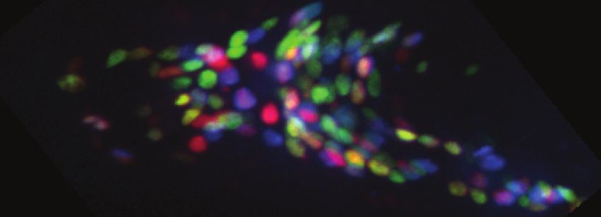
downstream responses to neural activation provides an unambiguous arrow of causality and temporal dynamics, in contrast
to correlative maps of spontaneous activity. Perturbing the network allows us to probe neural connections that might not be
active spontaneously, and therefore would be omitted from a correlation map. Previous efforts have employed optogenetic
perturbations27, 28 and calcium imaging29, 30 in vivo to map the functional connectivity of selected circuits in C. elegans31 ,
mouse visual cortex32 , mouse hippocampus33 , mouse somatosensory cortex34 , and zebrafish35 , among others. More recently,
investigators measured a functional connectivity map of the Drosophila central complex by probing genetically defined cell
types in order to relate functional connectivity to anatomy21 .
    Here we use neural activation to measure functional connectivity of neurons from throughout the head of C. elegans instead
of any specific circuit or brain area. We survey 10,438 neuron pairs to present a systematic functional connectivity atlas of
neural connections in the head. We show that functional measurements are more suitable for predicting spontaneous activity
than anatomy and gene expression, and that the functional description captures instances of wireless signaling that are absent
from anatomy.

Simultaneous population imaging and single-cell activation
To probe functional connectivity, we systematically activated each neuron, one at a time, while simultaneously recording
network activity. We recorded population calcium activity from 43 wild-type (WT) background animals, each one for up
to 40 min, while stimulating a randomly selected sequence of neurons one-by-one every 30 s (Fig. 1). To perform these
measurements, we combined whole-brain population calcium imaging via spinning disk single-photon confocal microscopy37, 38
with two-photon39 targeted optogenetic stimulation40 in an immobilized animal (Fig. 1a). Animals are awake and pharyngeal
pumping is visible during recordings. We spatially restricted the optogenetic excitation volume in three dimensions to the typical
size of a C. elegans cell soma (Supplementary Fig. S1a) using temporal focusing33, 41 to address a single neuron without also
activating its neighbors (Supplementary Figs. S2 and S3). To overcome challenges associated with spectral overlap33, 34, 42–44 ,
we expressed the GUR-3/PRDX-2 purple-light activatable optogenetic system45, 46 and a nuclear-localized calcium indicator
GCaMP6s47 in each neuron (Fig. 1b). For calcium imaging, we used a wavelength and intensity of excitation light that does
not elicit photoactivation of GUR-3/PRDX-2 (Supplementary Fig. S1b)48 . We also included additional genetically encoded
fluorophores from NeuroPAL36 to identify neurons consistently across animals (Fig. 1c). Many neurons exhibited calcium
activity in response to activation of one or more other neurons (Fig. 1d). A downstream neuron’s response to a stimulated
neuron is evidence of a functional connection between them.
    We highlight three examples of excitatory or inhibitory responses that we observed among interneurons in the motor
circuit (Fig. 1e-g). Stimulation of the interneuron AVJR evoked activity in AVDR (Fig. 1e). AVJ is thought to coordinate
locomotory activity upon egg laying and has been proposed to promote forward locomotion49 . AVD activity is associated with
sensory-evoked (but not spontaneous) backward locomotion6, 7, 50, 51 and receives chemical and electrical synaptic input from
AVJ5, 52 . Both the wiring and our functional measurements suggest that AVJ may also play a role in coordinating backward
locomotion, in addition to its previously described roles related to egg laying and forward locomotion.
    The premotor interneurons AVA31, 51, 53–58 and AVE51, 55 both exhibit increased calcium activity during backward movement
that is correlated with one another55 . AVE has gap junctions and makes many chemical synaptic contacts with AVA5, 52 . We
found that stimulating AVE evoked activity in AVA (Fig. 1f). In contrast, stimulation of AVE inhibited activity in SAAD
(Fig. 1g). SAAD is involved in turning behavior and has been proposed to inhibit motor neurons associated with backward
locomotion in order to prevent conflict between turning and reversal circuitry51 . Our measurements suggest a complementary
mechanism in which the backward-associated AVE neuron functionally inhibits the turning machinery via inhibition of SAAD.

Activation-response map
We generated a single activation-response map by aggregating downstream responses to stimulation for each neuron pair across
recordings from 43 individuals (Fig. 2). We report the average calcium response in a time window h∆F/F0 it averaged across
trials and animals (Supplementary Fig. S4). We imaged calcium activity in response to stimulation for 10,438 neuron pairs (30
% of all possible pairs in the head) at least once, and as many as 27 times (Supplementary Fig. S5a). This includes activity from
162 of 188 neurons in the head (86 %, Supplementary Fig. S6). To assess the significance of the average observed calcium
transients in each neuron pair, we compared features of the transients to a null distribution of activity recorded from animals
in which no neurons had been stimulated. We then accounted for multiple hypotheses and calculated a q-value for each pair
that reports significance59, 60 considering both the magnitude of the response and the number of observations (Supplementary
Fig. S5b). Our activation-response map comprises the response amplitude and its associated q-value (Fig. 2a, Supplementary
Fig. S7).
     This functional dataset, overlaid on the anatomical wiring diagram5, 52 , is browseable through online interactive visualization
software (https://funconn.princeton.edu) built on the NemaNode platform5 . If we hold the false discovery rate at
5% (q < 0.05), we estimate that at least 1,285 of the 10,438 measured neuron pairs in our compiled datasets are functionally
connected, or 12 % (Fig. 2b,c). Note that these functional connections are “effective connections” because they represent

                                                                                                                                2/36
a.             1P Ca2+ Imaging       b.

                                                                                                                  ΔF/F0
                                          Spinning Disk Confocal
                                                                                         GCaMP6s &
                                          Tunable                                        Other Fluor.   GUR-3/PRDX-2 Time
                                          Lenses
                                     2P
                                 Stimulation
                                                                   c.

                                                      *

                               d.
                                       Stim:
            Responding Neuron

                                                                        Time (s)
             e.                                                         f.
                                                                             Sorted Trials

                                                                        g.
                     Sorted Trials

                                                                        Sorted Trials

Figure 1. Measuring causal brain-wide functional connectivity at a cellular resolution. a.) Schematic of instrument
that allows sequential stimulation of individual neurons while population calcium activity is simultaneously recorded. b.) A
spatially restricted two-photon excitation spot activates GUR-3/PRDX-2 during single-photon GCaMP6s calcium imaging. c.)
Additional fluorophores from NeuroPAL36 are expressed to identify neurons. d.) Example recording from an individual worm.
Calcium activity is simultaneously recorded from 74 neurons with unambiguous neural identities. Stimulation events are shown
as gray vertical lines, and the identity of the stimulated neuron is listed at top. For visualization, activity is shown as
fluorescence intensity normalized by noise F/σF . e.) Paired activity of AVJR and AVDR in response to AVJR stimulation is
shown as the fold change of fluorescence from baseline, ∆F/F0 . Top panel shows mean (blue line) and standard deviation (light
shading) across trials and recordings. Bottom panel shows simultaneously recorded paired activity for individual trials,
including across animals, sorted by mean activity in AVDR. All trials with stimulus events that resulted in activity in the
stimulated neuron above a threshold are shown. f.) Same as e for AVER stimulation and AVAR response. g.) Same as e for
AVEL stimulation and SAADL response.
                                                                                                                            3/36
a

                          Sensory
         Responding
                          Interneuron

                                                                                                                                                                             >0.4      0.0
                                                                                                                                                                                  value

                                                                                                                                                                                   No
                                                                                                                                                                                   measurement
                          Motor

                                                        Sensory                                           Interneuron                          Motor
                                                                                            Stimulated
         b
                                                                                                                                       D
                                                                                                                                   A       P                      Sensory
                                                                                                                                       V                          Interneuron
                                                                                                                                                                  Motor

         c                                              d                                                  e                                           f
         Prob of q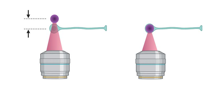
the propagation of signals over all paths in the network between the stimulated and responding neuron, not just the direct
(monosynaptic) connections between them.
    C. elegans neuron subtypes typically consist of two bilaterally symmetric neurons, often connected by gap junctions, that
have similar neural wiring52 , similar gene expression61 , and correlated activity62 . Our measurements show that bilaterally
symmetric neurons are four times more likely to be functionally connected than pairs of neurons chosen at random (Fig. 2c).
    We observe both excitatory and inhibitory calcium responses in the activation-response map. For example, activation of
neuron RIS evokes inhibitory transients in many neurons (Supplementary Fig S8), consistent with its expected role in inducing
quiescence63, 64 . The balance of excitation and inhibition is important for a network’s stability and a lack of balance may lead to
dysfunction65, 66 . In the mammalian cortex, approximately 20% of cells are inhibitory67 and similar values were predicted for
the fraction of synapses in C. elegans based on wiring and gene expression patterns68 , but until now this has not been directly
measured in the worm. Our measurements indicate that 33 % of q < 0.05 functional connections are inhibitory (Fig. 2d),
which suggests that there may be commonalities in the levels of excitation and inhibition across animals and across network
descriptions.
    Neurons with a single-hop anatomical connection were more likely to be functionally connected at q < 0.05 compared
to neurons with only indirect anatomical connections, and the likelihood decreases with increasing minimal anatomical path
length (Fig. 2e). We investigated how far responses to neural stimulation penetrate into the anatomical network. Functionally
connected (q < 0.05) neurons were on average connected by a minimal anatomical path length of 2.3 hops (Fig. 2e), suggesting
that neural perturbations often propagate multiple hops through the anatomical network or that neurons are also signaling
directly through non-wired means, as explored later.
    We observed two types of variability in neural responses for many neuron pairs across trials and individuals: (1) a
downstream neuron responds to stimulation of a given upstream neuron in only some simulations but not others (Fig. S9a)
and (2) the amplitude, temporal shape, and sign of the response can vary across trials or individuals. Some variability in the
responding neuron’s activity can be attributed to variability of the activity in the upstream neuron. For example, in Fig. 1f,
downstream neurons with weak responses occurred when upstream neurons had weak auto-responses to stimulation. (We refer
to a neuron’s response to its own stimulation as an auto-response.) To study variability in the strength, temporal properties, and
sign of the connection, while excluding variability contributed by the upstream neuron’s activity, we calculated a kernel for each
stimulation that caused a response. The kernel gives the activity of the downstream neuron when convolved with the activity of
the upstream neuron. The kernel describes how the signal is transformed from the upstream to the downstream neuron for
that stimulus event, including the timescales of the signal transfer (Supplementary Fig. S10). We characterized variability of
each functional connection by comparing how these kernels transform a standard stimulus (Fig. S9b). Many neuron pairs had
collections of kernels with properties that varied across trials. We did not identify the sources of this variability, but they likely
include state- and history-dependent effects69 , including from neuromodulation22, 70 , habituation and plasticity, and inter-animal
variability in wiring and gene expression. Collections of kernels within a neuron pair were more stereotyped than collections of
kernels randomly selected from across shuffled pairs (Fig. S9c), as expected.

Functional connectivity differs from anatomy
We sought to compare our measured functional connectivity to anatomy5, 52, 71 . Functional connectivity and anatomical
connectivity describe different levels of the network – functional connectivity measures effective connection between two
neurons, including contributions from all paths through the network, direct and indirect (Fig. 3). In contrast, anatomical features
such as synapse count are properties of only direct connections between two neurons. A bridge is needed between these two
levels of description in order to make a like-to-like comparison. Therefore, we used connectome-constrained simulations
to derive properties of effective connections from anatomy. We systematically activated neurons in silico and simulated the
network’s response, using known synaptic weights from anatomy5, 52 , synaptic polarities based on expression of three common
neurotransmitters and receptors68 , and common assumptions about timescales and dynamics72 . We found poor agreement
between those response amplitudes derived from anatomy and those functional measurements in our activation-response map
(Fig. 3b). Our measurements indicate that functional connectivity differs from what one would expect based on anatomy.
    Three hypotheses may explain why functional connectivity disagrees with predictions of neural dynamics derived from
anatomy. The first is that the strength or sign of connections may have been misinterpreted or otherwise insufficiently specified
from anatomy. A second and not mutually exclusive hypothesis is that additional connections exist that are not present in the
anatomical wiring. A third possibility, that we do not explore, is that existing computational models may fail to predict neural
responses even when given accurate strength, sign, and connectivity – e.g., because they rely on incorrect assumptions about the
biophysical dynamics of synapses. Here, we consider the first two hypotheses: (1) incorrect strengths or signs and (2) missing
connections.
    There are known instances in which anatomy leads to incorrect predictions about the functional strength or sign of
connections. For example, the somatosensory neuron AFD’s primary synaptic partner is AIY. The overall functional connection

                                                                                                                                5/36
a.                            b.                                                       c.                                   d.
 Effective Connection

                                                                                                                           anatomy-derived response
                                                                                                                             Fraction agreeing with


  A            Indirect
               Path Indirect

                                                                                         ρ1-q,ΔV
  Direct               Path


   Path
              B

                                                                                                   Head     Head Pharynx                              Fast    Slow
                                                         Anatomy-derived response (V)                      (fitted
                                                                                                          weights)                                       q
between AFD and AIY had at one time been thought to be inhibitory because AFD releases glutamate and AIY expresses
inhibitory metabotropic glutamate receptors. However, our functional measurements (Supplementary Fig. S11) and prior
optogenetic and electrophysiology recordings all show that AFD-AIY is in fact functionally excitatory, likely due to peptidergic
signaling between the two neurons73 . In this case, even if anatomy and gene expression correctly predict network topology and
transmission across the synaptic cleft, there may be other modes of communication such as extrasynaptic peptidergic signaling,
and this might explain why predictions from anatomy disagree with functional measurements.
    To investigate whether strengths or signs had been misinterpreted from anatomy, we tested whether adjusting the strengths
and signs of neural connections could bring anatomical predictions of neural responses into closer agreement with functional
connectivity. We constructed a connectome-constrained model of neural activity in which we allowed the strength and sign
of the direct anatomical connections to be fit in order to best reproduce the measured effective functional connections, while
preserving the overall network topology (i.e., allowing no new connections). For simplicity during fitting, we assumed a linear
network at steady state, but during the comparison we relaxed this assumption and ran full simulations. Even when allowing
the anatomical weights and signs to change in the most favorable way – without adding any new connections – the agreement
between anatomical wiring and our functional connectivity measurements remained poor (Fig. 3c bar laeled “Head, fitted
weights” in ). Our measurements suggest that adjusting anatomical weights and signs alone is insufficient to bring anatomy into
agreement with functional connectivity. We therefore explored the hypothesis that anatomy omits connections that are needed
to accurately predict neural responses.

Wireless signaling
Neurons can communicate extrasynaptically by releasing transmitter via dense core vesicles from areas of the neuron beyond the
synapse that then diffuses through the extracellular milieu to bind to receptors of other neurons. This extrasynaptic communica-
tion, sometimes called volume transmission74 , creates neural connections that are hidden from anatomy. Extrasynaptic signaling
can be mediated by several classes of molecules including GABA75, 76 , NMDA77 , monoamines25 , and neuropeptides78 and
these form an additional wireless layer of communication in the C. elegans nervous system25 . Neuropeptides and neuropeptide
receptors in particular are reported to be ubiquitous across the C. elegans nervous system61 and are one possible substrate for
extrasynaptic communication.
    Extrasynaptic signaling acts in two ways that are not mutually exclusive: (1) they act as neuromodulators to alter excitability
or synaptic properties and change how neurons respond to inputs22, 78 and (2) they alter the activity of neurons themselves.
While the former might appear as variability in our functional connectivity measurements, the latter should appear as neural
responses.
    Two observations hinted that missing anatomical connections in the form of extrasynaptic signaling may partly explain
why our functional connectivity differs from anatomy. First, we noticed that agreement between functional connectivity and
anatomy, while still poor, improved slightly when we considered only those neural connections in the pharyngeal network
(Fig. 3c). Neural connections in the pharynx are less likely to be wireless than neural connections in the rest of the brain.
Specifically, the fraction of functional connections that is thought to be mediated by monoamines and neuropeptides is only
28% in the pharynx but 58% in the head based on anatomy and gene epression5, 25 . Therefore, anatomy may better agree with
our measured functional connectivity in the pharynx because the anatomical description of the pharynx may omit a smaller
proportion of connections.
    Second, fast functional connections showed better agreement with anatomy than did slow functional connections (Fig. 3d.)
Extrasynaptic signaling is expected to be slower than chemical or electrical synapses, because instead of traveling across the
short synaptic cleft, signaling molecules must diffuse further through the extracellular milieu to reach targeted neurons. The
slower-timescale connections that we measure may be extrasynaptic and this would explain why they show poorer agreement
with anatomy. Our measurements from the pharynx and of fast and slow functional connections both suggest that extrasynaptic
signaling in our functional measurements may contribute to discrepancies with anatomy. We therefore chose to more directly
investigate extrasynaptic signaling in our measured functional connectivity using mutant animals.
    We measured an activation-response map in unc-31-mutant animals that have deficiencies in extrasynaptic signaling
(Supplementary Fig. S12, 18 individuals) and compared their functional connectivity to WT animals. This mutant disrupts
dense-core vesicle-mediated signaling because it lacks the UNC-31/CAPS protein involved in dense core vesicle fusion79 but is
not expected to disrupt chemical or electrical synapses. An online interactive map allows users to browse the activation-response
map of this mutant and compare it to WT, https://funconn.princeton.edu. As expected, some neural responses in
the unc-31 mutant background were similar to those in WT, including for example functional connections in a small gap-junction
sub-circuit from the pharynx (Supplementary Fig. S13). If extrasynaptic signaling is present in WT animals, it follows that
animals lacking extrasynaptic signaling should have faster and fewer connections overall. As expected, functional connections
in the unc-31 mutant background were more likely to be fast than in the WT background (Supplementary Fig. S14a), and had a
smaller proportion of high-confidence functional connections (Supplementary Fig. S14b), further suggesting that extrasynaptic

                                                                                                                             7/36
b.                  URXL response to RID
      a.                                                                         WT

                                                                    Sorted

         c.               ADLR response to RID
                                                                  d.                AWBL response to RID
                       WT                                                  WT
           Sorted

                                                                  Sorted

Figure 4. Anatomy omits extrasynaptic signaling from neuron RID. a.) ADL, AWB, and URX are among the neurons
predicted from anatomy to have no response to RID stimulation because there is no strong anatomical path from RID to those
neurons (vertical line at or near 0 volts). Their RID-evoked anatomy-predicted response is shown within the distribution of
anatomy-predicted responses for all neuron pairs, as in Fig. 3b. b-d.) Activity of neurons b.) URXL, c.) ADLR, and d.) AWBL
are shown in response to RID stimulation in WT and mutant backgrounds. Top panel shows the average across all trials and
animals and bottom panel shows individual traces. Here trials are shown even in cases when RID activity was not measured.

                                                                                                                      8/36
signaling is present in WT functional connectivity.
    We sought to investigate specific extrasynaptic connections that exhibit discrepancies between an anatomical and functional
description. We inspected responses to the neuron RID, a neuroendocrine-like cell80 that is thought to predominantly signal to
other neurons extrasynaptically via neuropeptides such as FLP-14, PDF-1, and INS-1761 .
    RID has many potential extrasynaptic signaling partners but only very few and weak outgoing wired connections (Sup-
plementary Fig. S15a,b) making it a good candidate in which to observe extrasynaptic signaling. In our imaging strain,
RID exhibited only dim tagRFP-T expression, which prevented us from consistently recording its own calcium activity. We
nonetheless stimulated RID and observed other neurons’ responses (Supplementary Fig. S16).
    We inspected the activity of three neuron subtypes, URX, ADL, and AWB, that were predicted to have little or no response
to RID stimulation based on anatomy (Fig. 4a) but showed notably strong responses to RID stimulation when measured in WT
background (Fig. 4b-d). Several lines of evidence led us to conclude that RID predominantly sends signals to URX, ADL and
AWB extrasynaptically. (1) When RID was stimulated in the unc-31 background, these three neurons all exhibited reduced
amplitude or were less likely to respond at all, suggesting that these neurons’ connections to RID are dense-core-vesicle-
dependent and likely extrasynaptic. (2) All three neuronal subtypes express receptors for peptides produced by RID (NPR-4
and NPR-11 for FLP-14 and PDFR-1 for PDF-1). And (3) there are no direct connections through the anatomical network
from RID to URX, ADL, or AWB. The shortest paths from RID to each of the neurons show in (Fig. 4b-d) requires two hops
(l = 2) for URXL and AWBL and three hops for ADLR (l = 3) and in each case relies on fragile single-contact synapses
that appear in only one out of the four individual connectomes5 . Taken together, RID is a striking example where functional
measurements capture neural responses that are not predicted from anatomy, due to the lack of information about wireless
signaling in anatomy.

Functional connectivity better predicts spontaneous activity than anatomy
A key motivation for mapping neural networks is to understand how they give rise to neural dynamics. We therefore compared
how well functional and anatomical descriptions of the network predict spontaneous neural activity. We measured the
spontaneous network activity of immobilized worms without any optogenetic activators under bright imaging conditions57 .
Activity correlations derived from functional connectivity were notably more predictive of spontaneous neural activity than
were predictions based on anatomy (Fig. 5). We compared spontaneous activity to anatomy in two ways. First, we compared
the bare anatomical weight, or synapse count between two neurons, to the correlation of their spontaneous activity (Fig. 5a).
Previous reports had shown that the anatomical weight between neurons is a particularly poor predictor of correlations in activity
patterns36, 62 and our measurements further support this conclusion. Comparing anatomical weights to spontaneous activity
correlations, however, likely overstates the discrepancy because synapse counts are properties of only the direct connection
between two neurons, while activity correlations instead are influenced by all possible paths through the network. We therefore
also predicted activity correlations derived from anatomy in a second way – by using the connectome-constrained simulations
from Fig. 3. We drove activity in all neurons in the network in silico and measured correlations from the resulting simulated
activity. These anatomy-derived correlations showed marginally better but still poor agreement with measured spontaneous
activity (Fig. 5b, “All driven”).
    We also predicted network activity from our functional measurements. Functionally-derived correlations better predicted
spontaneous activity than either of the anatomy-based approaches (Fig. 5c). To derive correlations from our measured functional
connectivity we drove all neurons in silico, propagated their activity through our measured kernels, and calculated the correlation
matrix from the resulting activity. An interactive version of the simulations we used to derive activity from measured kernels
is available at https://funsim.princeton.edu. All of the parameters in the equations governing neural dynamics,
including the timescales, weights, signs, and connectivity, are extracted directly from the measurements; specifically, they are
captured by the measured kernels. This is in contrast to simulations constrained only by anatomy, which rely on assumptions
about timescales and dynamics. This difference may contribute to why functional connectivity outperforms anatomy at
predicting spontaneous correlations.
    We sought to further improve our predictions of spontaneous activity by inspecting other assumptions in our simulations.
When we derive activity correlations via simulations we face a choice about which neurons should be driven, corresponding
to our estimate of the neurons that drive spontaneous activity in the network. For the analysis above, we drove activity in all
neurons. However, it may be that only a subset of neurons drives the spontaneous activity observed in our recordings. We
therefore tested whether a more optimal subset of neurons improved predictions of spontnaeous activity. We rank-ordered all
the neurons based on how well their individual in silico stimulation reproduced spontaneous network activity and selected the
set of top-n neurons that collectively had the best agreement when driven. For activity derived from measured kernels, we
found that driving activity in the top 20 neurons in silico generated activity patterns with correlations that more closely matched
those of spontaneous recordings (Fig. 5c, “top-n”).
    We next investigated whether selecting an optimal subset of neurons also improved the predictive performance of the

                                                                                                                             9/36
Agreement to spontaneous
                                                                  a.            b.                         c.
                                        (Pearson’s corr coeff )
                                         activity correlations
ΔF/F0

                                                                                                                  Top-N
               A
        Time
                                                                                                                  Driven
                                                                                     Top-N
                                  B
                                                                                     Driven
                                                                                                                    All
                   ΔF/F0

                                                                                       All
                                                                                                                  Driven
                           Time
                                                                                     Driven

          Spontaneous activity                                     Anatomical   Anatomy-derived
              correlations                                                                                 Functionally-derived
                                                                    weights       correlations                correlations

                                                                       A

                                                                                                   ΔF/F0
                                                                                 A                                A
                                                                                                           Time

                                                                           B
                                                                                       B                                         B

                                                                                                                      ΔF/F0
                                                                                                                              Time

Figure 5. Functional connectivity better predicts spontaneous activity than anatomy. Spontaneous activity correlations
are compared to predictions from anatomy and functional connectivity. In each case, agreement is reported as a Pearson’s
correlation coefficient across neuron pairs. Schematic illustrates the measurements used to predict spontaneous activity
correlations. a.) Anatomical weights from the synapse count are directly compared to the correlation matrix of spontaneous
activity. b.) Correlations in the anatomy-derived activity are compared to correlations of spontaneous activity. A
connectome-constrained simulation is used to derive activity correlations from anatomy by driving neurons in silico. Two
variations of anatomy-derived activity are shown: when all neurons are driven (dark blue) or when only an optimal subset of
top-n neurons is driven (light blue). For anatomy, the optimal set is the set of all neurons so the two bars are the same. c.)
Measured functional connectivity kernels are used to simulate activity. Correlations of functionally-derived activity are
compared to those of spontaneous activity. Agreement to spontaneous activity is shown for two variations of
functionally-derived activity: when all neurons are driven (dark blue) or when only an optimal subset is driven, in this case the
top 20 (light blue).

                                                                                                                                     10/36
anatomy. Unlike for functional connectivity, for anatomy-derived activity we did not find any top-n subset that significantly
improved performance. The best performing set of top-n neurons was the set of all neurons (Fig. 5b, “top-n”). Thus, in all
cases, functionally derived activity outperformed anatomy-derived activity, further indicating that measurements of functional
connectivity are more effective than anatomy at predicting properties of real neural activity.
Discussion
A key finding from this work is that the functional connectivity of C. elegans differs from predictions based on anatomy and
gene expression. Why such a discrepancy? One answer is that anatomy fails to account for wireless connections25 . For example,
we show specific functional connections in which RID signals extrasynaptically via peptides and this type of connection is not
visible in anatomy. This explanation is consistent with recent gene expression profiling results showing that the molecular
machinery for neuropeptide signaling is ubiquitous in the C. elegans nervous system61 . Here, we present evidence that wireless
signaling is present in the functional connectome and provides a meaningful contribution to neural dynamics.
What are the implications of wireless signaling for interpreting connectivity in other organisms? In mammals, hypothalamus
and midbrain exhibit peptidergic signaling and even mouse cortex widely expresses molecular machinery for neuropeptide
signaling81 . Diffusion would appear to place strict limits on the speed, strength, and spatial extent of extrasynaptic signaling in
the brain. Therefore, the small size of the worm’s head (50x50x150 microns) may make it particularly amenable to extrasynaptic
signaling. However, in larger vertebrate brains, signaling molecules may circumvent limits of diffusion by traveling through
the vasculature, as is the case for hormones in the neuroendocrine system. More research is needed to determine the role of
wireless signaling in generating neural dynamics in vertebrates. If studies show that wireless signaling is important, functional
measurements will be needed to complement anatomy for accurately predicting neural dynamics.
Other factors likely also contribute to the discrepancies between the anatomical and functional descriptions of this network.
Researchers have suggested that anatomy may represent a superset of possible connections in the brain, but that only a subset
of connections are active while the rest are dormant, waiting to be activated by either neuromodulators23, 24 (e.g., as in the STG)
or plasticity (e.g., as in the Drosophila head direction circuit)20 . An important future study on functional connectivity will be to
map these latent circuits and determine when they turn on or off.
To map the functional connectivity presented here, we measured activity in response to the stimulation of 133 identified
neurons, corresponding to 71 % of all 188 neurons in the head. We found 1,285 functional connections, with a false discovery
rate of q < 0.05. This result likely underestimates the true number of effective connections for several reasons. Our analysis
omits some neurons visible in our recordings because they are either too dim or too difficult to unambiguously identify, even
with color information provided by NeuroPAL fluorophores. For example, the neuron AVB is consistently very dim, and
identifying neurons in the ventral ganglion is challenging. Other neurons such as RID are bright enough to be stimulated,
but not bright enough to always track and observe calcium responses, and so their functional connections are undercounted
in the maps of Fig. 2. We also do not expect to detect neural responses that lack calcium activity in the nucleus, such as
compartmentalized calcium dynamics82 . More generally, the lack of an observed response does not conclusively indicate that
no functional connection exists. As discussed in21 , because we are limited by the efficiency of stimulation and the sensitivity of
the GCaMP6s reporter, our results may not capture weak or variable effective connections. Future work with voltage indicators
may provide better sensitivity.
Conversely, we are unlikely to overestimate the prevalence of functional connections. We exclude apparent responses
that would have likely arisen without stimulation by comparing response amplitudes to recordings in which no stimulation
was delivered. We also control the false discovery rate in the face of multiple hypothesis testing. Therefore, the functional
connectivity map presented here represents a lower bound on the complete set of functional connections in the worm.
The measured functional connectivity map reports effective connections, not direct connections. Effective connections are
the most relevant and useful for answering the circuit-level questions that motivate our work. These connections describe how a
stimulus or perturbation to a neuron in one part of the network drives activity in another. Effective connections are a natural
framework for determining how signals propagate through the brain or how neural computations are performed. By contrast,
the properties of a direct connection, treated in isolation from the rest of the network, can be misleading when considering
network function. For example, a direct connection between two neurons may be slow or weak, but may overlook a fast and
strong effective connection via other paths through the network.
Direct connections, by contrast, are more naturally suited for probing questions of anatomy, gene expression, and devel-
opment. In this work, we compared different network descriptions at the level of effective connections. For example, we
used connectome-constrained simulations to derive effective connections from anatomy. A limitation of this approach, and of
interpreting anatomy generally, is that it relies on assumptions about the timescales, nonlinearities, and other properties of
signal propagation. An alternative approach would be to infer properties of direct connections from the measured effective
connections (e.g., by83 ), but solving this inverse problem is non-trivial and may require a higher signal-to-noise ratio than our
11/36current measurements. Future efforts to infer functional properties of direct connections are needed to explore, for example,
how gene expression relates to synaptic strength.
We investigated functional connections on timescales of less than 30 s (set by our inter-stimulus interval). However, the
brain surely has longer response timescales. Functional connections are likely history-dependent and undergo modulation
over longer timescales based on the animal’s internal state, or by learning. Neuromodulators or internal states are thought to
functionally reconfigure neural circuits22, 23 and alter information processing24 . Future measurements of functional connectivity
across longer timescales will be needed to reveal how functional connectivity changes upon learning or in different internal,
sensory, or neuromodulatory states.
The neural dynamics we observe are slow but importantly they are no slower than typical calcium responses observed
in C. elegans to natural sensory stimuli, such as odor delivery84 . Several factors likely contribute to the slow speed of the
activity responses. Graded potentials in C. elegans are slower than typical vertebrate action potentials, even when measured
via electrophysiology73, 85 . GCaMP6s also has a slow rise time47 , and we expect to see further slower dynamics because
we measure calcium from the nucleus57 and because the GUR-3/PRDX-2 system also appears to have a slow rise time45
compared with traditional opsins. Even though C. elegans neural dynamics appear slow, they still can propagate signals very
quickly through the nervous system. We identify fast signal transmission, even in slow dynamics, by fitting kernels to relate the
dynamics of upstream and downstream neurons.
Slow dynamics do pose a technical challenge in one respect: As the timescale of signal transmission decreases, our
signal-to-noise ratio, combined with the slow neural dynamics, makes us less confident in our ability to discern small differences
in fast timescales. This limitation prevents us from confidently solving the inverse problem of inferring properties of direct
connections from measured effective connections.
In this work, we measured functional connectivity by stimulating one neuron at a time, with an approximate delta function,
usually at a constant amplitude. To better probe nonlinearities in the network, future measurements that explore a larger
stimulation space are needed, including variable-amplitude stimulations and simultaneous stimulation of multiple neurons.
The functional connectivity measured here is a powerful tool for more accurately simulating neural activity. Unlike
simulations derived from anatomy, simulations based on functional connectivity rely entirely on measured properties of neural
connections and do not require assumptions about timescales or synaptic weights.
Methods
Worm Maintenance
C. elegans were maintained and handled in the dark. Strains generated in this study (Supplementary Table S1) are being
deposited in the Caenorhabditis Genetics Center, University of Minnesota, for public distribution.
Transgenics
To measure functional connectivity, we generated the transgenic strain AML462. This strain expresses the calcium indicator
GCaMP6s in the nucleus of each neuron, a purple light-sensitive optogenetic protein system (i.e., GUR-3 and PRDX-2) in
each neuron, and multiple fluorophores of various colors from the NeuroPAL36 system also in the nucleus of neurons. We
also used a QF-GR drug-inducible gene expression strategy to turn on gene expression of optogenetic actuators only later
in development. To create this strain, we first generated an intermediate strain, AML456, by injecting a plasmid mix (75
ng/µl pAS3-5xQUAS::∆pes-10P::AI::gur-3G::unc-54 + 75 ng/µl pAS3-5xQUAS::∆pes-10P::AI::prdx-2G::unc-54 + 35 ng/µl
pAS-3-rab-3P::AI::QF+GR::unc-54 + 100 ng/µl unc-122::GFP) into CZ20310 worms followed by UV integration and 6
outcrosses86, 87 . The intermediate strain, AML456, was then crossed into the pan-neuronal GCaMP6s calcium imaging strain,
with NeuroPAL, AML32036, 88 .
An unc-31 mutant background with defects in the dense-core vesicle release pathway was used to diminish wireless
signaling79 . We created an unc-31 knockout version of our functional connectivity strain by performing CRISPR/Cas9-
mediated genome editing on AML462 using a single-strand oligodeoxynucleotide (ssODN)-based homology-dependent
repair strategy89 . This approach resulted in strain AML508 (unc-31 [wtf502] IV; otIs669 [NeuroPAL] V 14x; wtfIs145
[pBX + rab-3::his-24::GCaMP6s::unc-54]; wtfIs348 [75 ng/µl pAS3-5xQUAS::∆pes-10P::AI::gur-3G::unc-54 + 75 ng/µl
pAS3-5xQUAS::∆pes-10P::AI::prdx-2G::unc-54 + 35 ng/µl pAS-3-rab-3P::QF+GR::unc-54 + 100 ng/µl unc-122::GFP].
CRISPR/Cas-9 editing was carried out as follows. Protospacer adjacent motif (PAM) sites were selected in the first intron
(gagcuucgcaauguugacucCGG) and the last intron (augguacauuggguccguggCGG) of the unc-31 gene (ZK897.1a.1)
to delete 12,476 out of 13,169 bp (including the 5’ and 3’ untranslated regions [UTRs]) and 18 out of 20 exons from the
genomic locus, while adding 6 bp (GGTACC) for the Kpn-I restriction site (Supplementary Figure S17). Alt-R S.p. Cas9
Nuclease V3, Alt-R-single guide RNA (sgRNA), and Alt-R homology-directed repair (HDR)-ODN were used (IDT, USA). We
introduced the Kpn-I restriction site (gacccagcgaagcaaggatattgaaaacataagtacccttgttgttgtgtGGTACCcca
cggacccaatgtaccatattttacgagaaatttataatgttcagg) into our repair oligo to screen and confirm the deletion
12/36by PCR followed by restriction digestion. sgRNA and HDR ssODNs were also synthesized for the dpy-10 gene as a reporter, as
described in89 . An injection mix was prepared by sequentially adding Alt-R S.p. Cas9 Nuclease V3 (1 µL of 10 µg/µL), 0.25
µL of 1M KCL, 0.375 µL of 200 mM HEPES (pH 7.4), sgRNAs for unc-31 [1 µL each for both sites], and 0.75 µL for dpy-10
from a stock of 100 µM, ssODNs [1 µL for unc-31 and 0.5 µL for dpy-10 from a stock of 25 µM], and nuclease-free water to
a final volume of 10 µL in a PCR tube, kept on ice. The injection mix was then incubated at 37 ◦ C for 15 min before it was
injected into the germline of AML462 worms. Progenies from plates showing roller or dumpy phenotypes in the F1 generation
post-injection were individually propagated and PCR>Kpn-I digestion screened to confirm deletion. Single-worm PCR was
carried out using GXL-PRIME STAR taq-Polymerase (Takara Bio, USA) and the Kpn-1-HF restriction enzyme (NEB, USA).
Worms without a roller or dumpy phenotype and homozygous for deletion were confirmed by Sanger sequencing fragment
analysis.
Dexamethasone treatment
To increase expression of optogenetic proteins while avoiding toxicity during the animals’ early life development, a drug-
inducible gene expression strategy was used. Dexamethasone (dex; cataloge Number: D1756, Sigma Life Science) activates
QF-GR to temporally control the expression of downstream targets90 , in this case the optogenetic proteins in the functional
connectivity imaging strains AML462 and AML508. Dex-NGM plates were prepared by adding 200 µM of dex in DMSO just
before pouring the plate. For dex treatment, L2/L3 worms were transferred to overnight-seeded dex-NGM plates and further
grown until worms were ready for imaging.
Preparation of worms for imaging
Worms were individually mounted on 10 % agarose pads prepared with M9 buffer and immobilized using 2 µl of 100 nm
polystyrene beads solution and 2 µl of levamisole (500 µM stock). This concentration of levamisole, after dilution in the
polystyrene bead solution and the agarose pad water, largely immobilized the worm while still allowing the worm to slightly
move, especially before placing the coverslip. Pharyngeal pumping was observed during imaging.
Multi-channel imaging and neural identification
Volumetric, multi-channel imaging was performed to capture images of the following fluorophores in the Neuropal transgene:
mtagBFP2, CyOFP1.5, tagRFP-T, and mNeptune2.536 . Light downstream of the same spinning disk unit used for calcium
imaging traveled on an alternative light path through channel-specific filters mounted on a mechanical filter wheel, while
mechanical shutters alternated illumination with the respective lasers, similar to in88 . Channels were as follows: mtagBFP2 was
imaged using a 405 nm laser and a Semrock FF01-440/40 emission filter; CyOFP1.5 was imaged using a 505 nm laser and a
Semrock 609/54 emission filter; tagRFP-T was imaged using a 561 nm laser and a Semrock 609/54 nm emission filter; and
mNeptune2.5 was imaged using a 561 nm laser and a Semrock 732/68 nm emission filter.
After the functional connectivity recording was complete, a human manually assigned neuron identities by comparing
each neuron’s color, position, and size to a known atlas. Some neurons are particularly hard to identify in NeuroPAL and are
therefore absent or less frequently identified in our recordings. Some neurons have dim tagRFP-T expression, which makes it
difficult for the neuron segmentation algorithm to find them and, therefore, to extract their calcium activity. These neurons
include, for example, AVB, ADF, and RID. RID’s distinctive position and its expression of CyOFP allowed us nevertheless to
manually target it optogenetically. Neurons in the ventral ganglion are hard to identify because they appear as very crowded
when viewed in the most common orientation that worms assume when mounted on a microscope slide. Neurons in the ventral
ganglion are therefore sometimes difficult to distinguish one from another, especially for dimmer neurons such as the SIA, SIB,
and RMF neurons. In our strain, the neurons AWCon and AWCoff were difficult to tell apart based on color information.
Volumetric image acquisition
Neural activity was recorded at whole-brain scale and cellular resolution via continuous acquisition of volumetric images in red
and green channels with a spinning disk confocal unit and via LabView software (https://github.com/leiferlab/
pump-probe-acquisition/tree/pp), similarly to91 , with a few upgrades. The imaging focal plane was scanned
through the brain of the worm remotely using an electrically tunable lens (Optotune EL-16-40-TC) instead of moving the
objective. The use of remote focusing allowed us to decouple the z-position of the imaging focal plane and that of the
optogenetics 2-photon spot (described below).
Images were acquired by an sCMOS camera, and each acquired image frame was associated to the focal length of the
tunable lens (z-position in the sample) at which it was acquired. To ensure the correct association between frames and z-position,
we recorded the analog signal describing the focal length of the tunable lens at time points synchronous with a trigger pulse
output by the camera. By counting the camera triggers from the start of the recording, the z-positions could be associated to the
correct frame, bypassing unknown operating-system-mediated latencies between the binary image stream from the camera and
acquisition of analog signals.
13/36Additionally, real-time “pseudo”-segmentation of the neurons (described below) required the ability to separate frames into
corresponding volumetric images in real-time. Because the z-position was acquired at low sample rate, splitting of volumes
based on finite differences between successive z-positions could lead to errors in assignment at the edge of the z-scan. An
analog OP-AMP-based differentiator was used to independently detect the direction of the z-scan in hardware.
Calcium imaging
Calcium imaging was performed in single-photon regime with a 505 nm excitation laser via spinning disk confocal microscopy,
at 2 vol/s. For functional connectivity experiments, an intensity of 1.4 mW/mm2 at the sample plane was used to image
GCaMP6s, well below the threshold needed to excite the GUR-3/PRDX-2 optogenetic system45 . We note that at this wavelength
and intensity animals exhibited very little spontaneous calcium activity.
For certain analyses (Fig. 5), recordings with ample spontaneous activity were desired. In those cases, we increased
the 505 nm intensity seven-fold to approximately 10 mW/mm2 and recorded from AML320 strains that lacked exogenous
GUR-3/PRDX-2 to avoid potential widespread neural activation. Under these imaging conditions, we observed population-wide
slow stereotyped spontaneous oscillatory calcium dynamics, as previously reported57, 92 .
Extraction of calcium activity from the images
The extraction of calcium activity from the raw images was performed using Python libraries implementing optimized versions
of the algorithm described in93 , available at https://www.github.com/leiferlab/pumpprobe, https://www.
github.com/leiferlab/wormdatamodel, https://www.github.com/leiferlab/wormneuronsegmentation-c,
and https://www.github.com/leiferlab/wormbrain.
The positions of neurons in each acquired volume was determined by computer vision software implemented in C++. This
software was greatly optimized to identify neurons in real-time in order to also enable closed-loop targeting and stimulus
delivery (as described in the section Stimulus delivery and pulsed laser). Two design choices made this algorithm dramatically
faster than previous approaches. First, a local maxima search was used instead of a slower watershed-type segmentation. The
nuclei of C. elegans neurons are approximately spheres and so they can be identified and separated by a simple local maxima
search. Second, we factorized the 3D local maxima search into multiple 2D local maxima searches. In fact, any local maximum
in a 3D image is also a local maximum in the 2D image in which it is located. Local maxima were therefore first found in
each 2D image separately, and then candidate local maxima were discarded or retained by comparing them to their immediate
surroundings in the other planes. This makes the algorithm less computationally intensive and fast enough to be used also in
real time. We refer to this type of algorithm as “pseudo”-segmentation because it finds the center of neurons without fully
describing the extent and boundaries of each neuron.
After neural locations were found in each of the volumetric images, a nonrigid pointset registration algorithm was used to
track their locations across time. Even worms that are mechanically immobilized still move slightly and contract their pharynx,
thereby deforming their brain and requiring the tracking of neurons. We implemented in C++ a fast and optimized version of
the Dirichelet-Student-t Mixture Model (DSMM) 94 .
Calcium pre-processing
The GCaMP6s intensity extracted from the images undergoes the following pre-processing steps. (1) Missing values are
interpolated based on neighboring time points. Missing values can occur a when a neuron cannot be identified in a given
volumetric image. (2) Photobleaching is removed by fitting a double exponential to the baseline signal. (3) Outliers more than
5 standard deviations away from the average are removed from each trace. (4) Traces are smoothed via a causal polynomial
filtering with a window size of 6.5 s and polynomial order of 1 [Savitzky–Golay filters with windows completely “in the
past”, e.g., obtained with scipy.signal.savgol_coeffs(window_length=13, polyorder=1, pos=12)].
This type of filter with the chosen parameters is able to remove noise without smearing the traces in time. Note that when fits
are performed (e.g., to calculate kernels), they are always performed on the original, non-smoothed traces. (5) Where ∆F/F0 of
responses is used, F0 is defined as the value of F in a short interval before the stimulation time.
Stimulus delivery and pulsed laser
For two-photon optogenetic targeting, we used an optical parametric amplifier (OPA, Light Conversion ORPHEUS) pumped by
a femtosecond amplified laser (Light Conversion PHAROS). The output of the OPA was tuned to a wavelength of 850 nm, at
a 500 kHz repetition rate. We used temporal focusing to spatially restrict the size of the 2-photon excitation spot along the
microscope axis. A motorized iris was used to set its lateral size. For temporal focusing, the first-order diffraction from a
reflective grating, oriented orthogonally to the microscope axis, was collected (as in95 ) and traveled through the motorized iris,
placed on a plane conjugate to the grating. To arbitrarily position the 2-photon excitation spot in the sample volume, the beam
then traveled through an electrically tunable lens (Optotune EL-16-40-TC, on a plane conjugate to the objective), to set its
14/36position along the microscope axis, and finally was reflected by two galvo-mirrors to set its lateral position. The pulsed beam
was then combined with the imaging light path by a dichroic mirror immediately before entering the back of the objective.
The majority of the stimuli were delivered automatically by computer control. Real-time computer vision software found
the position of the neurons for each volumetric image acquired, using the tagRFP-T channel. To find neural positions, we used
the same “pseudo”-segmentation algorithm described above. The algorithm found neurons in each 2D frame in ∼500 µs as the
frames arrived from the camera. In this way locations for all neurons in a volume were found within a few milliseconds of
acquiring the last frame of that volume.
Every 30 s, a random neuron was selected among the neurons found in the current volumetric image. After galvo-mirrors
and tunable lens set the position of the 2-photon spot on that neuron, a 500 ms (300 ms for the unc-31 mutant strain) train of
light pulses was used to optogenetically stimulate that neuron. The output of the laser was controlled via the external interface
to its built-in pulse picker, and the power of the laser at the sample was 1.2 mW at 500 kHz. Neuron identities were assigned to
stimulated neurons after the completion of experiments using NeuroPAL36 .
To probe the AFD-AIY neural connection, a small set of stimuli used variable pulse durations from 100 ms to 500 ms in
steps of 50 ms selected randomly to vary the amount of optogenetic activation of AFD.
In some cases, neurons of interest were too dim to be detected by the real-time software. For those neurons of interest,
additional recordings were performed in which a human manually selected the neuron to be stimulated based on its color, size,
and position. This was the case for certain stimulations of neurons RID and AFD.
Characterization of the 2-photon excitation spot size
The lateral (xy) size of the 2-photon excitation spot was measured with a fluorescent microscope slide, while the axial (z)
size was measured using 0.2 nm fluorescent beads (Suncoast Yellow, Bangs Laboratories), by scanning the z-position of the
optogenetic spot while maintaining the imaging focal plane fixed (Fig. S1a).
We further tested our targeted stimulation in two ways: selective photobleaching and neuronal activation. First, we targeted
individual neurons at various depth in the worm’s brain, and we illuminated them with the pulsed laser to induce selective
photobleaching of tagRFP-T. Supplementary Fig. S2 shows how our 2-photon excitation spot selectively targets individual
neurons, because it photobleaches tagRFP-T only in the neuron that we decide to target, and not in nearby neurons. To faithfully
characterize the spot size, we set the laser power such that the 2-photon interaction probability profile of the excitation spot
would not saturate the 2-photon absorption probability of tagRFP-T. Second, we showed that our excitation spot is restricted
along the z-axis by targeting a neuron and observing its calcium activity. When the excitation was directed at the neuron but
shifted by 4 µm along z, the neuron showed no activation. In contrast, the neuron showed activation when the spot was correctly
positioned on the neuron (Supplementary Fig. S3).
Inclusion criteria
Stimulation events were included for further analysis if they evoked a detectable calcium response in the stimulated neuron.
A classifier determined whether the response was detected by inspecting whether the amplitude of the ∆F/F0 transient and
its second derivative exceeded hand-tuned thresholds. Stimulation events that did not meet this threshold were excluded.
RID responses shown in Fig. 4 and Supplementary Fig. S16 are an exception to this policy. RID is visible based on its
CyOFP expression, but its tagRFP-T expression is too dim to consistently extract calcium signals. Therefore in Fig. 4 and
Supplementary Fig. S16 (but not Fig. 2) responses to RID stimulation were included even in cases where it was not possible to
extract a calcium-activity trace in RID.
Neuron traces were excluded from analysis if a human was unable to assign an identity or if 30% or more of the imaging
time points were absent due to imaging artifacts or tracking errors.
Kernels were computed only for stimulation-response events for which the automatic classifier detected responses in both
the stimulated and downstream neurons. If the downstream neuron did not show a response, we considered the downstream
response to be below the noise level and the kernel to be zero.
Statistical analysis
To assess the relative significance of a functional connection between a target and putative responding neuron, we calculated
the probability of observing the measured calcium response given no neural stimulation. We used a Kolmogorov–Smirnov
test to compare the distributions of ∆F/F0 and its temporal second derivative from all observations of that neuron pair to the
empirical null distributions from control recordings lacking stimulation. p-values were calculated separately for ∆F/F0 and its
temporal second derivative, and then combined using Fischer’s method to report a single fused p-value for each neuron pair.
Finally, to account for the large number of hypotheses tested, a false discovery rate was estimated. From the list of p-values,
each neuron was assigned a q-value via the Storey–Tibshirani method60 . q-values are interpreted as follows: when considering
an ensemble of putative functional connections of q-values all less than or equal to qc , approximately qc of those connections
would have appeared in a recording that lacked any stimulation.
15/36You can also read