Veeco Dimension 3100 Atomic Force Microscope Users Manual
←
→
Page content transcription
If your browser does not render page correctly, please read the page content below
Veeco Dimension 3100
                Atomic Force Microscope
                     Users Manual

Coral name:   AFM1
Model:        Veeco Dimension 3100
Location:     Nanofab, Building 215
Contact:      nanofab_metrology@nist.gov
Revision:     1.0

  Page | 1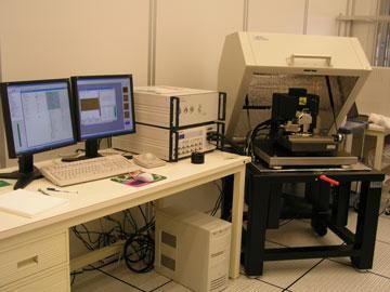
TappingMode AFM

Feedback Loop Electronics

TappingMode AFM operates by scanning a tip attached to the end of an oscillating
cantilever across the sample surface.
The cantilever is oscillated at or slightly below its resonance frequency with an
amplitude ranging typically from 20nm to 100nm. The tip lightly “taps” on the sample
surface during scanning, contacting the surface at the bottom of its swing.
The feedback loop maintains a constant oscillation amplitude by maintaining a constant
RMS of the oscillation signal acquired by the split photodiode detector.
The vertical position of the scanner at each (x,y) data point in order to maintain a
constant “setpoint” amplitude is stored by the computer to form the topographic image
of the sample surface. By maintaining a constant oscillation amplitude, a constant tip-
sample interaction is maintained during imaging.
Operation can take place in ambient and liquid environments. In liquid, the oscillation
need not be at the cantilever resonance.
When imaging in air, the typical amplitude of the oscillation allows the tip to contact the
surface through the adsorbed fluid layer without getting stuck.

TappingMode AFM

Advantages:
• Higher lateral resolution on most samples (1nm to 5nm).
• Lower forces and less damage to soft samples imaged in air.
• Lateral forces are virtually eliminated, so there is no scraping.
Disadvantages:

   Page | 2
• Slightly slower scan speed than contact mode AFM.

Abbreviated Instructions for the MultiMode AFM

Mode of Operation
In the Other Controls panel, set AFM Mode to Tapping, Contact, or choose the
appropriate profile and change the mode switch on the base to TMAFM or AFM & LFM
mode, respectively.

Mount Probe
1. Mount a probe into the cantilever holder. Be sure that it is in firm contact with the end
of the groove.
• Tapping: Use an etched single crystal silicon probe (TESP).
• Contact: Use a silicon nitride probe (NP).
2. Put the cantilever holder in the optical head. Secure the holder by tightening the
screw in the back of the optical head.

Select Scanner
Choose a scanner (A, E, or J). Mount and plug the scanner into the base. Attach the
corresponding springs to the microscope base. In the software, choose the appropriate
scanner parameters with Microscope > Select.

Mount Sample
Mount a sample on a metal disk with a “sticky-tab” (sample width should be limited to
the disk’s 15mm diameter). Mount the disk and sample on top of the scanner.

Place Optical Head on Scanner
1. Raise all three coarse-adjust screws on the scanner so that there is enough
clearance between the tip and sample when the optical head is placed on the scanner.
If using a JV or EV scanner, you only need to raise the motor screws.
2. Place the optical head on the scanner, still checking that the tip doesn’t touch the
sample. Attach the springs to the optical head.
3. Plug in the connector from the optical head to the base.
4. Bring the tip close to the sample keeping the head level by lowering all three coarse-
adjust screws.

Align Laser and Tip-Sample Approach (2 Methods)
1. Magnifier Method for Aligning Laser and Tip-Sample:
a. Focus on the side-view of the cantilever with the magnifier. If you are having trouble
finding the cantilever, try searching for the red light of the laser and focus on that. Use
the “paper method” described below for positioning the laser spot on the cantilever:
b. Move laser until it is at the front edge of the cantilever substrate. Move laser just off
the front edge and move laterally along the edge looking for the reflection of the laser
spot from the cantilever onto the paper. Center the laser on the cantilever at its end.

   Page | 3
c. Keeping the optical head level, focus on the laser reflection of the cantilever and
sample to bring the cantilever close to the sample. Use screws at the base of the optical
head (front and left) to position the cantilever over the area of interest on the sample.
2. Optical Viewing Microscope Method for Aligning Laser and Tip-Sample
a. Place the microscope on the optical microscope positioning stage.
b. Turn on the monitor and the light source.
c. Focus on the cantilever (zoom out, if using optical microscope equipped with zoom).

Use the base screws on the stage of the optical microscope to center the cantilever in
the field of view. Lower the focus of the optical microscope to the sample surface. You
will still see an out of focus “shadow” of the cantilever in the field of view. Keep the
optical head level while lowering the cantilever until it is almost in the same plane of
focus -keep the shadow of the cantilever in the field of view at all times. It is helpful to
go up and check the focus on the cantilever from time to time to see how close it is to
the sample surface.
d. Once the cantilever is close to the sample surface, adjust the laser so that it is
positioned over the cantilever. Use the two screws at the top of the optical head to move
the red laser spot onto the cantilever. You may need to change the field of view of the
optical microscope initially to find the laser spot.
e. Next use the “paper method” (as described under Magnifier Method) to fine position
the laser spot on the cantilever. Use the two screws at the base of the optical head
(front and left) to position the cantilever over the area of interest on the sample. As the
stepper motor moves during engagement, the cantilever will shift towards the back of
the microscope (unless you are using a Vertical Engage Scanner). This means that you
should place the cantilever in front of (below on the monitor) the area where you want to
engage.

Adjust Photodiode Signal
Note where the laser reflection enters the photodiode cavity. If necessary, adjust the
mirror (lever on back of optical head) to center the laser reflection into the photodiode
cavity. Leave the mirror at an angle such that the SUM signal (circular meter in bottom
LCD) is maximized.
• Tapping: Adjust the Vertical Difference value (bottom LCD) to zero using the screw
on the top left side of the optical head.
• Contact: Set the Contact AFM Output Signal value (Vertical Difference, top LCD) to -
2.0V using the screw on the top left side of the optical head. Adjust Horizontal
Difference value (bottom LCD) to zero using the screw on the back, left side of the
optical head.

Cantilever Tune (TappingMode Only)
Select View > Cantilever Tune (or select the Cantilever Tune icon). For Auto Tune
Controls, make sure Start Frequency is at 100 kHz and End Frequency is at 500 kHz.
Target Amplitude should be 2-3 volts. Click on Auto Tune. A “Tuning...” sign should

   Page | 4
appear and then disappear once Auto Tune is done. When finished, quit the Cantilever
Tune menu.

Set Initial Scan Parameters
In Scan Controls panel, set the initial Scan Size to 1 μm, X and Y Offsets to 0, and
Scan Angle to 0.
• Tapping: In the Feedback Controls panel, set Integral Gain to 0.4, Proportional
Gain to 0.6, and Scan Rate to 2 Hz.
• Contact: In the Feedback Controls panel, set the Setpoint is to 0 volts, the Integral
Gain to 2.0, the Proportional Gain to 3.0, and the Scan Rate to 2 Hz.

Engage
Select Motor > Engage (or select the Engage icon).

Adjust Scan Parameters
Tapping
a. Select View > Scope Mode (or click on the Scope Mode icon). Check to see if the
Trace and Retrace lines are tracking each other well (i.e. look similar). If they are
tracking, the lines should look the same, but they will not necessarily overlap each
other, either horizontally or vertically.

b. If they are tracking well, then your tip is scanning on the sample surface. You may
want to try keeping a minimum force between the tip and sample by clicking on
Setpoint and Realtime using the right arrow key to increase the Setpoint value
gradually, until the tip lifts off the surface and the Trace and Retrace lines no longer
track each other. Then decrease the Setpoint with the left arrow key until the Trace and
Retrace follow each other again. To make sure that the tip will continue to track the
surface, it is best to decrease the Setpoint one or two arrow clicks more with the left
arrow key. Then select
View > Image Mode (or click on the Image Mode icon) to view the image.
c. If they are not tracking well, adjust the Scan Rate, Gains and/or Setpoint to improve
the tracking. If Trace and Retrace look completely different, you may need to decrease
the Setpoint one or two clicks with the left arrow key until they start having common
features in both scan directions. Then, reduce Scan Rate to the lowest speed with
which you feel comfortable. For scan sizes of 1-3μm try scanning at 2Hz; for 5-10μm,
try 1Hz; and for large scans, try 1.0-0.5Hz. Next, try increasing the Integral Gain using
the right arrow key. As you increase the Integral Gain, increase the Proportional Gain
as well (Proportional Gain can usually be 30-100% more than Integral Gain). The
tracking should improve as the gains increase, although you will reach a value beyond
which the noise will increase as the feedback loop starts to oscillate. If this happens,
reduce the gains until the noise goes away. If Trace and Retrace still do not track
satisfactorily, the last thing to try is to reduce the Setpoint. Once the tip is tracking the
surface, select

   Page | 5
View > Image Mode (or click on the Image Mode icon) to view the image.

Set Desired Scan Size, Scan Angle, and Offsets
Once the scan parameters are optimized, scan size and other features may be adjusted
for capturing images for analysis. When changing the scan size value, keep in mind that
the scan rate will need to be lowered for larger scan sizes.

Realtime Operation
The Realtime parameters are located in the control panels which are available in the
Panels pull down menu. The main control panels for topographic imaging are “Scan
controls,” “Feedback Controls,” “Other Controls,” and “Channel 1.”
There are three primary feedback parameters that need adjusting every time you
engage the microscope to capture an image in TappingMode AFM or Contact Mode
AFM: Setpoint, Integral Gain, and Scan Rate.
To demonstrate how these parameters affect the image, examples of TappingMode
operation on the 10μm x 10μm pitch calibration grating will be shown. These examples
were acquired by viewing the Scope Mode (in the View menu), which displays a two-
dimensional view (X vs. Z) of the Trace (left-to-right) and Retrace (right-to-left) scan
lines being acquired in Realtime.
Scope Mode may be used to diagnose how well the tip is tracking the surface. If the
feedback parameters are adjusted optimally, the trace and retrace scan lines should
look very similar, but may not look completely identical.
An optimized scope trace of a 40μm TappingMode scan across the pits of the grating is
shown below.

                   Scope Trace with Optimized Realtime Parameters

Setpoint
The Setpoint parameter tells the feedback loop what amplitude (TappingMode) or
deflection (Contact Mode) to maintain during scanning.
Set this parameter so that the smallest amount of force is applied during scanning while
still maintaining a stable engagement on the surface.
If the setpoint is too close to the free air amplitude (TappingMode) or free air deflection
(Contact Mode) of the cantilever, the tip will not trace the topography properly.

   Page | 6
This problem will be more pronounced on downward slopes with respect to the scan
direction. An example of this is shown below.
Scope Trace Demonstrating the Effect of the Setpoint Being Adjusted Too Close to the
Free Air Amplitude During TappingMode AFM
Notice that the tip tracks the surface up the sidewall properly but not down the sidewall
with respect to the scan direction. This occurs on opposite sides of features for the
Trace and Retrace scan directions.
This problem can be remedied by decreasing the Setpoint in TappingMode, or
increasing the Setpoint in Contact Mode.
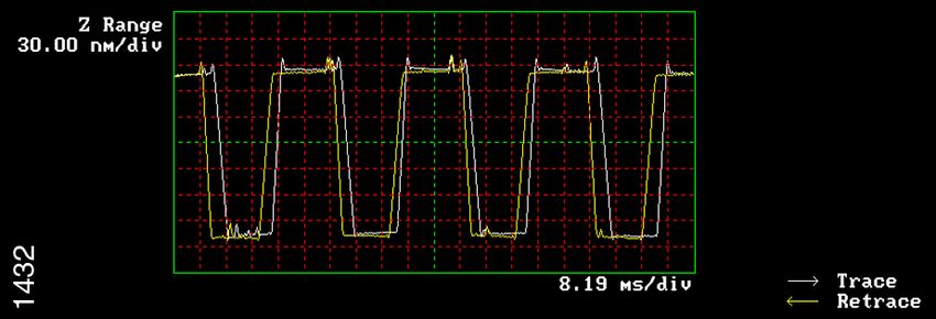
Integral Gain
The Integral Gain controls the amount of the integrated error signal used in the
feedback calculation. The higher this parameter is set, the better the tip will track the
sample topography.
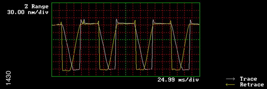
However, if the integral gain is set too high, noise due to feedback oscillation will be
introduced into the scan, as shown below.
Scope Trace Demonstrating the High Frequency Noise that Occurs when the Integral
Gain is Set Too High
Page | 7Setting the integral gain too low may result in the tip not tracking the surface properly,
as shown below.
Scope Trace Demonstrating the Effect of Setting the Integral Gain Too Low
Set the Integral Gain as high as possible by increasing the gain until noise is seen, then
reduce the gain just lower than the value where the noise disappears.
Scan Rate
The Scan Rate is the number of trace and retrace scan lines performed per second
(Hz).
• For example, with a scan rate set to 1Hz, the tip will scan forward and back (trace and
retrace) in 1 second. Set this value so that the feedback loop has time to respond to
changes in the sample topography. Setting the scan rate too high will result in poor
tracking of the surface, as shown below.
Scope Trace Demonstrating the Effect of Setting the Scan Rate Too High
The actual tip speed or of the tip depends on two parameters: Scan Rate and Scan
Size. Since the Scan Rate units are lines per second (Hz), increasing the Scan Size
without changing the Scan Rate actually increases the scan velocity of the tip.
• For example, if the Scan Rate is 1Hz and the Scan Size is 1μm, the scan velocity is
2μm/sec (since it performs the trace and retrace scans in 1 sec). By increasing the Scan
Size to 100μm, the scan velocity increases to 200μm/sec if the Scan Rate remains 1Hz.
The Scan Rate setting will greatly depend on the scan size and the height of the
features being imaged. In general, the taller the features and/or the larger the scan size,
the slower the scan rate. Typical Scan Rate settings are 0.5 to 2.0Hz for TappingMode
and 1 to 4Hz for Contact Mode.
Page | 8Other Important Parameters Scan Size: Adjusts the size of the X,Y scan area X Offset, Y Offset: Translates the scan area in X and Y directions without changing scan size Note: The Zoom and Offset commands found on the display monitor may also be used to change the scan size and X and Y offsets. Scan Angle: Controls the angle of the fast scan direction of the scanner with respect to the X axis Samples/line: Determines the number of data points or pixels in X and Y (128, 256, or 512) Slow Scan Axis: Enables and Disables movement of the scanner in the direction of the slow scan axis. (Y direction at 0° Scan Angle) Proportional Gain: Controls the amount of proportional error signal used in feedback calculation Typically set 30 to 100% higher than the Integral Gain Data Type: Selects the signal viewed on the display monitor - this parameter is set to Height for topographical measurements Line Direction: Selects the direction of the fast scan during data collection: Trace (left to right) or Retrace (right to left). Microscope Mode: Sets mode of operation to Tapping, Contact, or Force Mod Data Scale: Controls the vertical scale of the full height of the display and color bar. This parameter does not effect the Realtime operation of the microscope, only the expansion and contraction of the color scale. Z-limit: Allows the 16 bits of the digital-to-analog converters to be applied to a smaller vertical range. This has the effect of increasing the vertical sampling resolution and should be used for imaging very smooth surfaces (
• Offset: Saves the image without removing the tilt with a first order planefit, but does
remove the Z offset.
• None: Saves the image without removing the tilt or the Z offset.

The Full setting is commonly used for everyday imaging. However, the Offset setting
can be useful when a first order planefit would negatively affect the measurement of
interest. This can be demonstrated in the example below. If the measurement of interest
is the height of the step, then setting the Offline Planefit to Full will result in the tilting of
the data. However, if the Offline Planefit is set to Offset, then a planefit is not applied
and the step orientation is not altered. If the Full setting were applied, a first order
planefit could be applied in the Offline software to reoriented the features without
negatively affecting the measurement.

Once images are captured during Realtime operation, they are viewed and measured
with the Offline commands. Here we will touch on a few of the basic operations and
functions.
• Each captured image is immediately stored in the Capture directory in Offline.
• Access to different disk drives is available at the top of the file directory panel. The !:\
drive is the Capture directory, the A:\ drive is a floppy drive, the C:\, D:\ and E:\ are
usually the computer hard drives. If the system has additional drives, they are set
through Z:\.
• The data management commands are found in the File pull down menu. This menu
contains the Move, Copy, Delete, Rename, and Create Directory commands for
transferring data between directories.
• The Browse command, also under the File menu, places up to twenty-four images on
the screen with a variety of commands available at the top of the Browse screen. There
is also a File menu within the Browse commands which provides the ability to specify in
any order which images to Move, Copy, Delete, or Rename. Browse also provides the
ability to view two images side-by-side by using Dual, or to view up to six images side-
by-side using Multi.

Image Analysis
A wide variety of analysis functions are available in the Analyze menu in the Offline for
measuring captured SPM images.
Each of the analysis routines is useful and described in detail in the Command
Reference Manual.
Some of the most commonly used analysis routines are briefly described below.

Section
Depth, height, width, and angular measurements can be easily made with Section. For
an example,
see the following figure.

   Page | 10
Cross-Sectional Measurement on a DVD Replica Disk

A cross-sectional line can be drawn across any part of the image, and the vertical profile
along that line is displayed. The Cursor menu located at the top of the Display monitor
provides the ability to draw a fixed, moving, or averaged cross section.
Up to three pairs of cursors may be placed on the line section at any point to make
horizontal, vertical, and angular measurements. These measurements are reported in
the box at the lower right of the screen. Cursors may be added or deleted with the
Marker menu located at the top of the Display monitor. The measurements are
displayed in the same colors as the corresponding markers. The power spectrum (fast
Fourier transform (FFT)) along the cross section is displayed in the lower center
window. The cursor may be used to determine the predominate periodicities along the
cross section by placing it at peaks in the spectrum. The roughness measurements of
the portion of the cross section between the two colored cursors are displayed in the
window in the upper right.

Roughness
Roughness measurements can be performed over an entire image or a selected portion
of the image with Roughness.

     Roughness Measurements on Epitaxial SiGe Image Showing Growth Defects

   Page | 11
There are a wide variety of measurements made in Roughness. The roughness parameters which are displayed are chosen under the Screen Layout menu. The measurements made on the entire image are displayed under “Image Statistics.” Roughness measurements of a specific area may be determined by using the cursor to draw a box on the image. After selecting “Execute,” the measurements within the selected area are displayed under “Box Statistics.” The most common measurements are the following: 1. RMS (Rq): The Root Mean Square (RMS) Roughness is the standard deviation of the Z values within a given area. • Zave is the average Z value within the given area, Zi is the current Z value, and N is the number of points within a given area. • Ra: The Mean Roughness (Ra) represents the arithmetic average of the deviations from the center plane. • Zcp is the Z value of the center plane, and Zi is the current Z value, and N is the number of points within a given area. Note: The above equations for RMS and Ra are presented for ease in understanding. 2. Rmax: The difference in height between the highest and lowest points on the surface relative to the Mean Plane 3. Surface Area: The three-dimensional area of a given region. This value is the sum of the area of all of the triangles formed by three adjacent data points. 4. Surface Area diff: The percentage increase of the three dimensional surface area over the two dimensional surface area. Bearing Bearing ratio determination and depth histogram measurements are possible with Bearing. Bearing provides a method to analyze how much of the surface lies below or above a given height. Page | 12
The “bearing ratio” of the surface is the percentage of the surface at a specific depth
with respect to the entire area analyzed. (See manual for further description)
The depth histogram plots depth versus percentage of occurrence of data at different
depths.
By enabling the Histogram Cursor (top menu, display screen), two cursors are available
on the histogram to make relative depth measurements.
Area depth measurements can be made by placing the two cursors at peaks
representing different feature heights. The area depth measurement can be made by
determining the relative depth between the two cursors.
• Planefit and/or Flatten may need to be performed before making this measurement.
This will produce sharper peaks in the depth histogram. The Depth feature may be
used to make automated depth histogram measurements over many images. (See
manual for details)

         Area Depth Measurement of GaAs Lines using the Bearing Histogram

Filters
There are a wide range of modification functions found in the Modify menu that may be
applied to an image once it has been captured. These functions are explained in detail
in the Command Reference Manual.
It should be kept in mind that by using any modification functions, the data is being
changed which may or may not affect the measurements of interest. In general, it is
good practice to modify the image as little as possible, and to understand how the
applied function will affect the image and measurements.

   Page | 13
Flatten may be used to remove image artifacts due to vertical (Z) scanner drift, image
bow, skips, and anything else that may have resulted in a vertical offset between scan
lines.
Flattening modifies the image on a line-by-line basis. It consists of removing the
vertical offset between scan lines in the fast scan direction (X at 0° scan angle) by
calculating a least-squares fit polynomial for a scan line, and subtracting the polynomial
fit from the original scan line.
• This has the affect of making the average Z value of each scan line equal to 0V out of
the +/- 220V z-range. Flattening can be performed by applying a 0th, 1st, 2nd, or 3rd
order polynomial fit to each scan line.
Typical Image Artifacts
If the tip becomes worn or if debris attaches itself to the end of the tip, the features in
the image may all have the same shape. What is really being imaged is the worn shape
of the tip or the shape of the debris, not the morphology of the surface features.
Dull or Dirty Tip
Double or multiple tip images are formed with a tip with two or more end points which
contact the
sample while imaging. The above images are examples.
Page | 14Double or Multiple Tips
Loose debris on the sample surface can cause loss of image resolution and can
produce streaking in the image. The image on the left is an example of the loss of
resolution due to the build up of contamination on the tip when scanning from bottom-to-
top. It can be seen how the small elongated features become represented as larger,
rounded features until the debris detaches from the tip near the top of the scan. The
image on the right is an example of skips and streaking caused by loose debris on the
sample surface.
Often, loose debris can be swept out of the image area after a few scans, making it
possible to acquire a relatively clean image. Skips can also be removed from a captured
image with the Erase Scan Lines function.
Contamination from Sample Surface
Page | 15Interference between the incident and reflected light from the sample surface can
produce a sinusoidal pattern on the image with a period typically ranging between 1.5-
2.5μm. This artifact is most often seen in contact mode on highly reflective surfaces in
force calibration plots and occasionally in TappingMode images. This artifact can
usually be reduced or eliminated by adjusting the laser alignment so that more light
reflects off the back of the cantilever and less light reflects off the sample surface, or by
using a cantilever with a more reflective coating (MESP, TESPA).
Optical Interference
When the feedback parameters are not adjusted properly, the tip will not trace down the
back side of the features in TappingMode. An example of this can be seen in the image
on the left which as scanned from left-to-right (trace) producing “tails” on the colloidal
gold spheres. The image on the right is the same area imaged with a lower setpoint
voltage, increased gains, and slower scan rate.
Page | 16In TappingMode, when operating on the high frequency side of the resonance peak,
rings may appear around raised features which may make them appear as if they are
“surrounded by water.” An example of this can be seen in the image of the Ti grains on
the left. Decreasing the Drive Frequency during imaging can eliminate this artifact, as
shown in the image on the right (when reducing the Drive Frequency, the Setpoint
voltage may need to be reduced as well).
Rings During High Frequency Operation
The arch shaped bow in the scanner becomes visible at large scan sizes (left). The bow
in this image can be removed by performing a 2nd order Planefit in X and Y (right).
(Data Scale = 30nm)
Page | 172nd Order Bow
At large scan sizes, the bow in the scanner may take on an S-shaped appearance (left).
This may be removed by performing a 3rd order planefit in X and Y (right). (Data Scale
= 324nm).
3rd Order Bow
Page | 18You can also read